Precise excitation-inhibition balance controls gain and timing in the hippocampus
- Tata Institute of Fundamental Research, India
Figures
Figure 1 with 1 supplement
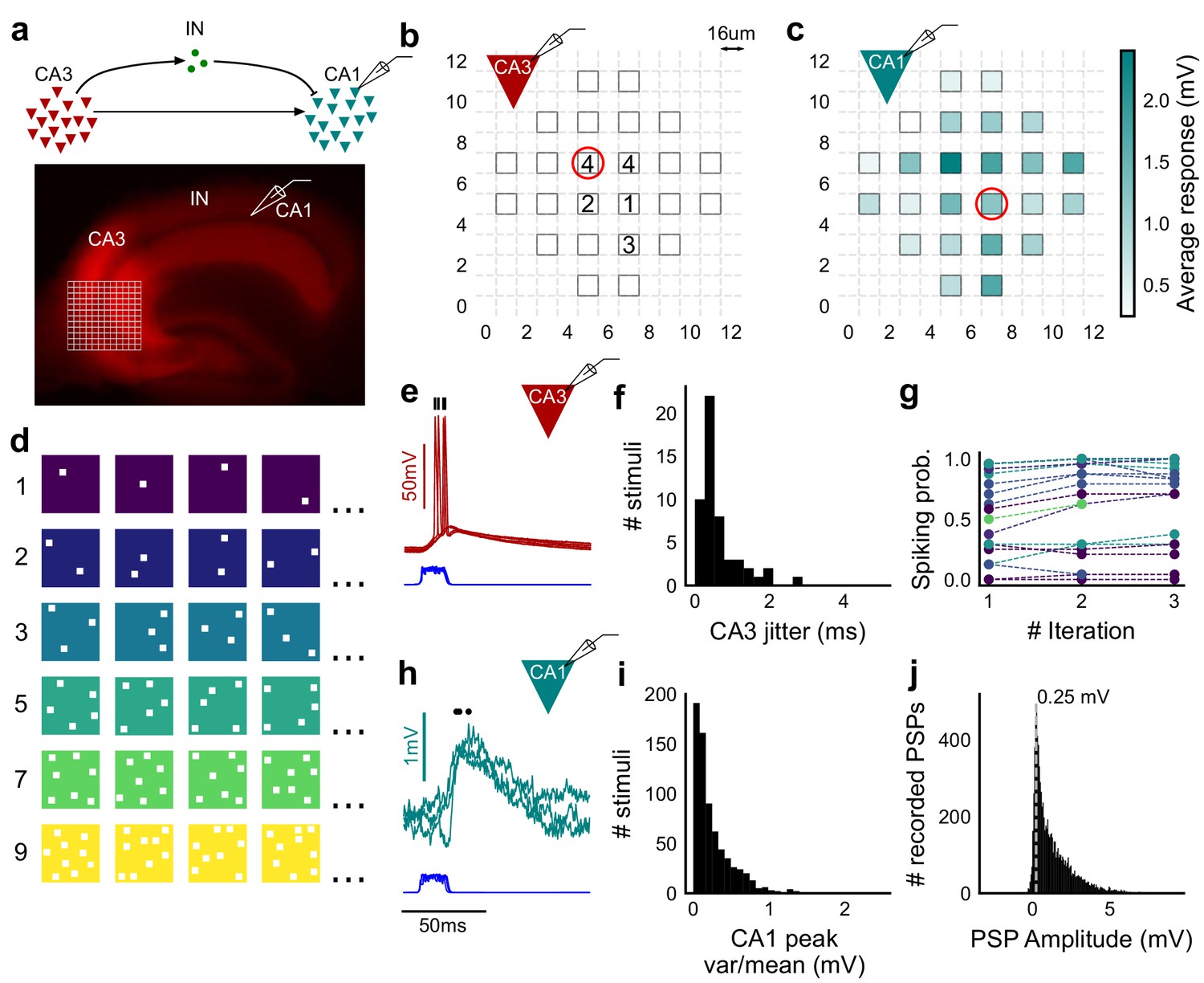
Stimulating CA3-CA1 network with hundreds of optical patterns.
(a) Top, schematic of the CA3-CA1 circuit with direct excitation and feedforward inhibition. Bottom, image of a hippocampus slice expressing ChR2-tdTomato (red) in CA3 in a Cre-dependent manner. Optical stimulation grid (not drawn to scale) was centered at the CA3 cell body layer and CA1 neurons were patched. (b) Spike response map of CA3 neuron responses with one grid square active at a time. A CA3 neuron was patched and optically stimulated, in random spatio-temporal order, on the grid locations marked with grey border. This cell spiked (marked with number inside representing spike counts over four trials) in 5 out of 24 such one square stimuli delivered. (c) Heatmap of CA1 responses while CA3 neurons were stimulated with one square optical stimuli. Colormap represents peak Vm change averaged over three repeats. (d) Schematic of optical stimulus patterns. Examples of combinations of N-square stimuli where N could be 1, 2, 3, 5, 7 or 9 (in rows). (e) Spikes in response to four repeats for the circled square, in b. Spike times are marked with a black tick, showing variability in evoked peak times. Blue trace at the bottom represents photodiode measurement of the stimulus duration. Scale bar for time, same as h. (f) Distribution of jitter in spike timing (SD) for all stimuli for all CA3 cells (n = 8 cells). (g) CA3 spiking probability (fraction of times a neuron spiked across 24 stimuli, repeated thrice) is consistent over a single recording session. Randomization of the stimulus pattern prevented ChR2 desensitization. Circles, colored as in d depict spiking probability on each repeat of a stimulus set with connecting lines tracking three repeats of the set (n = 7 cells). (h) PSPs in response to three repeats of the circled square in c. Peak times are marked with an asterisk. Blue traces at the bottom represent corresponding photodiode traces for the stimulus duration. (i) Distribution of peak PSP amplitude variability (variance/mean) for all 1-square responses (n = 28 cells, stimuli = 695). (j) Histogram of peak amplitudes of all PSPs elicited by all 1-square stimuli, over all CA1 cells. Grey dotted line marks the mode (n = 38 cells, trials = 8845).
Figure 1—figure supplement 1
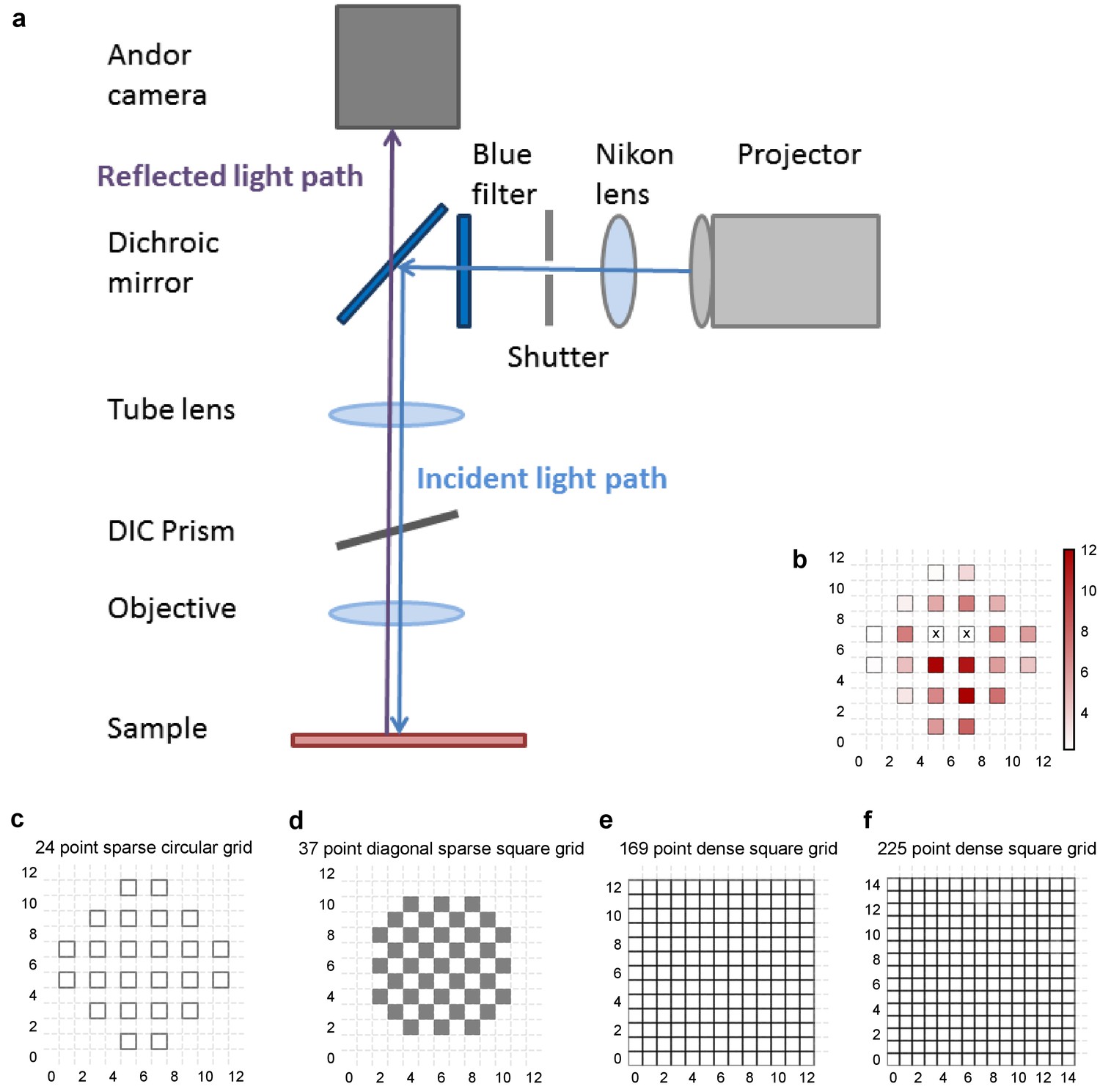
Experiment design.
(a) Schematic of the light path of patterned optical stimulation. Projector’s output was minified using a lens and introduced into the light path of the microscope by reflecting off of a dichroic. We could thus focus arbitrary minified patterns at the sample plane, and switch them at short intervals. (b) Heat map of CA3 neuron responses with one grid square active at a time, from the neuron in Figure 1b. Color in grid squares represents peak Vm change from baseline, averaged over trials when the neuron did not spike. Locations where the cell spiked all four times are marked with a cross. (c–f) Four different kinds of grids used for photostimulation. The grid was made sparser to avoid stimulation of the same region with light from nearby photostimulation squares. The four different grids were (from left to right): 24 square circular sparse grid (Figure 1) (13 cells), 37 point sparse circular grid (6 cells), 13 × 13 dense grid (9 cells), 15 × 15 dense grid (10 cells). For one cell we used a fifth kind of grid: 112 point dense circular grid (not shown in figure).
Figure 2 with 2 supplements

Excitation and inhibition are tightly balanced for all stimuli to a CA1 cell.
(a) Monosynaptic excitatory postsynaptic currents (EPSCs, at −70 mV) and disynaptic inhibitory postsynaptic currents (IPSCs, at 0 mV) in response to five different stimulus combinations of 5 squares each. All combinations show proportional excitatory and inhibitory currents over six repeats. Top, schematic of 5-square stimuli. (b) EPSCs and IPSCs are elicited with the same I/E ratio in response to six repeats of a combination, and across six different stimuli from 1 square to nine squares, for the same cell as in a. Top, schematic of the stimuli. (c) Area under the curve for EPSC and IPSC responses, obtained by averaging over six repeats, plotted against each other for all stimuli to the cell in a, b. Error bars are s.d. (d) Summary of I/E ratios for all cells (n = 13 cells). (e) Summary for all cells of R2 values of linear regression fits through all points. Note that 11 out of 13 cells had R2 greater than 0.9, implying strong proportionality. (f) Same as e, but with linear regression fits for 1 and 2 square responses, showing that even small number of synapses are balanced for excitation and inhibition (n = 9 cells). (g) Phase plot from the model showing how tuning of synapses (ρ) affects observation of EI balance (R2) for various values of variance/mean of the basal weight distribution. Changing the scale of the basal synaptic weight distributions against tuning parameter ρ affects goodness of EI balance fits. Arrow indicates where our observed synaptic weight distribution lay. (h) Example of EI correlations (from data) for 1 and 2 square inputs for an example cell. Bottom, schematic of the stimuli. Excitation and inhibition are colored olive and purple, respectively. Error bars are s.d. (i) Examples of EI correlation (from model) for small number of synapses, from the row marked with arrow in g. The left and right curves show low and high correlations in mean amplitude when EI synapses are untuned (ρ = 0) and tuned respectively (ρ = 1) (A.U. = Arbitrary Units). Colors, same as h. Error bars are s.d.
Figure 2—figure supplement 1
Detailed balance in CA3-CA1 feedforward network.
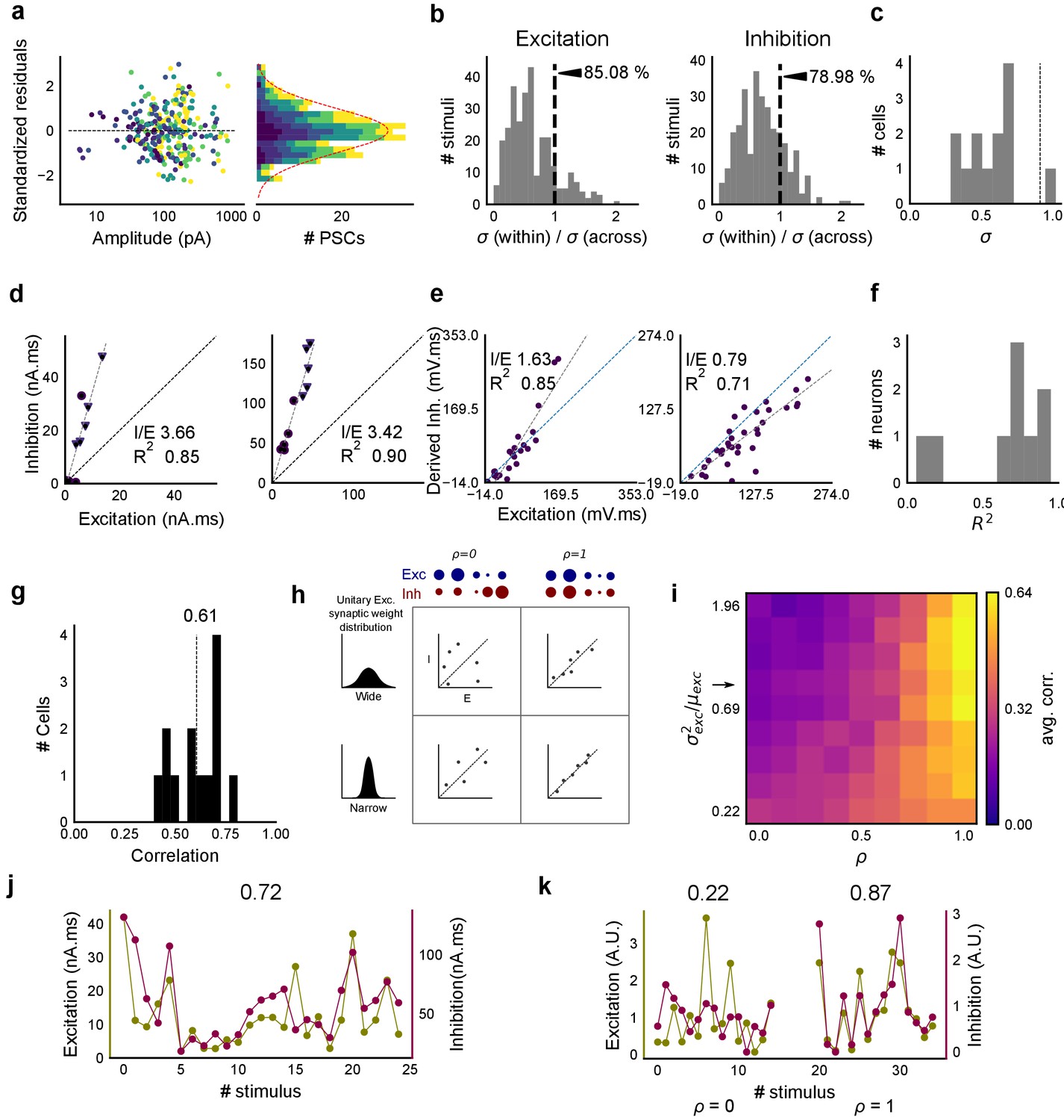
(a) Plot of residuals for all inputs (colored by N-square as shown in Figure 1d) of all cells, normalized by their standard deviation. The residuals were calculated by subtracting the actual values of inhibition from the values predicted by the regression line across the Excitation-Inhibition plot. These were then standardised by dividing individual residual values by the standard deviation across all stimuli of the same number of squares. We found that standardized residuals for different input squares were distributed symmetrically across 0, showing that the I/E ratios did not change substantially across the cell. Variability within stimulus repeats compared with that across all stimuli grouped by the number of squares, for excitation (left) and inhibition (right). For both, within stimulus variability is lower. (b) Variability over repeats of a stimulus (within) divided by variability across all stimuli of the same number of squares delivered to a cell (across), for excitation (left) and inhibition (right). Dotted line represents equal within and across variability. For both excitation and inhibition, within-stimulus variability is lower (n = 13 cells). (c) Standard deviation of I/E ratios across stimuli for a given cell was lower than that across all cells (dotted line) for 12 out of 13 cells. (d) Two example cells where EI balance can be observed for 1 and 2 square data from voltage clamped cells (Summary plot in Figure 2f). (e) Two example cells where EI balance can be observed for one square data from current clamped cells, as shown in Figure 5d. (f) Summary of R2 for one square data from all current clamped cells (n = 9). (g) Histogram of correlation between standard deviations (s.d.) for excitation and inhibition for all stimuli over individual cells. Mean correlation = 0.61 (n = 13 cells). (h) A schematic for the detailed balance model. EI correlations increase with increase in ρ, as well as with decrease in variance of the distribution of basal excitatory synaptic weights. (i) Phase plot, similar to Figure 2g, but with correlations of standard deviations for excitation and inhibition. Arrow marks the row with our estimated synaptic weight distribution width. (j) Example cell with 0.72 correlation between s.d. of excitation and inhibition repeats over individual stimuli. Excitation and inhibition are colored olive and purple respectively. (k) Examples for s.d. correlation from the row marked with arrow, for untuned (left, ρ = 0, corr = 0.22) and tuned (right, ρ = 1, corr = 0.87) synapses (A.U. = Arbitrary Units). Colors, same as i. Error bars are s.d.
Figure 2—figure supplement 2
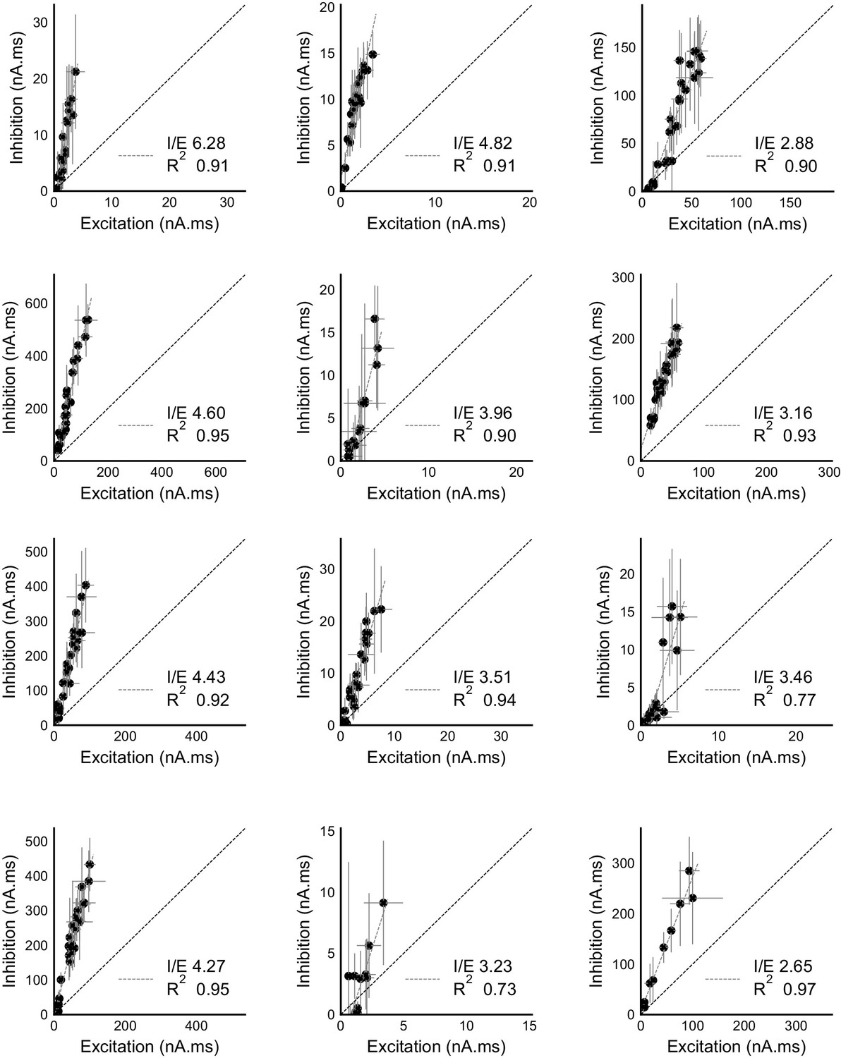
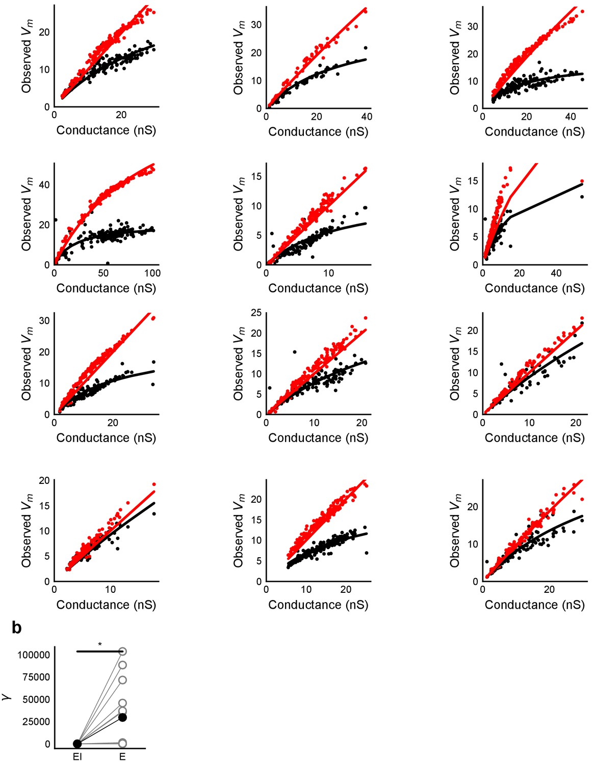
Raw data from all cells showing precise balance between excitation and inhibition.
Individual plots for area under the curve for excitation and inhibition recorded from all cells (except the display cell in Figure 2c). These were measured by clamping the cells at inhibitory (−70 mV) and excitatory (0 mV) reversal potentials respectively. Cells exhibit close proportionality between excitation and inhibition. The I/E ratio (slope) and the R2 (goodness of fit) for each cell are mentioned in their individual plots. Error bars are s.d.
Figure 3 with 1 supplement
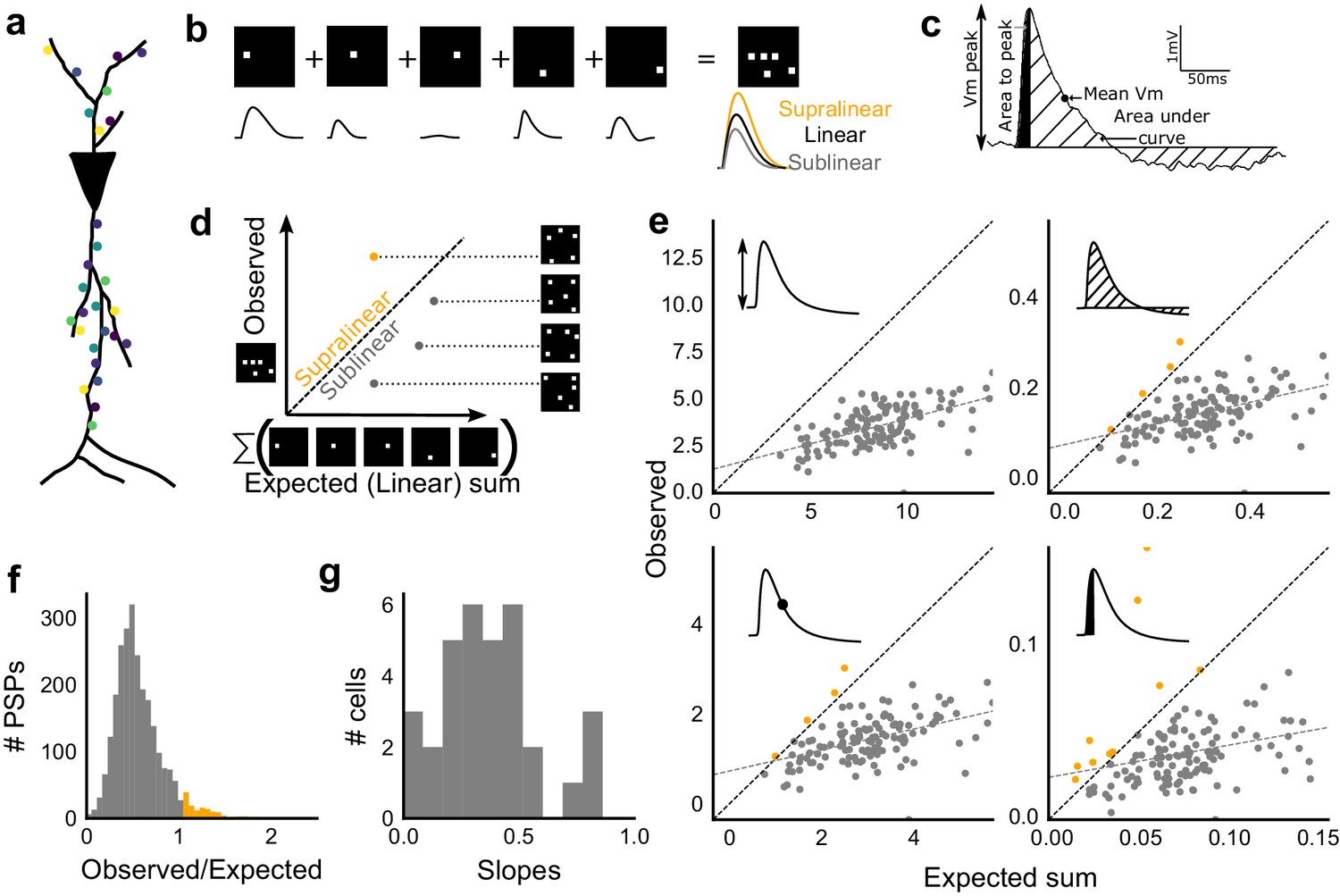
Excitatory and feed-forward inhibitory inputs from CA3 integrate sublinearly at CA1.
(a) Schematic of a neuron receiving synaptic input distributed over its dendritic tree. (b) Schematic of input integration. Top, five 1-square stimuli presented individually, and a single 5-square stimulus comprising of the same squares. Bottom, PSPs elicited as a response to these stimuli. 5-square PSP can be larger (supralinear, orange), equal to (linear, black), or smaller (sublinear, grey) than the sum of the single square PSPs. (c) A PSP trace marked with the four measures used for further calculations. PSP peak, PSP area, area to peak and mean voltage are indicated. (d) Schematic of the input integration plot. Each circle represents response to one stimulus combination. ‘Observed’ (true response of 5 square stimulation) on Y-axis and ‘Expected’ (linear sum of 1 square responses) is on X-axis. (e) Most responses for a given cell show sublinear summation for a 5-square stimulus. The four panels show sublinear responses for four different measures (mentioned in c) for the same cell. The grey dotted line is the regression line and the slope of the line is the scaling factor for the responses for that cell. For peak (mV), area (mV.ms), average (mV), and area to peak (mV.ms); slope = 0.27, 0.23, 0.23, 0.18; R2 0.57, 0.46, 0.46, 0.26, respectively. The responses to AUC and average are similar because of the similarity in the nature of the measure. (f) Distribution of Observed/Expected ratio of peaks of all responses for all 5-square stimuli (mean = 0.57, s.d. = 0.31), from all recorded cells pooled. 93.35% responses to 5-square stimuli were sublinear (2513 PSPs, n = 33 cells). (g) Distribution of slopes for peak amplitude of 5-square stimuli (mean = 0.38, s.d. = 0.22). Regression lines for all cells show that all cells display sublinear (<1 slope) summation (n = 33 cells).
Figure 3—figure supplement 1

Summation at CA3-CA1 network is sublinear.
(a) Responses to 1-square photostimulation at CA3 were similar in both Control and GABAzine conditions, except close to the tail of the distribution (n = 11, Control: 1092 trials, GABAzine: 1173 trials). This demonstrates that there is very little inhibitory effect on peak Vm with one square photostimulation. (b) Responses to 9-squares photostimulation lead to much larger responses in the presence of GABAzine than in its absence (n = 3, Control: 142 trials, GABAzine: 144 trials). Compare this with a. (c) Slope values for three other measures (area under curve, mean voltage and area to peak) of the observed PSP on five square stimulation in all cells. Sublinearity is seen in all four measures (n = 33 cells). The slope for first measure, peak Vm, is displayed in Figure 3g. Area under curve and Mean voltage panels look alike due to the similarity in the nature of the measure. (d) Summation plots analogous to those in Figure 3f for the remaining 2, 3, 7 and 9 stimuli. Observed/Expected (O/E) ratio for most stimuli was less than 1, showing sublinear summation (grey).
Figure 4 with 2 supplements
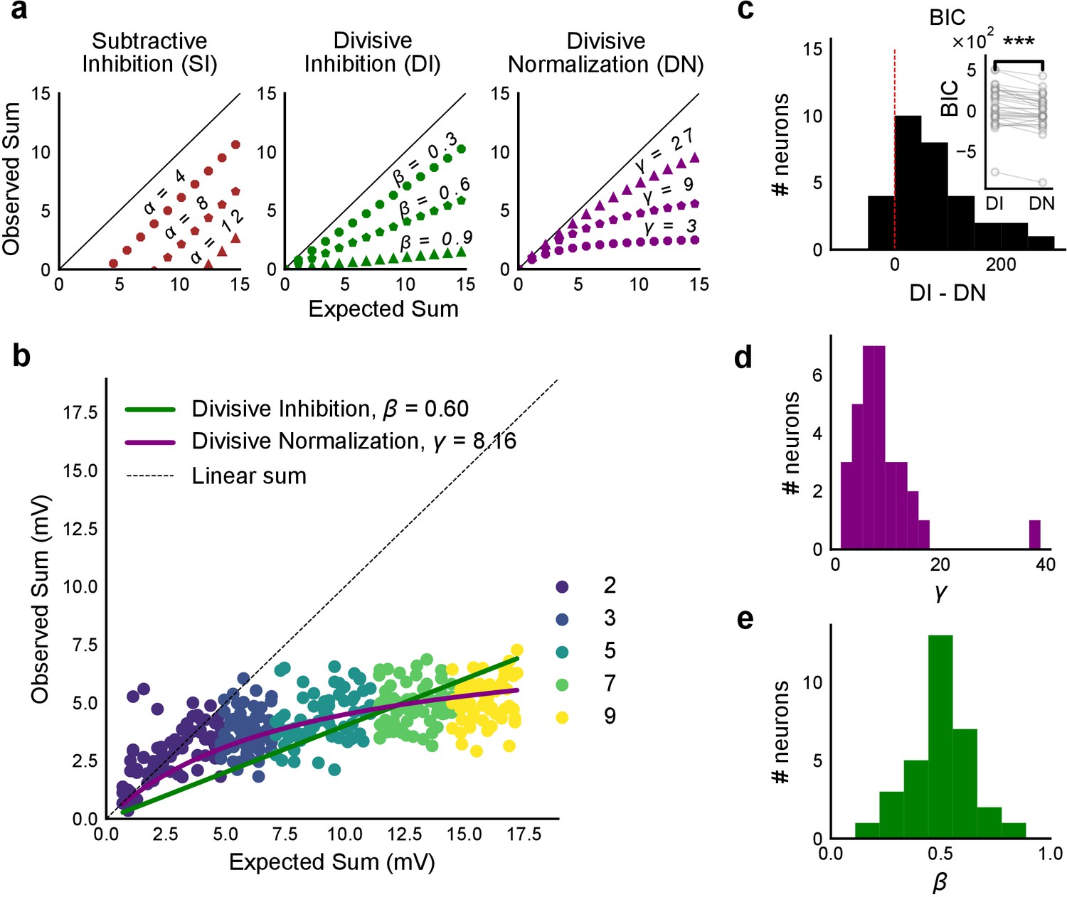
Over a wide input range, integration of CA3 excitatory and feed-forward inhibitory input leads to SDN at CA1.
(a) Three phenomenological models of how inhibition interacts with excitation and modulates membrane potential: (left to right) Subtractive Inhibition (SI), Divisive Inhibition (DI) and Divisive Normalization (DN). Note how parameters α, β and γ from Equation (1) affect response output. (b) Divisive normalization seen in a cell stimulated with 2, 3, 5, 7 and 9 square combinations. DN and DI model fits are shown in purple and green, respectively. (c) Difference in Bayesian Information Criterion (BIC) values for the two models - DI and DN. Most differences between BIC for DI and DN were less than 0, which implied that DN model fit better, accounting for the number of variables used. Insets show raw BIC values. Raw BIC values were consistently lower for DN model, indicating better fit (Two-tailed paired t-test, p<0.00005, n = 32 cells). (d) Distribution of the parameter γ of the DN fit for all cells (median = 7.9, n = 32 cells). Compare with a, b to observe the extent of normalization. (e) Distribution of the parameter beta of the DI fit for all cells (mean = 0.5, n = 32 cells). Values are less than 1, indicating sublinear behaviour.
Figure 4—figure supplement 1
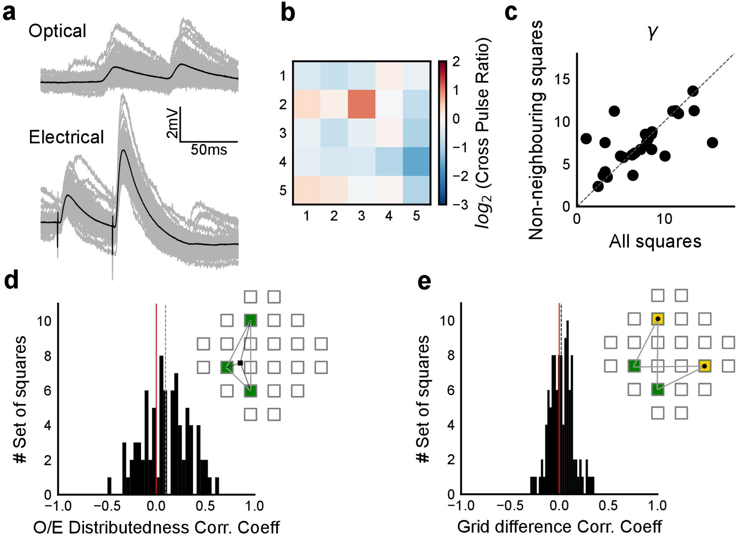
Interaction of squares does not affect summation unidirectionally.
(a) Example cell showing PPF with electrical, but not with optical stimulation. Individual traces are in grey and black is the average trace. (b) Cross Pulse Ratio (Materials and methods) of 25 pairs of stimuli (from five photostimulation squares) presented to an example cell, different from that in a. Ratio less than one for self-self pairs, on the diagonal, implies lack of facilitation. (c) We restricted our analysis to non-bordering squares and fit the subthreshold divisive normalization model and checked for the value of the normalization parameter (γ). The degree of sublinearity and the input-output curve remained unchanged, as indicated by the similarity in the values of DN parameter γ, ruling out the hypothesis that interactions between neighboring squares account for the observed sublinearity in the SDN curve. (d) Median correlation (0.09) between distributedness of the photostimulation squares and the O/E ratio shows that distances between grid squares do not have a unidirectional relationship with the extent of sublinearity. (e) Median correlation (0.02) between how close the patterns were on the grid to the measured voltage response of CA1 again shows no unidirectional effect of physical proximity of patterns.
Figure 4—figure supplement 2
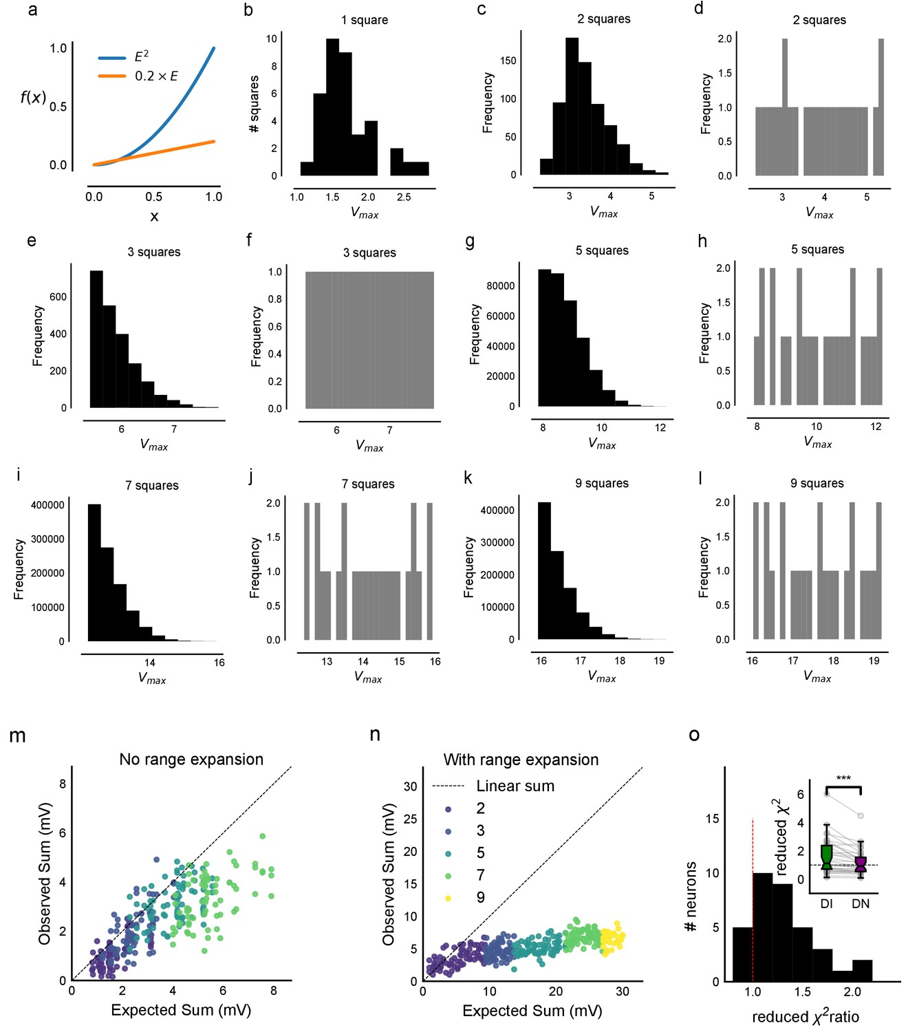
Input range expansion for observing nonlinear summation and divisive normalization.
(a) A large range of stimulus strengths is required to detect nonlinearity in summation and to characterize divisive normalization. Comparing a nonlinear function of x, f(x) = x2 (blue) with a linear function f(x)=0.2 x (orange). It is difficult to distinguish between the two possibilities (from x = 0. to x = 0.2). However, across a larger range of x, differences can be seen. (b–l) In order to sample uniformly and over a wider input range of a cell (x axis, labelled Expected sum), we did ‘range expansion’ for some cells (n = 6 cells) as follows. A 37-point grid (Figure 1—figure supplement 1c) was used for these experiments. For a given cell, we first measured the 1-square responses to all 37 grid squares. Then, the 1-square responses were binned into 24 bins, and one member was picked from each bin randomly. In case there were fewer than than one member per bin, other bins were resampled without replacement until the total number was 24. Using this, we generated the distributions of expected sum of N-squares (N = 2, 3, 5, 7, 9). The distributions of the next N-square was truncated such that its minimum began at the maximum of the last N-square distribution (distributions in black, first column of all rows). For example, if the set of squares were 2, 3, 5, 7, 9, we picked the squares such that the distribution of 5 squares started from the end of 3 squares. We then sampled uniformly from this reduced distribution (distributions in grey, second column of all rows). This allowed us to uniformly sample from the entire theoretically possible range, and hence ensure that we observed summation over a wide range of inputs (as explained in a). (m, n) Responses from one cell without (m) and one with (n) range expansion are shown. Note that responses from different N-squares (shown in different colors, marked as in Figure 1d), are overlapping in the Expected-axis for m, while the process of range expansion enforces exploration of a large input range in a non-overlapping manner in n. (o) Reduced chi-square fits confirm DN model fits better than DI. In addition to BIC (Figure 4c), we used the reduced chi-square fit test to compare the two models of inhibitory computations (divisive inhibition (DI) and divisive normalization (DN)). Divisive normalization model (Equation 3) almost always fit better than divisive inhibition model (Equation 2) for reduced chi-square, as it did for BIC (Figure 4b and c). This figure shows the reduced chi-square ratio plotted for DI and DN models (DI/DN). Values close to one imply good fits, while lesser and greater than one imply over and under-fitting the data respectively. Again, DN is on average closer to one (inset), and the reduced chi-square ratio is almost always larger than one, implying that DN model fit is better than a DI model fit (n = 32 cells).
Figure 5
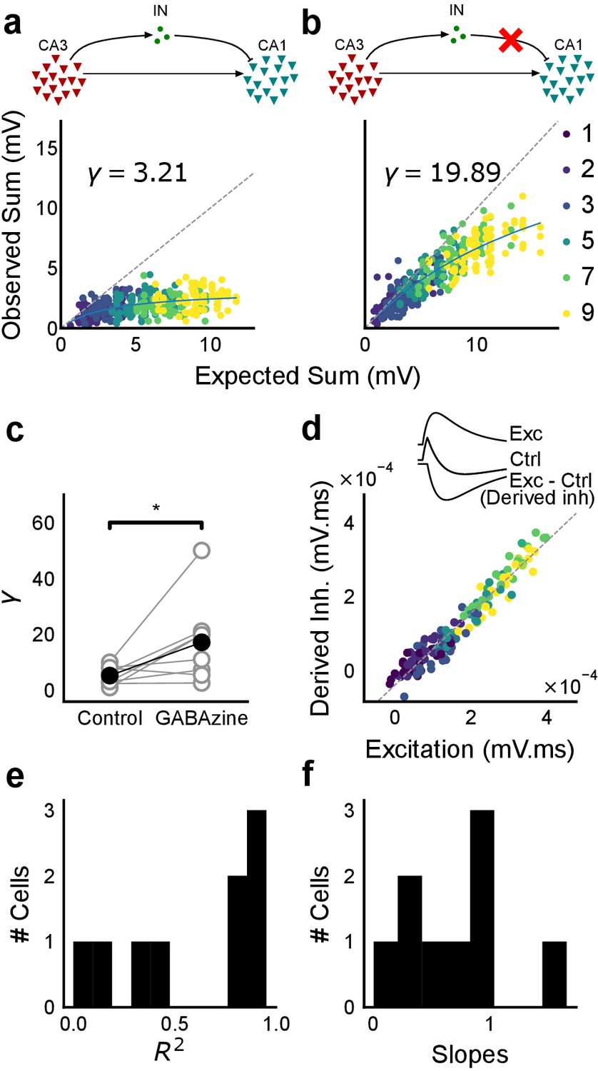
Blocking balanced inhibition at resting membrane potential attenuates SDN.
(a) Top, schematic of experiment condition. Bottom, a cell showing divisive normalization in control condition. (b) Top, schematic of experiment condition with feedforward inhibition blocked (2 uM GABAzine). Bottom, responses of the same cell with inhibition blocked. The responses are much closer to the linear summation line (dashed). The blue lines in a, b are the fits of the DN model. The value of γ of the fit increases when inhibition is blocked. (c) Parameter γ was larger with GABAzine in bath (Wilcoxon rank sum test, p<0.05, n = 8 cells), implying reduction in normalization with inhibition blocked. (d) Excitation versus derived inhibition for all points for the cell shown in a (area under the curve) (Slope = 0.97, r-square = 0.93, x-intercept = 3.75e-5 mV.ms). Proportionality was seen for all responses at resting membrane potential. Top, ‘Derived inhibition’ was calculated by subtracting control PSP from the excitatory (GABAzine) PSP for each stimulus combination. (e,f) R2 (median = 0.8) and slope values (median = 0.7) for all cells (n = 8 cells), showing tight IPSP/EPSP proportionality, and slightly more excitation than inhibition at resting membrane potentials.
Figure 6 with 2 supplements

Conductance model predicts Excitatory-Inhibitory delay as an important parameter for divisive normalization.
(a) Subthreshold responses from HH model, simulated with traces recorded from one voltage clamped cell (Figure 2). Non-linearly saturating curve, similar to SDN, obtained by simulating with both excitation and inhibition synaptic conductances (black), while the response profile is much more linear with only excitation (red). Each black point is the median response of an excitation trace paired with six different repeats of inhibition for that combination. (b) PSP peak amplitude with both excitatory and balanced inhibitory inputs is plotted against the EPSP peak amplitude with only excitatory input. Model showed sublinear behaviour approximating divisive inhibition for I/E proportionality ranging from 1 to 6 when the inhibitory delay was static. Different colours show I/E ratios. (c) Same as in b, except the inhibitory delay was varied inversely with excitatory conductance (as shown in e). Initial linear zone and diminishing changes in PSP amplitude, indicative of SDN were observed, and the normalization gain was sensitive to the I/E ratio. δmin= 2 ms, k = 0.5 nS−1, and m = 8.15 ms. Note, the increased overlap in the initial zone (grey box) and the saturation of the PSP peaks in c, as compared to b. (d) Effect of changing EI delay, keeping I/E ratio constant (I/E ratio = 5). Divisive inhibition (green) seen while changing EI delay values from 2 to 10 ms. Divisive normalization (purple) emerges if delays are changed as shown in e. δmin= 2 ms, k = 0.5 nS−1, and m = 8.15 ms. (e) Inverse relationship of EI delays with excitation. Inhibitory delay was varied with excitatory conductance in Equation (4) with δmin = 2 ms, k = 2 nS−1, and m = 13 ms. (f) Data from an example cell showing the relationship of EI delays with excitation. The relationship is similar to the prediction in e. Points are binned averages. Error bars are s.d. (g) Data from all cells showing delay as a function of excitation. Different colors indicate different cells (n = 13 cells). Grey lines are linear regression lines through individual cells. (h) Traces (from a voltage clamped neuron) showing the decreasing EI delay with increasing amplitude of PSCs. Each trace is an average of 6 repeats.
Figure 6—figure supplement 1
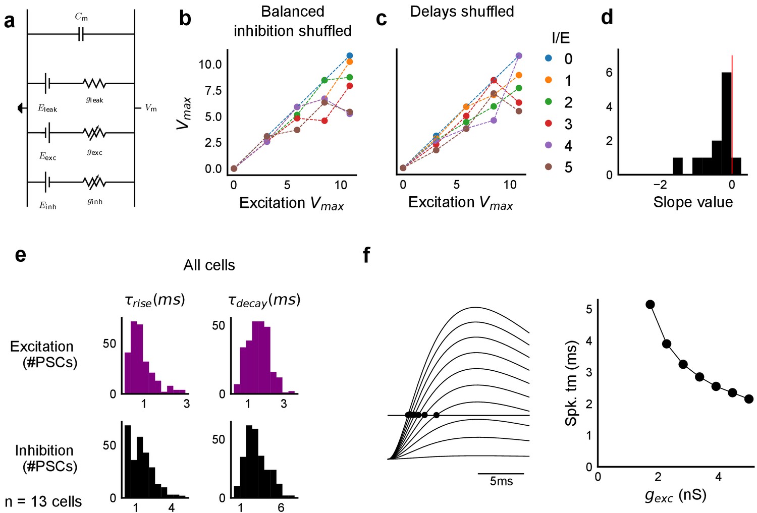
Sensitivity of SDN to EI balance and EI delay, and synaptic time courses used for model.
(a) Equivalent circuit for the conductance model showing capacitive, excitatory, inhibitory, and leak components. (b,c) Subthreshold divisive normalization was sensitive to I/E ratio (b), and EI delay (c). SDN was lost when the relationship between I/E ratios for a given cell was permuted b. SDN was also lost when the relationship of delay to excitation (Figure 6e) was permuted (c). (d) Histogram of slopes of linear regression lines through EI delays () vs excitatory conductance () for cells in Figure 6g. (e) Rise times () and decay times () were extracted from optically evoked postsynaptic currents (EPSCs and IPSCs, Figure 2, Figure 2—figure supplement 1) by fitting a difference of exponentials (Figure 6, Equation (8)) (n = 13 cells). (f) Schematic showing that our observed delay function (right) can be obtained by thresholding of EPSPs (left) in the simple conductance model.
Figure 6—figure supplement 2
HH model simulations with voltage clamped data show SDN.
(a) Fits of parameter γ (Equation (3)) to peak Vm vs excitatory conductance for simulations of the HH model with synaptic conductances taken from voltage clamped cells. Black dots are medians for peak depolarization caused by excitatory conductance paired with inhibitory conductance for 6 repeats of the same stimulus. X-axis conductance values were scaled with a factor of 100 for fitting. (b) Difference in fit parameter γ for the case with and without inhibition, black dots are means. The two distributions were significantly different (Wilcoxon rank sum test, p<1e-4, n = 13). The fit was susceptible to outliers in some cases.
Figure 7 with 1 supplement
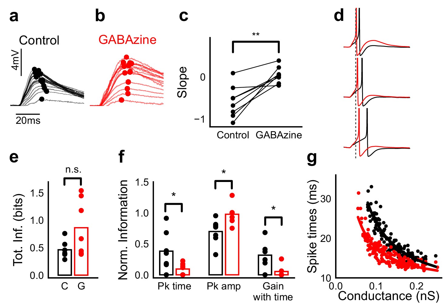
Advancing inhibitory onset changes PSP peak time and spike time with increase in stimulus strength.
(a,b) The PSP peak arrived earlier following larger input in the control case (black), but not with GABAzine in bath (red). Traces for an example cell, binned (20 bins for Expected sum axis) and averaged, for control (black) and with GABAzine in bath (red). (c) Slope of the peak time was more negative in presence of inhibition (control) than when inhibition was blocked (GABAzine) (n = 8 cells). (d) Three example traces from the cell in g showing the relationship of spikes in presence (black) and absence of inhibition (red). Spikes were produced by HH model, using synaptic conductances from voltage clamp data. The separation between spike times of the two conditions increased with decrease in input conductance (top to bottom). (e) Total mutual information of peak amplitude and peak timing with expected sum was not significantly different between Control and GABAzine case (Wilcoxon Rank sum test (<0.05), p=0.11, n = 7 CA1 cells). (f) Normalized mutual information between Expected Vm and peak time, Expected Vm and peak amplitude, and conditional mutual information between Expected Vm and peak time, given the knowledge of peak amplitude. Normalized information was calculated by dividing mutual information by total information for each cell (as shown in d). Peak times carried more information in the presence of inhibition, and peak amplitudes carried more information in the absence of inhibition. There was higher gain in information about the input with timing if the inhibition was kept intact (Wilcoxon Rank sum test (p<0.05), n = 7 (Pk time, Pk amp) and (p=0.05) n = 6 (Gain with time) CA1 cells). (g) Relationship of spike time with excitatory conductance, in the presence (black) and absence of inhibition (red), for HH model simulations. All black points are medians of spikes of each excitation trace paired with six different repeats of inhibition for that combination.
Figure 7—figure supplement 1
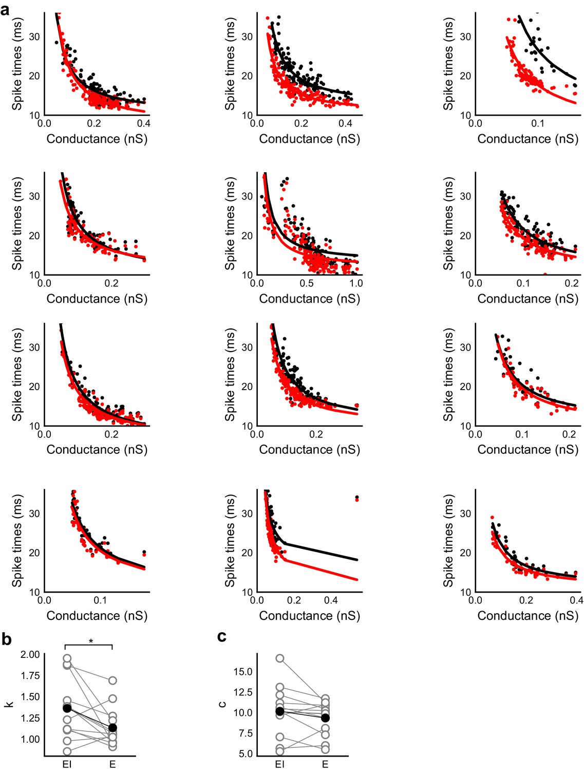
Spike time changes with increasing input are steeper in presence of inhibition.
(a) Plots from HH model, simulated using data from voltage clamp cells, show the relationship of spike time with conductance, with (black) and without inhibition (red). Each plot is produced using data from an individual cell. Each black point is the median of spike times evoked by excitation paired with six different repeats of inhibition for that stimulus combination. Red points are spike times produced for the same values of excitation, but without any inhibition. Separation of the curves was strongly dependent on the exact value of threshold. Using the natural threshold which emerged from the HH model (−56.3 mV), separation could be seen for about half the cells. (b,c) Value of fit parameters k,c when the relationship between spike times and excitatory were fit by c + k/x curve. There was significant difference (Wilcoxon rank sum test, p<0.05, n = 13) between the steepness of the curves for the cases with and without inhibition, where the absence of inhibition makes this curve steeper. There was no significant difference between the intercepts for these fits (Wilcoxon rank sum test, p>0.05, n = 13).
Figure 8 with 1 supplement
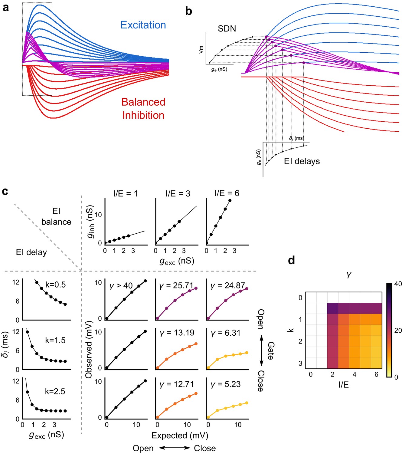
Emergence of SDN from balanced excitation and inhibition, coupled with dynamic EI delays.
(a) Schematic showing precisely balanced EPSPs (blue) and corresponding IPSPs (red) summing to produce PSPs (purple). The EPSPs and IPSPs increase in equal input steps. (b) Zooming into the portion in the rectangle in a. Excitation onset is constant, but inhibition onset changes as an inverse function of input or conductance (), as shown in Figure 6. With increasing input, inhibition arrives earlier and cuts into excitation earlier for each input step. This results in smaller differences in excitatory peaks with each input step, resulting in SDN. The timing of PSP peaks (purple) becomes progressively advanced, whereas the timing of EPSP peaks (blue) does not, consistent with our results in Figure 7. (c,d) Normalization as a function of the two building blocks – EI balance (I/E ratio) and EI delays (interneuron recruitment kinetics, k, as predicted by the model. Larger values of both imply greater normalization and increased gating. Colors of the SDN curves depict the value of gamma (γ), as shown in the phase plot in d. White squares are values of γ larger than 40, where almost no normalization occurs.
Figure 8—figure supplement 1
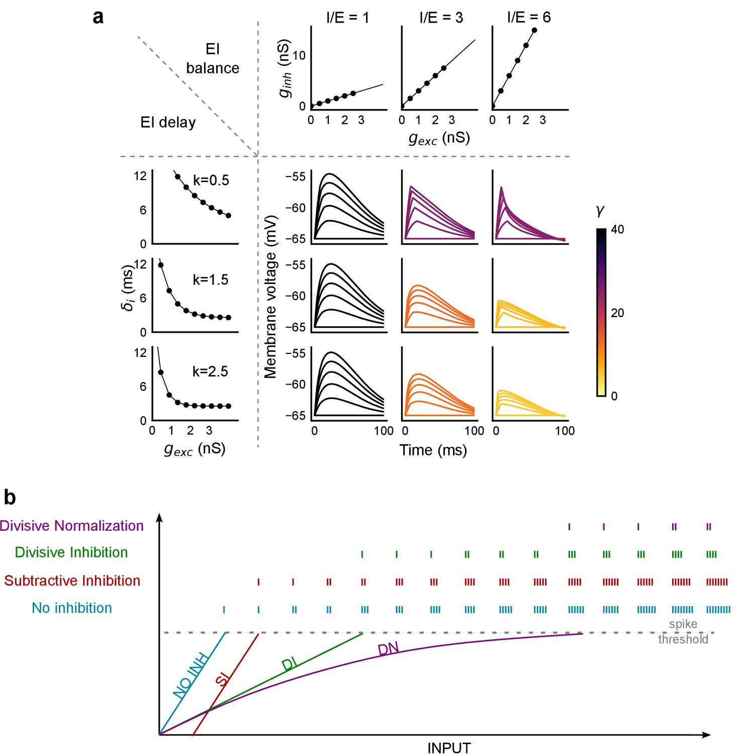
PSP traces showing the effect of I/E ratio and inhibitory recruitment kinetics (k) on SDN.
(a) Similar to Figure 8c, but with the simulated membrane potential traces replacing the Input-Output curves. Colorbar represents values of γ. (b) Input range expansion by SDN. Schematic shows comparison of various models of EI interaction for the range of inputs accommodated by a neuron, before reaching spike threshold.
Videos
Video 1
Subthreshold divisive normalization emerges when onset delay of balanced inhibition dynamically decreases with excitation.
(a) Schematic of the model of a single compartment neuron, which receives excitatory stimulus (in blue) at 20 ms, followed by an inhibitory stimulus (in orange) with variable onset delays. (b) Excitatory conductance (gluGbar) changes as shown in top most slider. Inhibitory conductance (I/E ratio*gluGbar) arrives after a dynamic or static delay. The orange and the blue dotted lines track the inhibition onset and the excitation peak, respectively. Their interaction point, marked by the orange dot, traces the relationship of excitatory conductance with dynamic or static delay. (c) EI summation plot (Figures 3d and 4b) of PSP peak against excitation. Model shows SDN with dynamic EI delays, characterized by the initial linear zone followed by a sublinear zone for higher excitation values. SDN was lost when the EI delay was static. (d) Membrane voltage change as a result of only excitatory (dotted line), and integration of excitatory and inhibitory conductances (solid line) from panel b. Note how the peak time changes as a function of delays.
Tables
Key resources table
| Reagent type (species) or resource | Designation | Source or reference | Identifiers | Additional information |
|---|---|---|---|---|
| Genetic reagent (M. musculus) | C57BL/6-Tg(Grik4-cre)G32-4Stl/J | Jackson Laboratory | Stock #:006474 | Dr. Susumu Tonegawa's laboratory, MIT |
| Strain, strain background (Adeno-associated virus) | AAV5.CAGGS.Flex.ChR2-tdTomato.WPRE.SV40 | Penn Vector Core | ||
| Software, algorithm | MOOSE simulator | Ray and Bhalla, 2008 | RRID:SCR_008031 | Dr. Upinder Bhalla's laboratory, NCBS |
Additional files
-
Supplementary file 1
Table S1 Synaptic time courses chosen for the model.
The median, 25% and 75% values for each of the four distributions in Figure 6—figure supplement 1e are shown.
- https://cdn.elifesciences.org/articles/43415/elife-43415-supp1-v3.docx
-
Supplementary file 2
Table S2 Parameters for the conductance model.
Parameters for this model were either calculated using electrophysiological experimental conditions, taken from literature (Table S2a) or fit from data (Table S2b).
- https://cdn.elifesciences.org/articles/43415/elife-43415-supp2-v3.docx
-
Supplementary file 3
Table S3 Parameters for the HH based conductance model.
Parameters for this model were either calculated using electrophysiological experimental conditions, or taken from literature. The simulations were conducted using synaptic conductances, measured from voltage clamp data (Figure 2).
- https://cdn.elifesciences.org/articles/43415/elife-43415-supp3-v3.docx
-
Transparent reporting form
- https://cdn.elifesciences.org/articles/43415/elife-43415-transrepform-v3.pdf
Download links
A two-part list of links to download the article, or parts of the article, in various formats.
Downloads (link to download the article as PDF)
Open citations (links to open the citations from this article in various online reference manager services)
Cite this article (links to download the citations from this article in formats compatible with various reference manager tools)
Precise excitation-inhibition balance controls gain and timing in the hippocampus
eLife 8:e43415.
https://doi.org/10.7554/eLife.43415


