Rapid task-dependent tuning of the mouse olfactory bulb
Figures
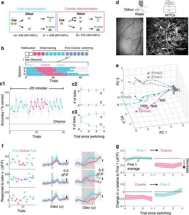
OB output neurons change olfactory representation rapidly and reproducibly with demands.
(a) Structure of discrimination tasks. (Left) Fine discrimination. A trial starts with two flashes of an LED. A rewarded stimulus (α) is a mixture of A and B odours at a concentration ratio of 40:60% (α-odour), associated with a water (reward). In a non-rewarded trial, the A/B mixture is presented at a concentration ratio of 60:40% (α’-odour), and no reward is given. (Right) Coarse discrimination. A trial starts with one flash of an LED. The rewarded odour is the same A/B 40/60 mixture as in fine discrimination. A non-rewarded stimulus is a mixture of different odours (β). On some rewarded trials, α’ odour is presented to assess whether mice generalize across both A/B mixtures. (b) Timeline of experiment. Each session lasted ~20 min, and occurred once a day. Inset: Example of switching sessions used for a typical animal (six sessions shown). Variable epoch length ensures that at least four rewarded trials appear per epoch. (c) Trial-by-trial average performance across five mice for all trials (c1), as well as trials around switching (c2,c3). Mean and s.e.m. are shown. (d) Imaging configuration. GCaMP6f fluorescence from mitral and tufted cells was imaged with a two-photon microscope through a chronic window (middle) in head-fixed mice performing task switching. Right, an example field of view. Scale bar = 50 μm. (e) Trajectories corresponding to the α and α’ odours during fine and coarse discrimination, plotted as trajectories in the first three principal components. Pseudo-population response constructed from all ROIs (n = 353, five mice). (f) Left, Trial-by-trial α odour response (average amplitude during 1 s odour presentation) for example ROIs. Mean and s.e.m. are shown as horizontal lines. Middle, Corresponding transients averaged for each task type. Right, The same traces as in the middle panel, but zoomed into the odour period. (g) Time course of change among significantly modulated ROIs. The response amplitude for an odour relative to response amplitudes during the first fine discrimination epoch (mean ±s.e.m.; n = 42 ROIs, five mice). The observation holds true when the rewarded trials are not preceded by a non-rewarded trial (data not shown).
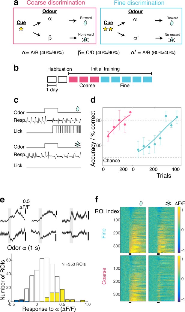
Method for imposing different behavioural task demands.
(A) Structure of discrimination tasks. Right, Fine discrimination. A trial starts with two flashes of an LED. The rewarded stimulus (α) is a mixture of A and B odours at a concentration ratio of 40:60% (α-odour), associated with a water reward. In a non-rewarded trial, the A/B mixture at a concentration ratio of 60:40% (α’-odour) is presented, but no reward is given. Left, Coarse discrimination. A trial starts with one flash of an LED. The rewarded odour is the same as in fine discrimination. A non-rewarded stimulus is a mixture of different odours (β). In some rewarded trials, α’ odour is presented to assess whether mice generalize across both A/B mixtures. (B) Schematic showing timeline of initial training before mice were subjected to switch training. Each box represents one session, which occurred once a day. Following two days of habituation, mice went through on average three sessions of coarse discrimination training and five sessions of fine discrimination training. (C) Examples of correct behavioural responses for rewarded trials (top; correct hit) and for non-rewarded trials (bottom; correct rejection). An odour is presented for 1 s. and a reward is delivered 3 s after onset of the odour. (D) Learning rates for head-fixed mice used in the experiment (n = 5 mice) corresponding to initial training days as in (B). Mean and s.e.m. shown. (E) Above. Examples of excitatory and inhibitory responses evoked by S+ odour (gray bar, 1 s). Below. The distribution of responses evoked by S+ odour. Yellow and blue bars = significantly excitatory and inhibitory responses, respectively (see Materials and methods under ‘Odour response’). Scale bar, 0.5 ΔF/F. (F) Calcium transients as color maps in response to rewarded (left) and non-rewarded (right) odours for the tasks indicated. ROIs are sorted by the S+ response amplitude. n = 353 ROIs, five mice.
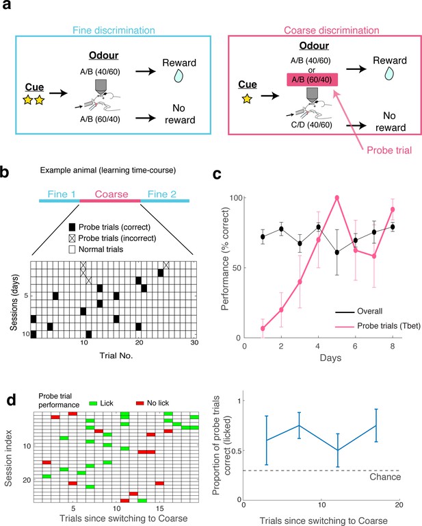
Task-switch learning and probe trials.
(A) Behavioural paradigm for task switching. Mice are trained to perform fine discrimination blocks before and after a coarse discrimination block within one session. The design of the coarse discrimination is such that mice are forced to generalise closely related odours. On a given rewarded (S+) trial, the odour was either A/B in a 40/60 mixture or A/B in a 60/40 mixture. This latter stimulus appears as the non-rewarded odour in the fine discrimination session. Therefore, the A/B (60/40) trial during the coarse discrimination block serves as a test to see whether mice genuinely perform tasks differently, so they are termed ‘Probe trials.’ (B) A typical example showing the performance of a mouse during the probe trials over several days (one session per day). Trials during coarse discrimination are shown as tiles. Probe trials with an incorrect response (i.e., no lick) are marked with a cross, while those with a correct response are shown as filled tiles. (C) On average, mice learned to perform task-switching in 4 days, as seen in the performance accuracy in these probe and overall trials. N = 5 mice for Tbet-Cre x Ai95D experiment (average of 1.6 ± 0.4 trials per mouse per session). (D) Switch performance for all trials used in the imaging sessions (five mice). Trials are shown from the time of switching from fine discrimination epoch one to coarse discrimination. Left: The lick performance for each probe trial is colour-coded, where green indicates the presence of lick (significantly more than during the baseline period, based on Poisson distribution of lick count during the baseline period), and red indicates the absence of lick in response to α’-odour presentation. Right: Summary showing the average lick performance on probe trials binned into 4 phases of coarse discrimination epoch. Chance level is the average probability of observing a lick in response to a’-odour during fine discrimination epochs. Mean and s.e.m. shown (average of zeros and ones, with each point reflecting approximately seven trials).
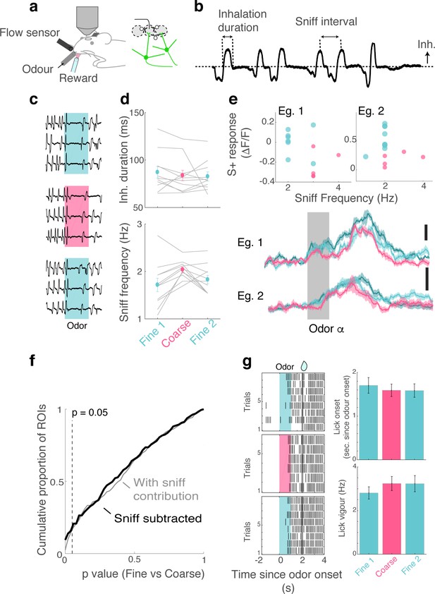
Movement and sniff patterns do not contribute to task-dependent differences.
(A) Experimental setup. A flow sensor was placed in close proximity to the right nostril to monitor respiratory rhythms while the odour was presented to the left nostril. A lick sensor was a small beam break sensor placed around a water delivery port. (B) Explanation of sniff parameters measured. (C) Example of respiratory traces around the time of odour presentation. Inhalation is plotted upwards. (D) Summary of sniffing patterns showing the average duration of inhalation (above) and the number of inhalations taken during the 1 s odour presentation (below). (E) Examples of dependence on sniff: odour-evoked response amplitudes of two example ROIs against sniff frequency for individual trials during fine discrimination (turquoise) and coarse discrimination (magenta). Average transients for the same ROIs (below). (F) Distribution of p-values where dependency on sniff frequency is eliminated thorough linear regression (fitted for rewarded odour responses during fine discrimination) in black, and overall p-value distribution where sniff contribution is not subtracted (gray). (G) Lick patterns following rewarded odour presentation. Left, Examples from one imaging session. Ticks represent occurrence of licks. Each tick represents the onset of licking, relative to the onset of odour presentation. Right, Summary showing the timing of the first lick after odour onset (above) and frequency of licking for a 3 s window before reward delivery (below).
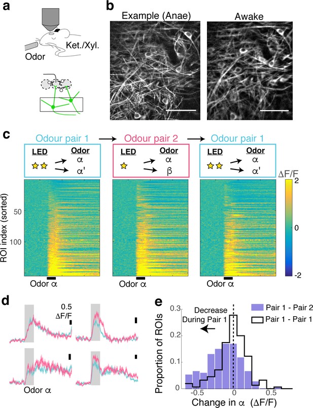
Task-dependent modulation observed during behaviour is absent under anaesthesia.
(A) After the behavioural experiments, mice were anaesthetized with ketamine and xylazine (i.p.). (B) Example fields of view from an example animal show the same location imaged during anaesthesia (left) and during behavioural experiment (right). Scale bar = 50 μm. (C) Calcium transients for 155 ROIs imaged, in response to the same rewarded odour. (D) Average transients from four example ROIs in response to the rewarded odour during fine (turquoise) and coarse (magenta) stimulus presentations. Scale bar = 0.5 ΔF/F. (E) Histogram of task-dependent change in α odour responses (response during fine discrimination – response during coarse discrimination).
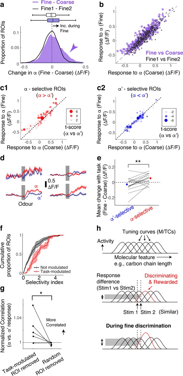
Selective amplification leads to demand-specific enhancement of stimulus decorrelation.
(a) Histogram of task-dependent change in α responses (response during fine discrimination – response during coarse discrimination; purple). Within-task variability (black line) is shown for comparison. (b) Comparison of odour responses during coarse (x-axis) and fine (y-axis) discrimination for all ROIs (purple). Within-task comparison (Fine1 vs Fine2; black points) shown for reference. (c) Task-dependent odour response comparison as in (b), but separated by odour selectivity. α-selective ROIs (red) are ROIs with t-scores greater than zero, where the strength of the selectivity is indicated by the size of the marker. α‘- selective ROIs are those with t-scores <0. (d) Average transients in response to odour α (red) and odour α’ (blue) from 4 ROIs selective for odour α. Error bar = s.e.m. (e) Summary of task-dependent change for odour α for ROIs grouped by selectivity. Each data point = average for each imaged location. N = 21 sessions, five mice. Sessions where probe trials were omitted are excluded from this analysis. (f) Distribution of selectivity indices for task-modulated ROIs (red; n = 32 ROIs, five mice) and ROIs without task modulation (black; n = 255 ROIs, five mice). The selectivity index is the absolute value of the t-score for α-responses vs α’-responses imaged during fine discrimination. (g) Correlation coefficients between α vs α’ responses, where a subset of ROIs is removed and normalized to when a full set of ROIs used. Each coefficient is from ROIs from individual animals, instead of imaging location, due to a small number of ROIs in some imaged locations (n = 5 mice). (h) Schematic of finding. MTCs tuned to different ‘molecular features,’ for example, distinct carbon chain lengths, have different tuning curves along this axis. Some MTCs respond differently to two similar stimuli (stim 1 and stim 2), which contribute the most to discrimination. MTCs that are selectively tuned to the rewarded odour are enhanced when mice need to discriminate between the two similar odours, resulting in enhanced discriminability.
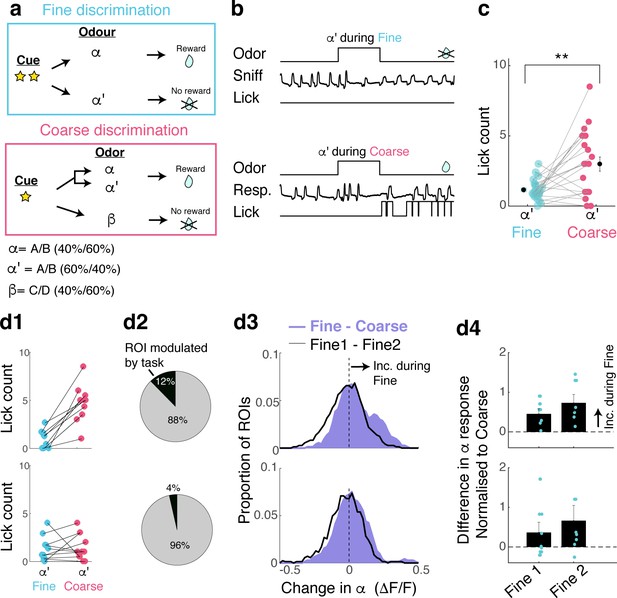
Task-related change is prevalent in sessions with clear evidence of switching.
(A) Task structures as before. (B) Example of trials where a 60A/40B mixture (α’ odour) was presented as a non-rewarded odour during fine discrimination (above) and as a rewarded odour during coarse discrimination (below). (C) Summary comparison of lick response for the same odour but during different tasks. (D) Analysis of data from sessions in which mice switched vs those in which they did not. All data are from well-trained animals, with imaging taking place on 3–6 days since the beginning of switch training. (D1) Definition of switching based on licking pattern following α‘ odour presentation. Above: sessions in which mice switched, defined by a significant increase in licking during α‘ trials during coarse discrimination. N = 10 imaging sessions, five mice. Below, Definition of sessions in which mice did not switch, where licking patterns during α ‘odour trials do not differ during fine and coarse discrimination. N = 11 imaging sessions, five mice. (D2) Proportion of ROIs that are modulated by task for sessions with evidence of behavioural switching (above) and sessions with no such evidence (below). N = 146 ROIs and 141 ROIs, respectively. (D3) Histogram of change in α odour response amplitudes, across task (Fine - Coarse discrimination; purple) and within task (Fine1 – Fine2, black line). N = same as in D2. (D4) Task-dependent change in α response amplitudes; summary representing individual imaging sessions (N = 10 for sessions with behavioural switching, n = 11 for sessions with no behavioural switching).
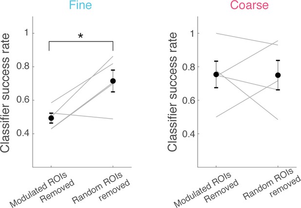
Role of task-modulated neurons in task-dependent stimulus discrimination.
Linear classification performance for discrimination of α vs α’ odours (trials from fine discrimination epochs), where a subset of ROIs is removed. Each success rate plotted is from an individual animal, as in Figure 2g.
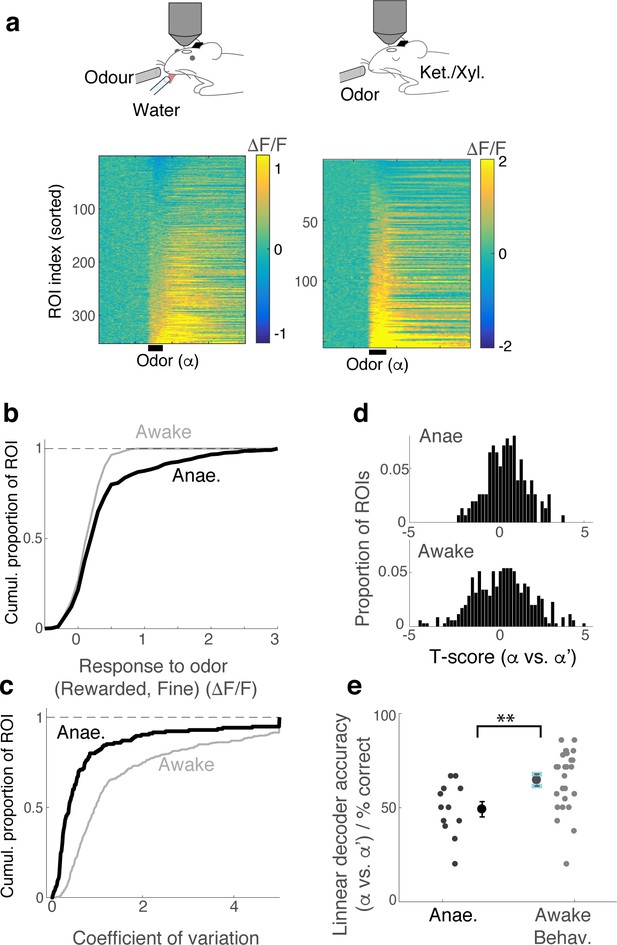
Responses are more reliably discriminated in behaving mice.
(A) GCaMP6f fluorescence change is represented in a color map for 353 ROIs imaged from awake, behaving mice (26 imaging sessions, five mice). Left; Responses are from mice performing the fine discrimination task. Right; Following behavioural experiments, mice were anaesthetized with ketamine/zylazine and M/TCs imaged (12 imaging sessions, three mice). Responses are from block 1, where odour α and odour α’ were presented closely in time. (B,C) Comparison of cumulative histogram of response amplitudes (B) and coefficient of variation (C) for odour α (average during 1 s after valve opening). (D) Comparison of t-score distribution (α odour response vs α’ odour response amplitudes) for ROIs imaged from anaesthetized (above) and awake, behaving (below) mice. (E) For each imaged location, a linear classifier was trained on a subset of α- and α’- trials. Its performance for test trials is shown as % correct. (average accuracy = 49.1 ± 4% correct for anaesthetised vs. 64.6 ± 3.0% correct for awake, behaving case; p=0.006, Wilcoxon rank sum test; n = 12 imaged locations, three mice for anaesthetized mice vs. 26 locations, four mice for awake).
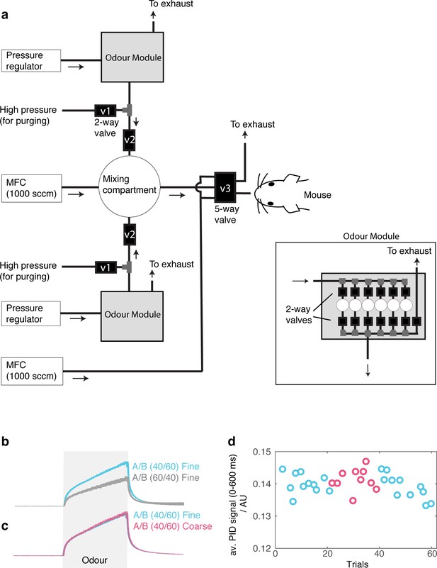
PID signals show stable odour pulses.
(A) Olfactometer design for mixing two odorant streams at desired concentrations for generating binary mixtures. For each odorant, filtered and regulated air is passed through a selected odour canister by opening a pair of two-way solenoid valves ('Odour module'). Odourized air is passed through a second, fast solenoid valve (‘v2’) in a pulsatile manner. Pulses of odourized air are mixed in an enlarged compartment (a 50 ml flask) to remove transients. The odour concentration can be set by controlling background air flow and odorized pulse parameters (duration and frequency of rectangular pulses). Mixed air passes through thin PTFE tubing (O.D., 3.2 mm) and is presented to the animal when the 5-way solenoid valve is actuated. (B) For characterizing the stimulus profile, a photo-ionization detector was placed in front of the odour port, in place of the mouse. Instead of the usual binary mixtures, the test used a mixture of 1 odorised stream and one blank stream (passing air through an empty odour vial) mixed in the same way to test the concentration of each component separately. PID signals from trials where the composition of the tested odour is 60% (cyan) vs 40% (gray), corresponding to the composition of an odour ‘A’ in S+ and S- trials, respectively. (C) Odour concentrations (PID signal) measured during coarse and fine discrimination for the switching paradigm are overlaid. Mean +- standard error of the mean shown (~15 trials each). (D) Time-course of odour concentrations to test the depletion level during a task-switch session. The inter-trial interval was approximately 20 s. Data shown are the average PID signal during the first 600 ms of odour period.
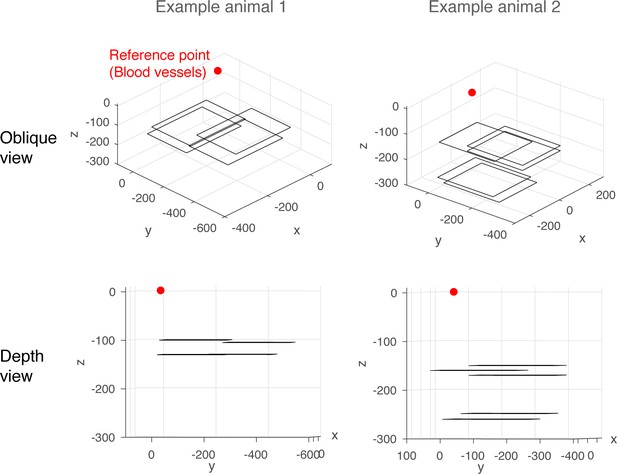
Examples of imaged planes.
For each imaging session, images were obtained from a 256 μm x 256 μm field of view from a single plane. In each animal, imaging sessions took place over multiple sessions, depending on the quality of the optical window, as well as the presence of odour-responsive neurons. The panels show all imaged planes from two example mice, with two viewing angles.
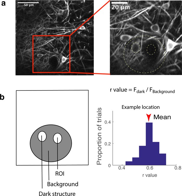
Estimation of contribution from out-of-focus fluorescence.
The method is based on Kerlin et al. Briefly, to estimate how much out-of-focus fluorescence contributes to fluorescence within an ROI, the fluorescence of a neighbouring dark object (Fdark; blood vessel or unstained structure) and the fluorescence of the area surrounding the two objects (ROI and the dark object) are compared. The ratio Fdark/Fbackground is the estimated fractional contribution from out-of-focus fluorescence.
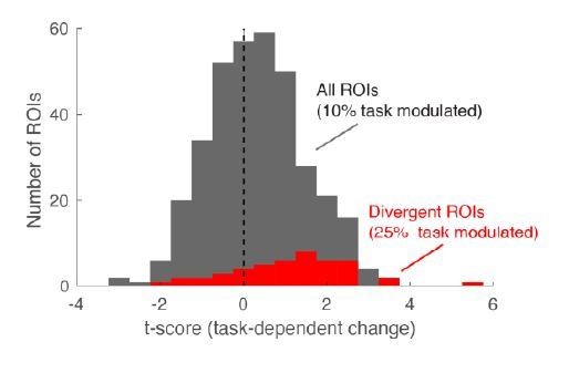
Histogram of task-dependent change, expressed as t-score (fine vs. coarse).
Overall, 10% of neurons change with task. Among the α-selective ROIs (cells responding differently to the 40/60 and 60/40 mixtures) this proportion is substantially higher (25%, red). These α-selective ROIs make up approximately 12% of all ROIs – closely matching published results for divergent cells in a long learning task studied by Chu et al., 2016.
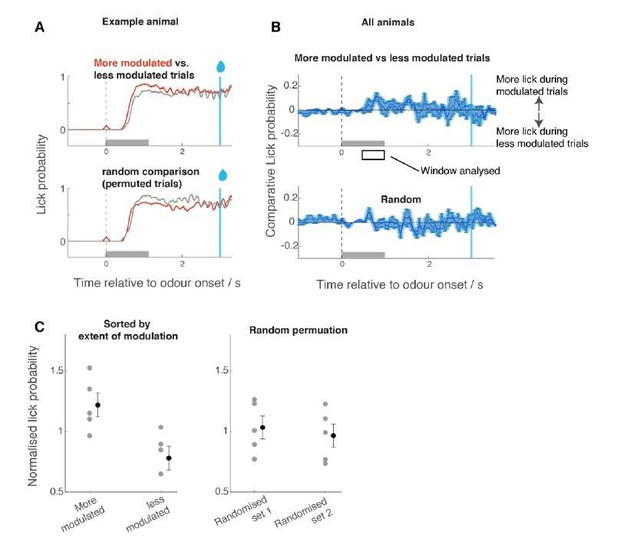
Comparison of licking behaviour for trials with larger modulation vs trials with less modulation.
For each ROI and for each trial, the odour response amplitude was expressed as a t-score (in comparison against the mean response amplitude during coarse discrimination, taking into account the trial-to-trial variability). For each trial, the average t-score across ROIs was determined. Based on this average t-score, the trials were grouped into high- and low-modulation groups, and the corresponding licking waveforms were extracted (A,B). Mean lick probability was measured for the time window indicated with a rectangle in B, and normalized by the average lick probability for all trials. For control, trial order was randomized but otherwise the same analysis was carried out.
Additional files
-
Transparent reporting form
- https://doi.org/10.7554/eLife.43558.014


