Long-term balancing selection drives evolution of immunity genes in Capsella
- Max Planck Institute for Developmental Biology, Germany
- Stockholm University, Sweden
- University of Osnabrück, Germany
- University of Toronto, Canada
Figures
Figure 1 with 1 supplement
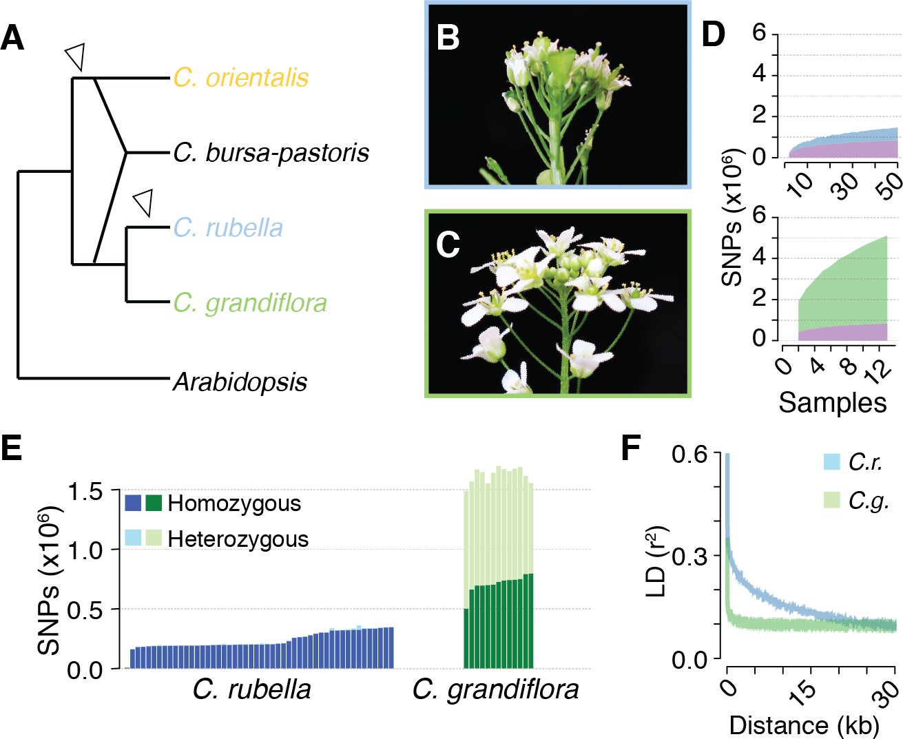
Polymorphism discovery in Capsella.
(A) Diagram of the relationships between Capsella species. Arrowheads indicate transitions from outcrossing to self-fertilisation. (B) Inflorescence of C. rubella with small flowers. (C) Inflorescence of C. grandiflora with large, showy flowers, to attract pollinators. (D) SNP discovery in C. rubella (top) and C. grandiflora (bottom). Samples were randomly downsampled ten times. Means of segregating transpecific (tsSNPs, purple), species specific in C. rubella (ssCrSNPs, blue), and species specific in C. grandiflora (ssCgSNPs, green) SNPs. (E) Number of heterozygous (light colours) and homozygous SNP calls (dark colours). (F) Average decay of linkage disequilibrium in C. grandiflora (green) and C. rubella (blue).
-
Figure 1—source data 1
Sample information.
- https://doi.org/10.7554/eLife.43606.005
-
Figure 1—source data 2
Diversity and divergence estimates for C.grandiflora and C. rubella.
- https://doi.org/10.7554/eLife.43606.006
Figure 1—figure supplement 1
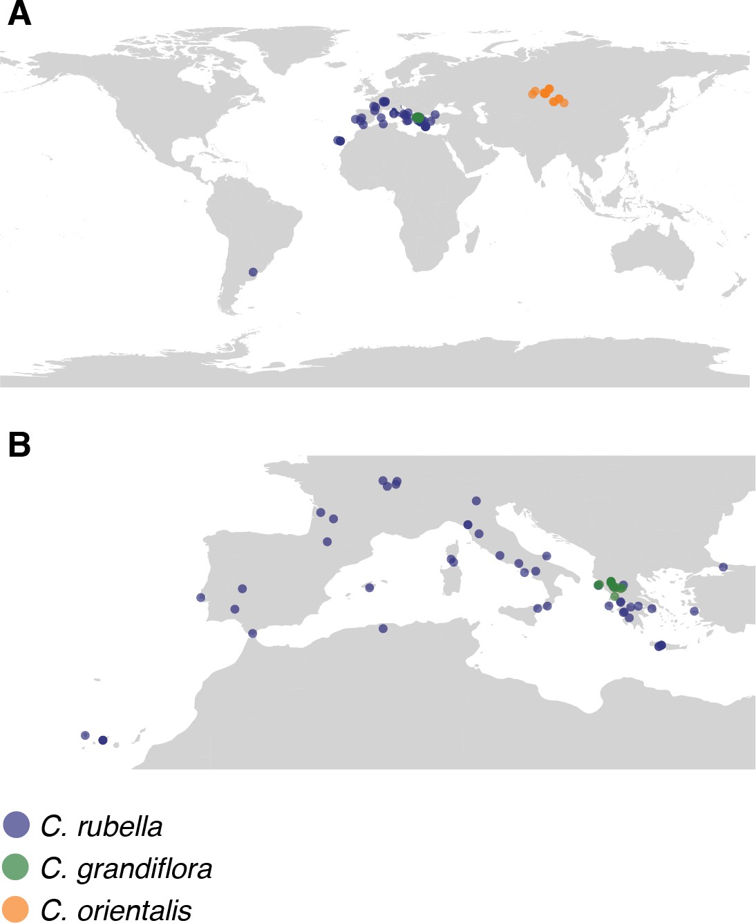
Map of collections.
(A) Global and (B) European locations of samples.
Figure 2 with 2 supplements
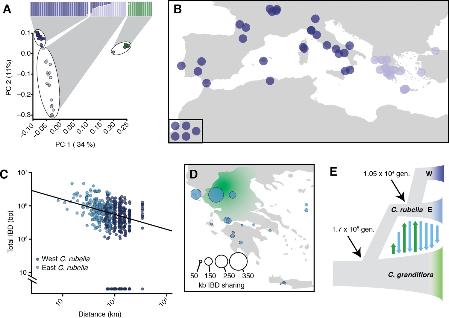
Demographic analysis of C.rubella.
(A) Admixture bar graphs (top) and PCA of population structure in C. grandiflora (green) and C. rubella (blue). The C. rubella colours correspond to the sampling locations in (B). Inset shows lines from outside Eurasia (Canary Islands and Argentina). (C) Pairwise interspecific identity-by-descent (IBD) between C. grandiflora and C. rubella samples. Comparisons between West C. rubella and C. grandiflora are in dark blue and E C. rubella and C. grandiflora in light blue. The minimum segment length threshold was 1 kb, and comparisons without IBD segments (all from the West C. rubella population) are at the bottom of the plot. (D) Total lengths of interspecific IBD sharing by sample site within the E C. rubella population. An approximate distribution of C. grandiflora is shown for comparison in green. (E) The most likely demographic model of C. rubella and C. grandiflora evolution as inferred from joint allele frequency spectra by fastsimcoal2. Arrows indicate gene flow.
-
Figure 2—source data 1
D statistics comparing East and West C.rubella populations.
- https://doi.org/10.7554/eLife.43606.010
-
Figure 2—source data 2
Inferred demographic parameters from fastsimcoal2.
- https://doi.org/10.7554/eLife.43606.011
Figure 2—figure supplement 1
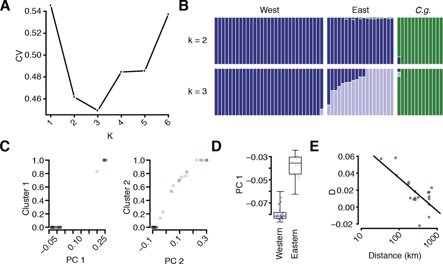
Additional population structure and migration analyses.
(A) Coefficient of variation for different numbers of k in ADMIXTURE runs. (B) Comparison of k = 2 and k = 3 results. (C) Correlation of sample position along PC1 and assignment to the C. grandiflora cluster and along PC2 and assignment to the East C. rubella cluster. (D) Position of East and West C. rubella samples along PC1. Dots show raw values. (E) D statistic in E C. rubella as a function of distance from northern Greece, where C. grandiflora occurs at the highest density. The line depicts a linear regression of this relationship (p<<0.01).
Figure 2—figure supplement 2

Comparison of simulated and observed allele frequency spectra under the best fitting demographic model.
The fit of a simulated jMAF spectrum to the observed data using the most likely demographic model inferred by fastsimcoal2. Heatmaps in the top two rows show the number of mutations falling into a particular frequency class (the minor allele is assigned based on the allele frequency across both populations), while the bottom two rows indicate the residuals of the real data from the simulated (ndata-nmodel)/nmodel.
Figure 3 with 9 supplements
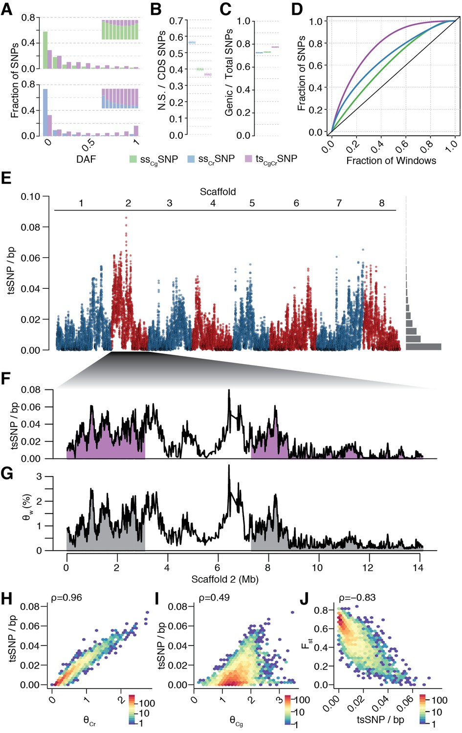
Unequal presence of ancestral variation in modern C.rubella.
(A) Derived allele frequency spectra (DAF) of ssCgSNPs (green), ssCrSNPs (blue), and tsCgCrSNPs (purple) in C. grandiflora (top) and C. rubella (bottom). The inset depicts the fraction of alleles that are species or transpecific as a function of derived allele frequency (DAF). (B) Fraction of coding (CDS) SNPs that result in non-synonymous changes as a function of SNP sharing. (C) Fraction of genic SNPs as a function of SNP sharing. Because SNPs in different classes (ssSNPs, tsSNPs) differ in allele frequency distributions, we normalised by downsampling to comparable frequency spectra. Each bar consists of 1000 points depicting downsampling values. (D) 20 kb genomic windows required to cover different fractions of ssSNPs and tsSNPs. The black line corresponds to a completely even distribution of SNPs in the genome. tsSNPs deviate the most from this null distribution. (E) tsCgCrSNP density in 20 kb windows (5 kb steps) along the eight Capsella chromosomes. Histogram on the right shows distribution of values across the entire genome. (F) tsCgCrSNP density and (G) Watterson’s estimator (Θw) of genetic diversity along scaffold 2. The repeat dense pericentromeric regions are not filled. (H–J) Correlation of tsCgCrSNP density in 20 kb non-overlapping windows with genetic diversity in C. rubella (H), genetic diversity in C. grandiflora (I), and interspecific Fst (J). Spearman’s rho is always given on the top left. Only windows with at least 5000 accessible sites in both species were considered.
Figure 3—figure supplement 1
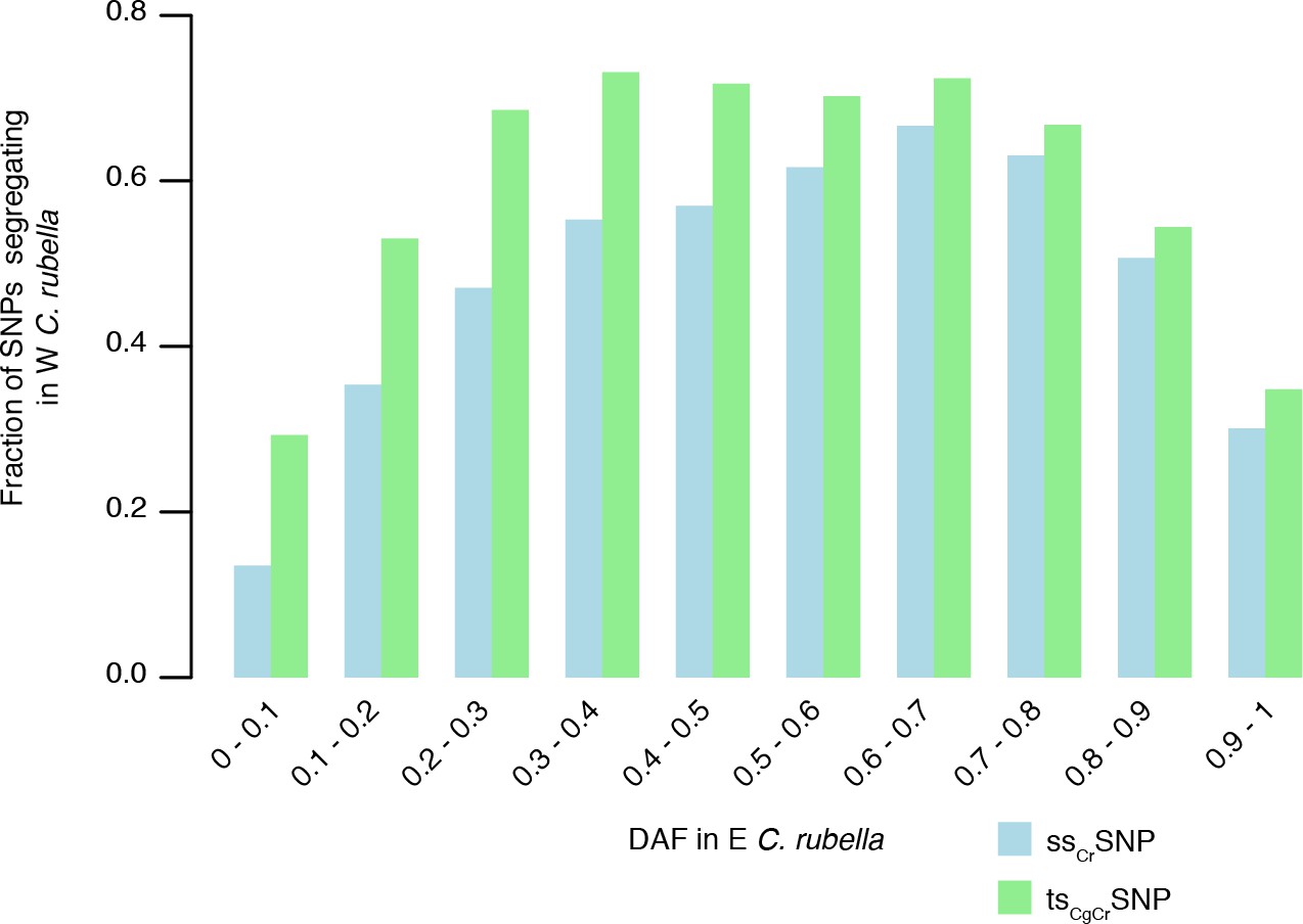
Sharing of tsCgCrSNPs and ssCrSNPs alleles after colonisation.
https://doi.org/10.7554/eLife.43606.013
Figure 3—figure supplement 2
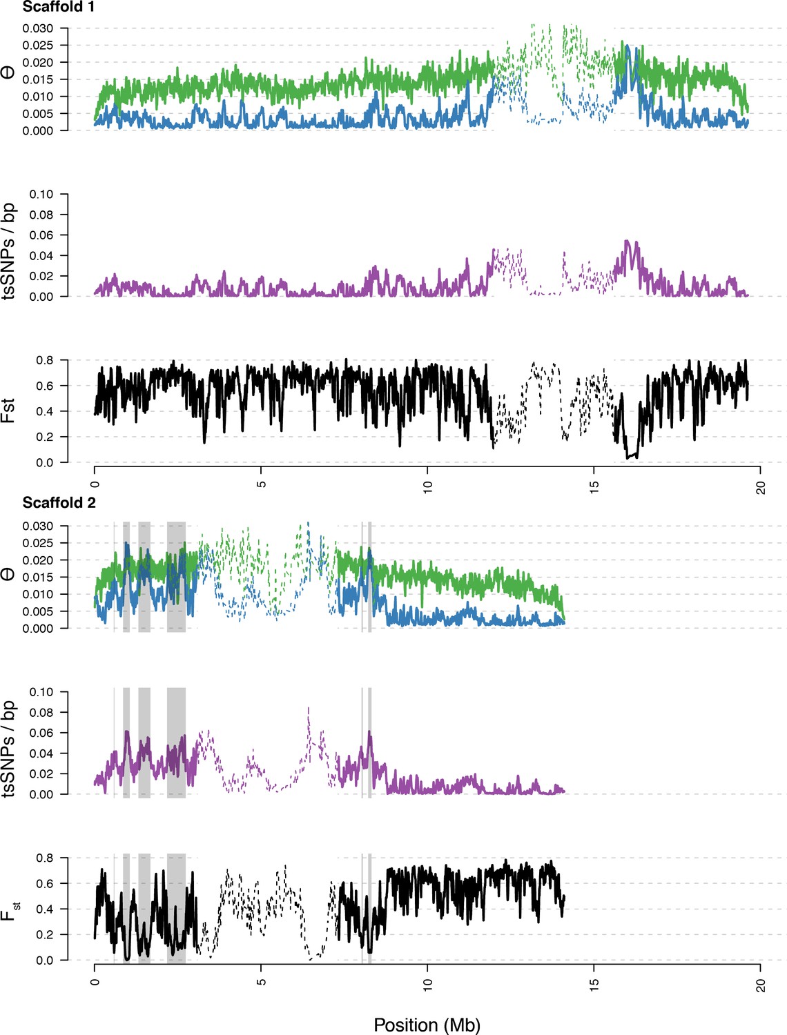
Diversity in C. rubella and C. grandiflora along scaffolds (chromosomes) 1 and 2.
Data calculated in 20 kb windows, 5 kb steps. Windows with fewer than 5000 covered sites were masked for all calculations. Dotted lines indicate the pericentromeric regions excluded from our analysis, and shaded regions highlight the regions with significant evidence for balancing selection.
Figure 3—figure supplement 3
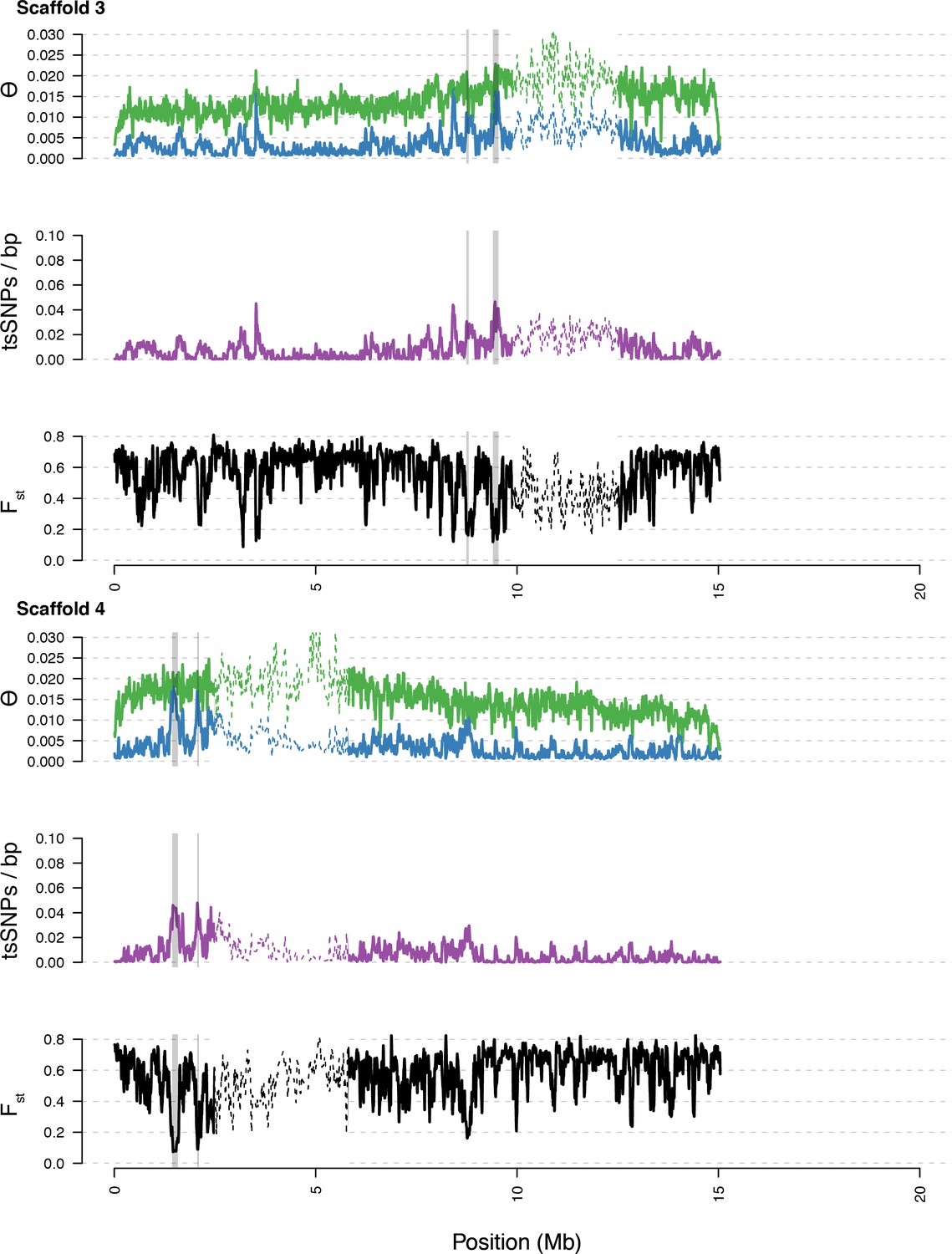
Diversity in C. rubella and C. grandiflora along scaffolds (chromosomes) 3 and 4.
https://doi.org/10.7554/eLife.43606.015
Figure 3—figure supplement 4
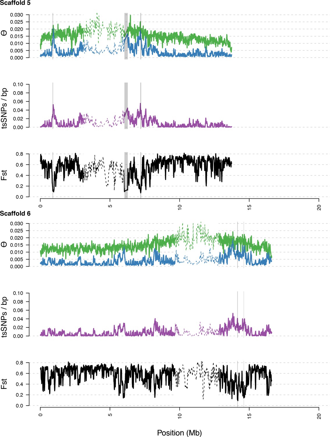
Diversity in C. rubella and C. grandiflora along scaffolds (chromosomes) 5 and 6.
https://doi.org/10.7554/eLife.43606.016
Figure 3—figure supplement 5
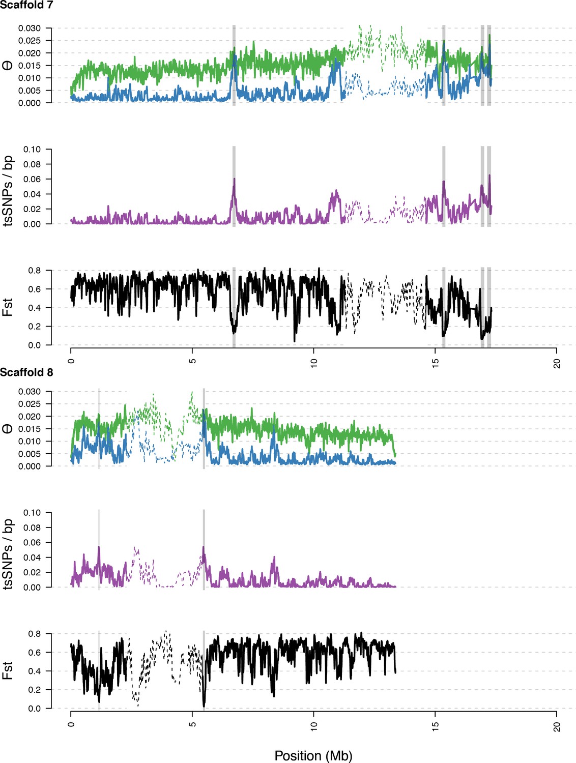
Diversity in C. rubella and C. grandiflora along scaffolds (chromosomes) 7 and 8.
https://doi.org/10.7554/eLife.43606.017
Figure 3—figure supplement 6
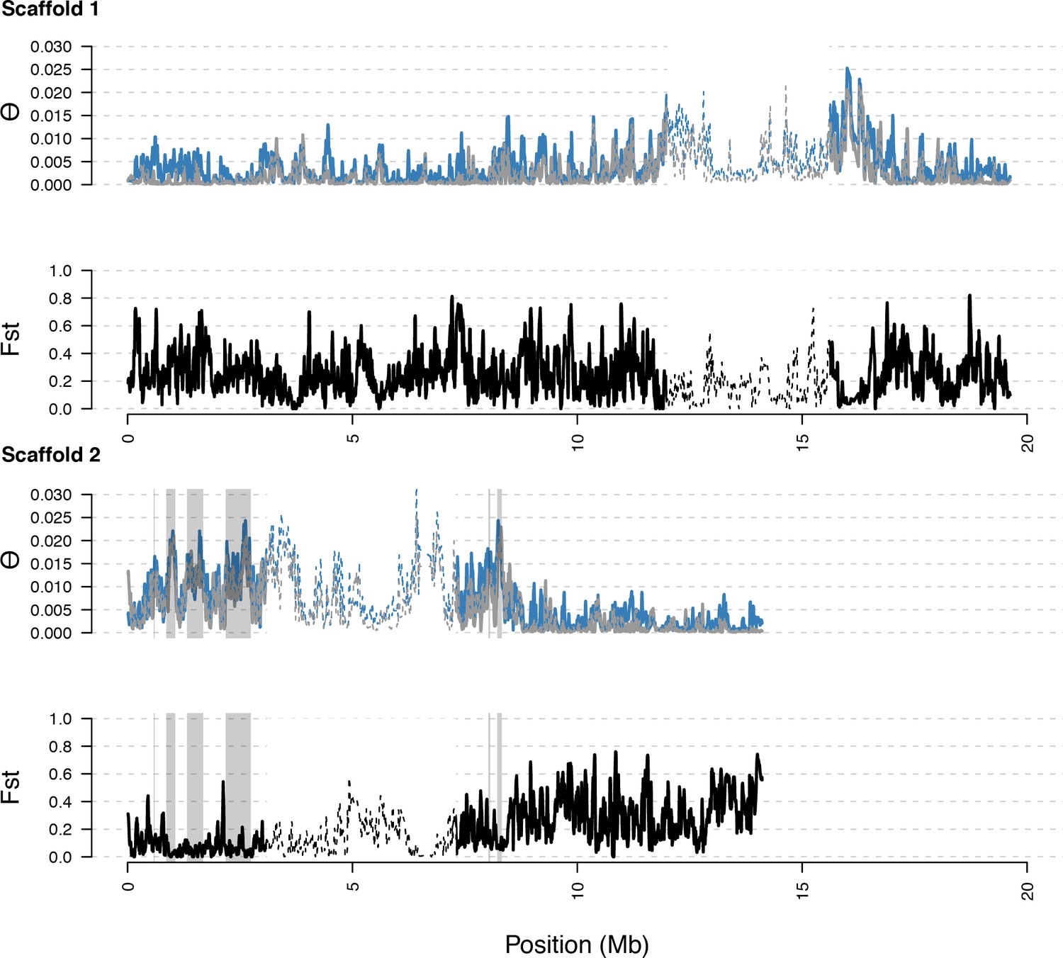
Distribution of diversity in East and West C. rubella populations along scaffolds (chromosomes) 1 and 2.
As in S5, with diversity calculated within and Fst between populations. In general, regions of high diversity species-wide show high diversity and low Fst.
Figure 3—figure supplement 7

Distribution of diversity in East and West C. rubella populations along scaffolds (chromosomes) 3 and 4.
https://doi.org/10.7554/eLife.43606.019
Figure 3—figure supplement 8
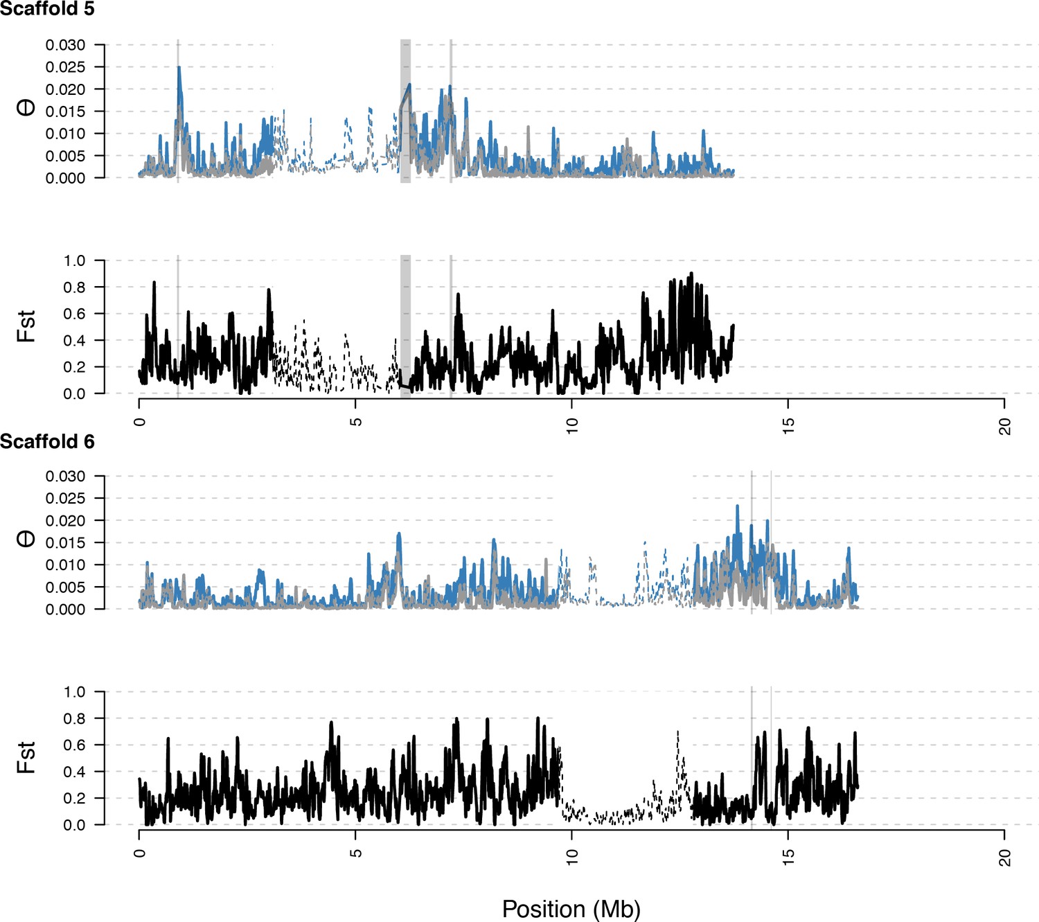
Distribution of diversity in East and West C. rubella populations along scaffolds (chromosomes) 5 and 6.
https://doi.org/10.7554/eLife.43606.020
Figure 3—figure supplement 9
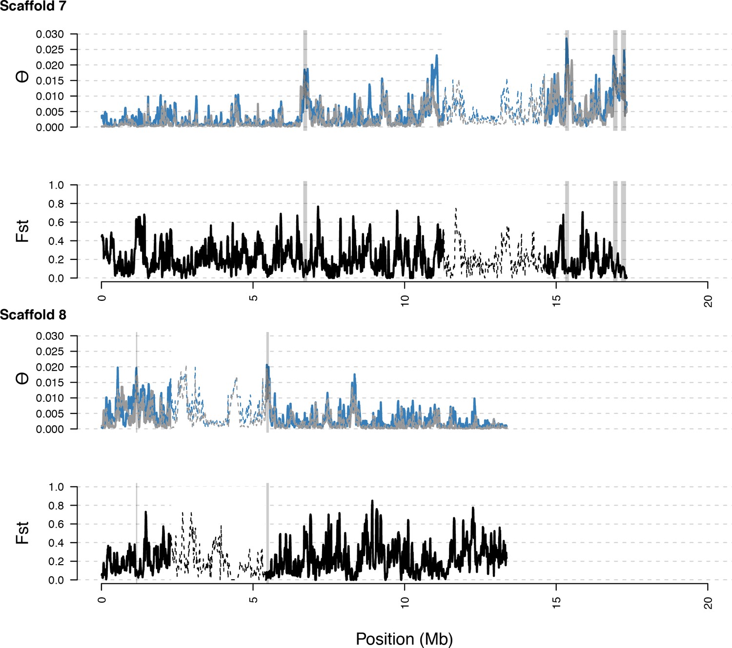
Distribution of diversity in East and West C. rubella populations along scaffolds (chromosomes) 7 and 8.
https://doi.org/10.7554/eLife.43606.021
Figure 4 with 2 supplements
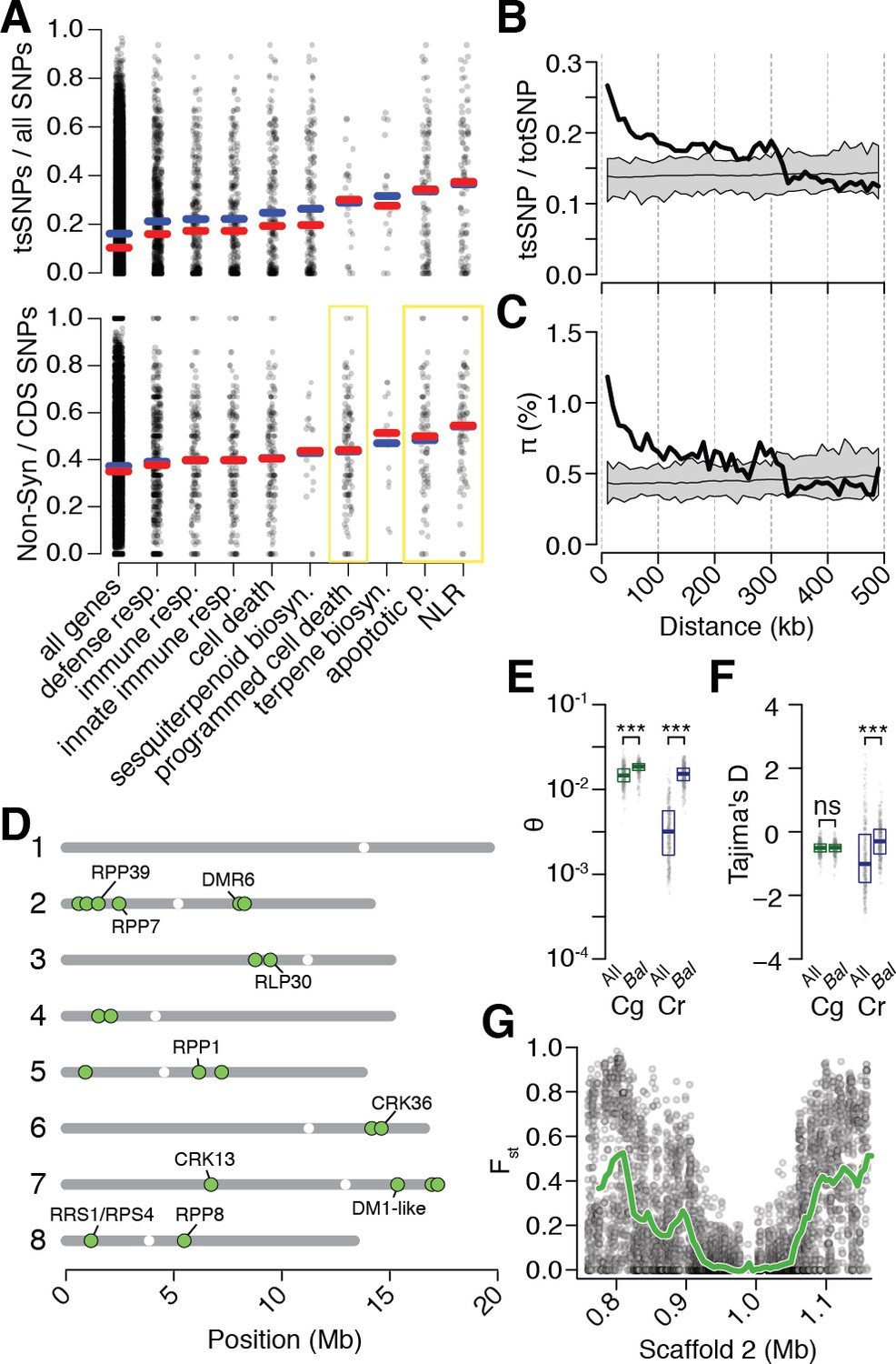
Preferential sharing of alleles near immunity genes.
(A) Enrichment of tsCgCrSNPs and non-synonymous tsCgCrSNPs for genes associated with significant GO terms (means, blue; medians, red). Each point represents values calculated for an individual gene. For example, in the upper subplot each point is the number of tsSNPs identified in a gene divided by the total number of SNPs identified for a gene. GO terms with a significantly increased ratio of nonsynonymous changes are highlighted with a yellow box. (B) tsCgCrSNP frequency as a function of distance to the closest NLR cluster. (C) Pairwise genetic diversity at neutral (four-fold degenerate) sites as a function of distance to the closest NLR cluster. For (B–C) the thick black lines are mean values calculated in 500 bp windows as a function of distance from a NLR gene. The thin black lines are mean values from 100 random gene sets of equivalent size. The grey polygons are the range of values across all 100 random gene sets. (D) Chromosomal locations of Bal regions with the strongest evidence for balancing selection. Immunity genes with known function in A. thaliana in each region indicated. (E) Values for Watterson’s estimator (Θw) of diversity in Bal regions, calculated from 20 kb windows. (F) Tajima’s D. Dots in (E, F) are a random sample of 1000 windows for non candidate windows. Boxplots report the median 1st and 3rd quantiles of all windows in each class. (G) An example of the site level (dots) and windowed (green) decrease in Fst at the first region on chromosome 2. The subregion without data near 1 Mb is a CC-NLR cluster, which was largely masked for variant calling.
-
Figure 4—source data 1
Regions with evidence for balancing selection.
- https://doi.org/10.7554/eLife.43606.025
-
Figure 4—source data 2
Spearman’s correlations of allele frequencies for different classes of tsSNPs.
Only SNPs with a minor allele frequency greater than 0.05 in all three populations were considered.
- https://doi.org/10.7554/eLife.43606.026
Figure 4—figure supplement 1
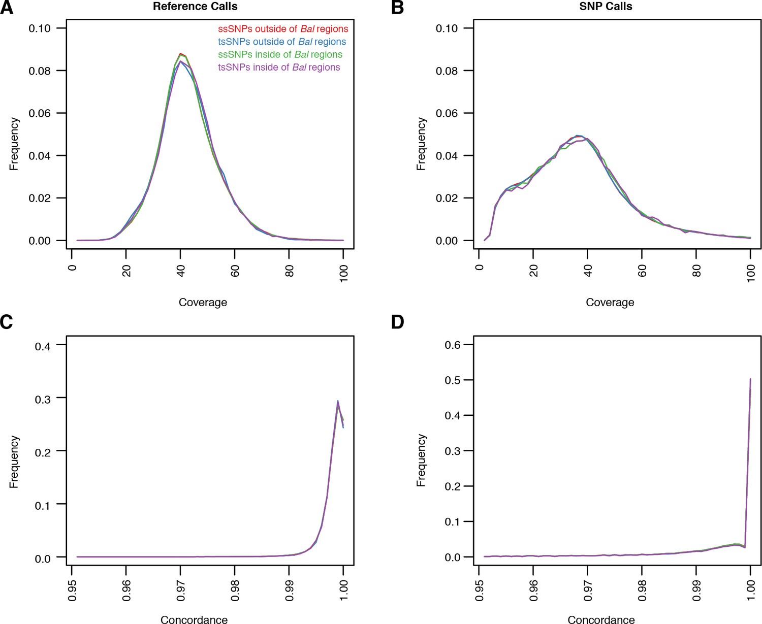
Quality metrics for ssSNPs and tsSNPs in C. rubella.
(A–D) Average coverage and concordance for reference calls (A and C) or non-reference calls (B and D). ssSNPs or tsSNPs outside of regions with significant evidence for balancing selection (red and blue) or inside of these regions (green and purple). Concordance describes the fraction of reads covering a position that supports a particular allele. For example a heterozygous site might have A in 50% of the reads and T in 50% of the reads. The concordance at this site would be 0.5. We show this statistic because our SNP calling method favors homozygous calls in the selfing lineages. If we are missing some heterozygous sites, this would be revealed in the concordance values.
Figure 4—figure supplement 2
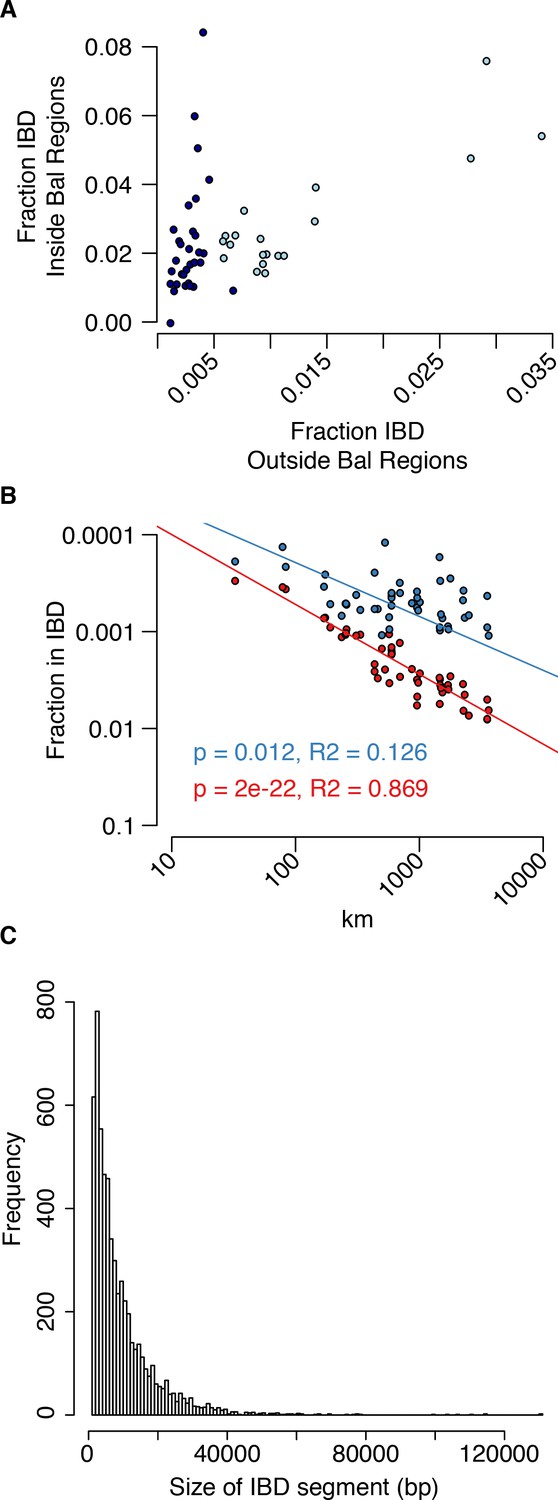
Analysis of IBS in balanced regions and genome-wide.
(A) The relationship between genome-wide and balanced region IBS. Dark blue, west population accessions, Light blue, east population accessions. (B) The decay of IBS genome-wide (red) and within balanced regions (blue) as a function of distance from the centre of C. grandiflora’s range. (C) The genome-wide distribution of IBD segment lengths.
Figure 5 with 2 supplements
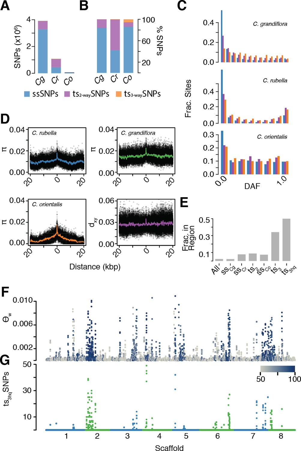
The signal of ancient balancing selection.
(A) Absolute number and (B) fraction of ssSNPs (blue), ts2-waySNPs (purple), and ts3-waySNPs (orange) for Capsella. Only sites accessible to read mapping in all three species were considered. (C) Derived allele frequency (using A. lyrata and A. thaliana as outgroup) of ssSNPs (blue), ts2-waySNPs (purple) and ts3-waySNPs (orange). (D) Pairwise diversity (π) as a function of distance from a ts3-waySNP in C. grandiflora, C. rubella, and C. orientalis. Bottom right, Divergence between the C. rubella/C.grandiflora and C. orientalis lineages as a function of distance from a ts3-waySNP. Black dots, means over all sites at a particular distance, and coloured lines, means over bins of 50 bp. (E) Enrichment of ts3-waySNPs and ts3-wayhqSNPs in candidate balanced regions from the C. rubella/C. grandiflora comparison. (F) Watterson’s estimator (Θw) of genetic diversity in C. orientalis, in 20 kb windows. Grey-to-blue scale indicates the genome-wide percentile of the same window for Θw) in C. rubella. (G) ts3hqSNP number in each window.
-
Figure 5—source data 1
Three species diversity and divergence.
The numbers 1–4 indicate the folddegeneracy of the codon for CDS sites.
- https://doi.org/10.7554/eLife.43606.030
Figure 5—figure supplement 1
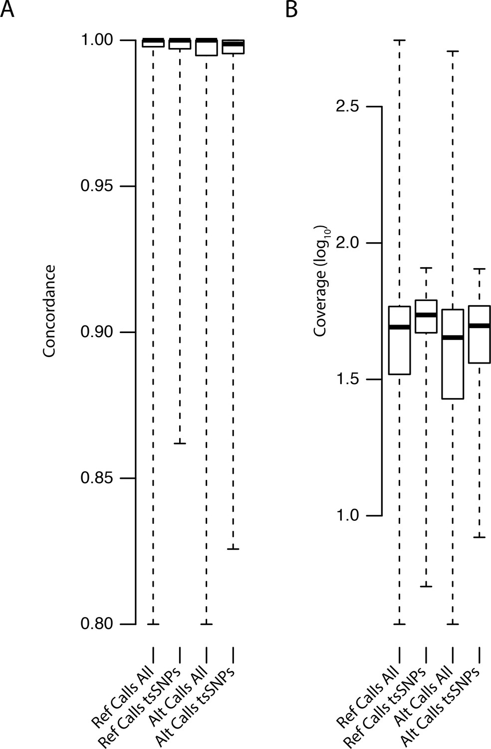
Distributions of concordance and coverage values for different SNP classes in C. orientalis.
https://doi.org/10.7554/eLife.43606.028
Figure 5—figure supplement 2

tr3-wayhqSNPs MAF.
MAF of ssSNPs (blue), ts2-waySNPs (purple), and ts3-waySNPs (orange) in each species (top: C. grandiflora, middle: C. rubella, bottom: C. orientalis).
Figure 6 with 3 supplements

Evidence for long-term balancing selection at MLO2.
(A) Diagram of MLO2 protein in the cell membrane. Blue ovals, transmembrane domains. Top is the extracellular space. Orange dots represent amino acid differences between proteins encoded by haplogroups A and B. (B) Haplogroup identification with reference based SNP calls. Circles represent ts3-wayhqSNPs and colours represent the reference (green) and alternative (blue) SNP calls. Numbers indicate haplotype frequencies in each species. (C) Top: A diagram of the MLO2 region on scaffold 1. Grey boxes represent coding regions. Empty circles show the positions of the seven initially identified ts3-wayhqSNPs shown in (B). MLO2b gene is drawn based on the reference annotation, but alignment with orthologous genes suggested a misannotation of the last splice site acceptor leading to truncation of the annotated gene. For final alignments, the corrected annotation was used. Middle: Average read coverage by haplogroup and species (blue is C. rubella and orange is C. orientalis). Region of poor coverage in haplogroup B is highlighted with a black bar. The green and yellow bars below the coverage plots highlight the de novo assembled region and the windows from which the neighbour-joining trees were built (excluding indels, each window is 1 kb). The blue and orange circles on the tree indicate samples from each species. Black scale indicates substitutions in trees.
Figure 6—figure supplement 1

Sliding windows of allelic divergence and positions of tsSNPs.
Divergence between haplotype A and B within species, or between the same haplotype across species at the MLO2 locus. Circles indicate positions of SNPs by class.
Figure 6—figure supplement 2
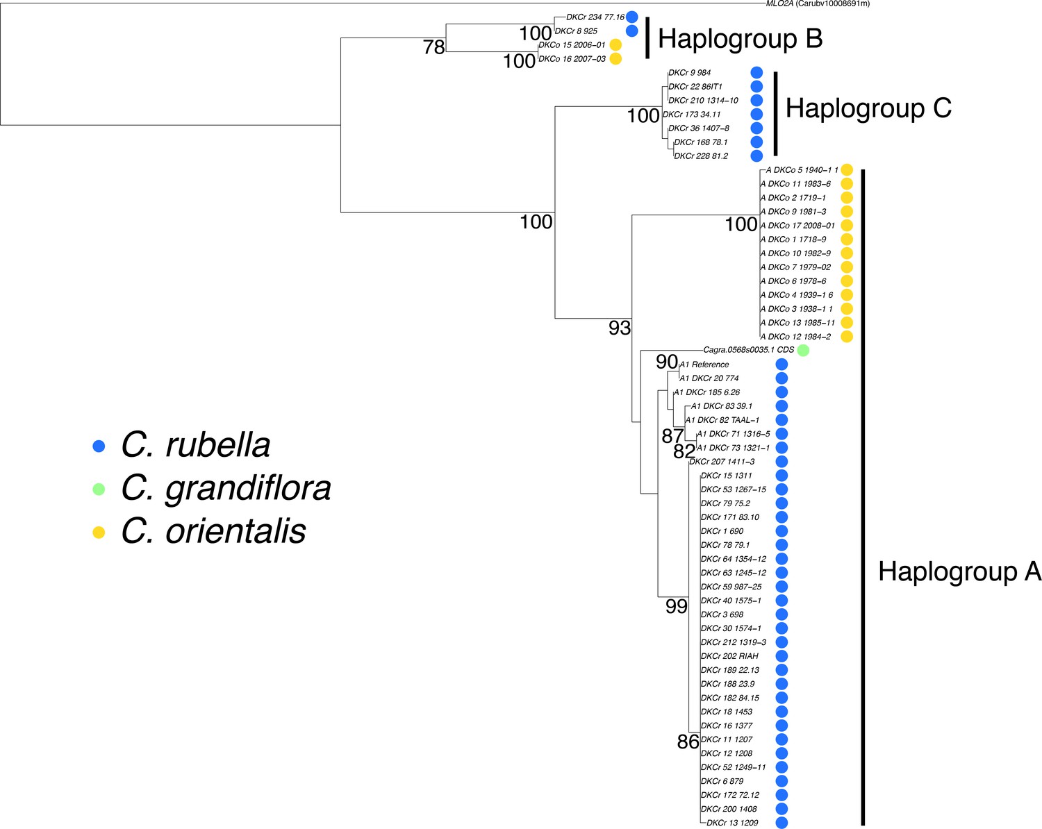
Phylogenetic analysis of the MLO2 CDS.
A maximum likelihood phylogeny depicting the relationship between MLO2B haplogroups. MLO2A was used to set the root of the tree. Bootstrap values for branches supported more than 75% of the time are shown.
Figure 6—figure supplement 3
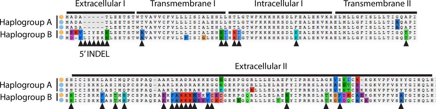
Alignment of amino acid sequences at the MLO2 N-terminus.
Examples of alleles from each haplogroup in each species are shown. Triangles show fixed amino acid substitutions between the two alleles. The inferred domain structure is shown above the alignments.
Additional files
-
Supplementary file 1
GO enrichment analysis of tsSNPs.
- https://doi.org/10.7554/eLife.43606.035
-
Supplementary file 2
GO enrichment for tr3-waySNPs.
- https://doi.org/10.7554/eLife.43606.036
-
Supplementary file 3
List of well covered genes for targeted analysis of potential balancing selection.
- https://doi.org/10.7554/eLife.43606.037
-
Supplementary file 4
Pericentromeric or repeat dense genomic regions filtered in genome scans.
- https://doi.org/10.7554/eLife.43606.038
-
Supplementary file 5
Annotation hierarchies for SNPs with multiple annotations.
- https://doi.org/10.7554/eLife.43606.039
-
Supplementary file 6
List of A. thaliana NLR genes used for ortholog identification.
- https://doi.org/10.7554/eLife.43606.040
-
Transparent reporting form
- https://doi.org/10.7554/eLife.43606.041
Download links
A two-part list of links to download the article, or parts of the article, in various formats.
Downloads (link to download the article as PDF)
Open citations (links to open the citations from this article in various online reference manager services)
Cite this article (links to download the citations from this article in formats compatible with various reference manager tools)
Long-term balancing selection drives evolution of immunity genes in Capsella
eLife 8:e43606.
https://doi.org/10.7554/eLife.43606


