Complementary networks of cortical somatostatin interneurons enforce layer specific control
- Alexander Naka

- Julia Veit
- Ben Shababo
- Rebecca K Chance
- Davide Risso
- David Stafford
- Benjamin Snyder
- Andrew Egladyous
- Desiree Chu
- Savitha Sridharan
- Daniel P Mossing
- Liam Paninski
- John Ngai
- Hillel Adesnik
- University of California, Berkley, United States
- University of Padova, Italy
- Weill Cornell Medicine, United States
- Columbia University, United States
Figures
Figure 1 with 4 supplements
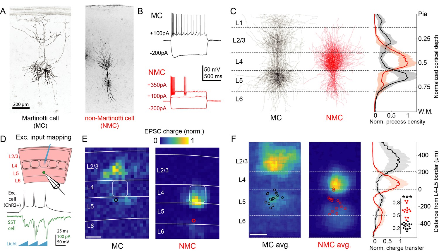
Optogenetic circuit mapping reveals complementary synaptic input patterns to two subtypes of L5 SST cells.
(A) Confocal images of dye filled neurons revealing two morphological phenotypes of L5 SST cells. Left: an L5 GIN cell. Right: an L5 × 94 cell. Scale bar: 200 µm. (B) Example traces during current step injections from an L5 GIN cell (black) and an L5 × 94 cell (red). (C) Left: Overlaid morphological reconstructions of L5 GIN/MC cells (black, n = 14) and L5 × 94/NMCs (red, n = 10) showing differences in laminar distribution of neurites. Right: Normalized neurite density versus cortical depth for L5 GIN (black) and L5 × 94 cells (red). Data are represented as mean ±C.I. Note that these reconstructions do not distinguish between axon and dendrite; for detailed morphological analysis of these cells, see (Ma et al., 2006) (D) Schematic of experimental configuration. A digital micromirror device was used to focally photo-stimulate excitatory cells in different regions of the slice in order to map the spatial profile of excitatory inputs to GFP +L5 MCs (Emx1-Cre; GIN) or GFP +L5 NMCs (Emx1-Cre; X94). (E) Example heat maps of median EPSC charge transfer evoked at each stimulus site for example L5 SST cells. Left: An L5 MC that received inputs from L5 and L2/3. Right: An L5 NMC that received inputs from L4 and the L5/6 border. Soma locations are indicated by red/black bordered white dot). Scale bar: 200 µm. (F) Left: Grand averages of input maps reveal cell-type specific patterns of laminar input. Soma locations are indicated as above. Right: Normalized charge transfer versus distance from L4-L5 border for MC (black) and NMC (red) populations. Scale bar: 200 µm. Inset: Swarm plots showing the proportion of total evoked charge transfer in each map that originated from sites in L4 +L6, that is [L4+L6] / [L2/3+L4+L5+L6] for the MC (black; median, 27%; range, 13–36%) and NMC (red; median, 62%; range, 38–84%) populations. Proportions were significantly different between L5 MCs and L5 NMCs (25 ± 3% in n = 15 MCs versus 62 ± 7% in n = 14 NMCs, mean ±C.I.; p=6.5 · 10−10; two-sample t-test). See also Figure 1—figure supplement 1–4.
Figure 1—figure supplement 1
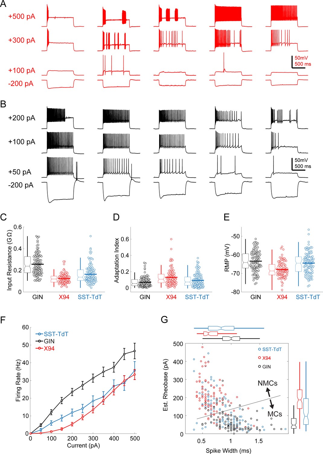
Intrinsic properties of L5 SST cells.
(A) Example traces showing diverse spiking responses of L5 × 94 cells during current injection. (B) As in A, but for L5 GIN cells. Note that less current is being injected due to the greater input resistance of these cells. (C) Swarm and box-and-whisker plots of input resistance for L5 GIN cells (black), L5 × 94 cells (red), and L5 SST-TdT cells (gray). Thick horizontal line indicates distribution mean. (D,E) As in C, but for spike frequency adaptation index and resting membrane potential. (F) FI curves from L5 cells recorded in the SST-TdT line (gray), GIN line (black), or X94 line (red). (G) Scatter plot showing estimated rheobase and median spike width for L5 GIN cells (black), L5 × 94 cells (red), and L5 SST-TdT cells (gray). Box and whisker plots summarizing population statistics for these variables are in the margins. The blue line indicates the decision boundary for a linear support vector machine trained to classify L5 GIN cells and L5 × 94 cells based on these two variables; this classifier was in turn used to classify SST-TdT cells as putative NMCs or MCs.
Figure 1—figure supplement 2
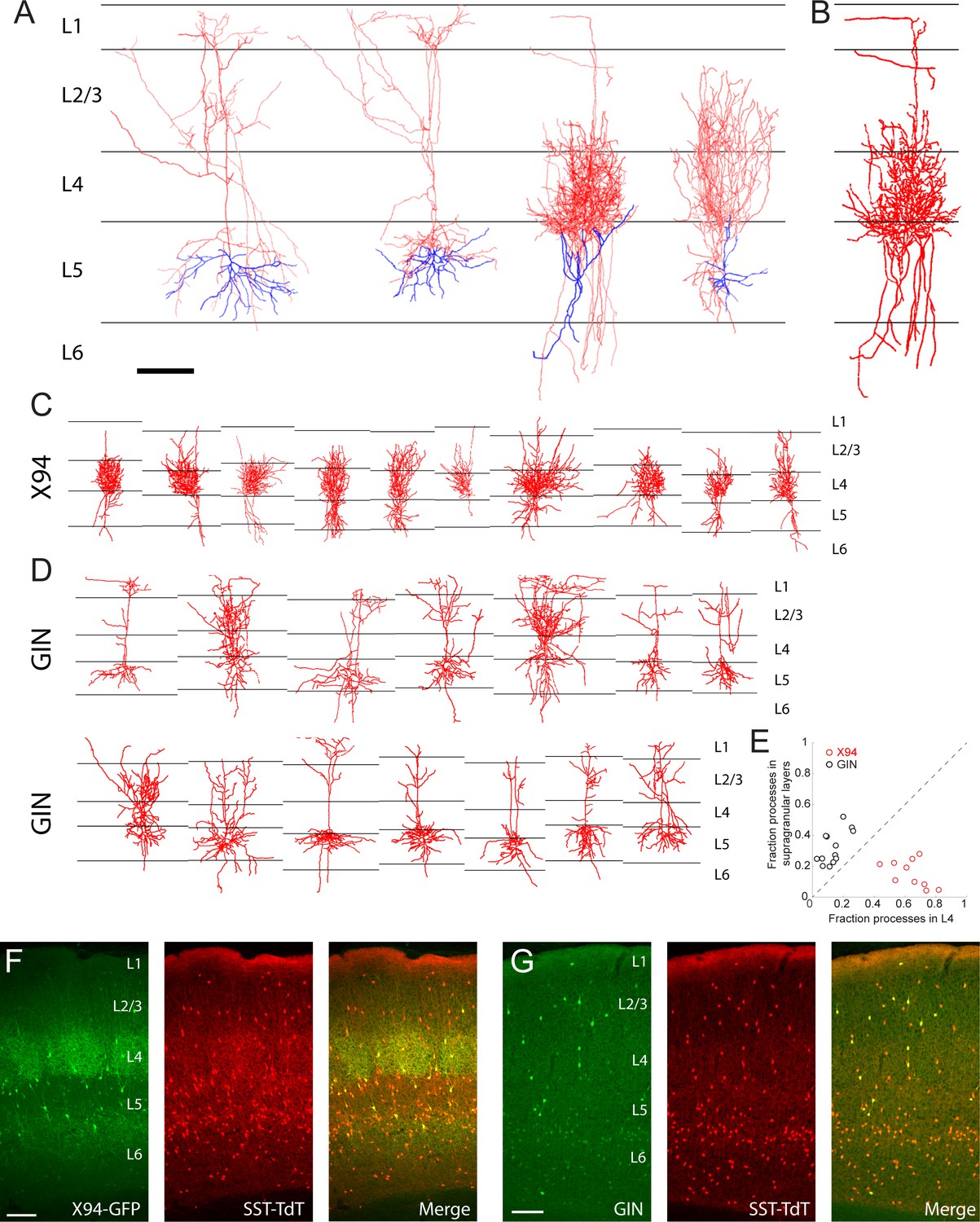
Morphological reconstruction of L5 SST cells.
(A) Examples of biocytin reconstructions done manually at high magnification of two L5 MCs (left two) and two L5 NMCs (right two) showing axonal (red) and dendritic (blue) morphology. Scale bar 150 µm. (B) An example of a semi-automated reconstruction done at 10x magnification of an L5 NMC (compare to the third reconstruction in A). (C) Semi-automated reconstructions of L5 × 94 cells (D) As in C, but for L5 GIN cells. (E) Comparison of neurite density of L5 GIN cells and L5 × 94 cells in L4 versus the supragranular layers. (F) Coronal section of barrel cortex in an X94-GFP; SST-TdT mouse. TdTomato fluorescence can be seen in all layers, with a dense band in L1 from the axons of MCs. Dense axonal arborization of X94-GFP cells is visible in L4, and upper L6 to a lesser extent, but not in L1. (G) As in F, but for a GIN; SST-TdT mouse.
Figure 1—figure supplement 3
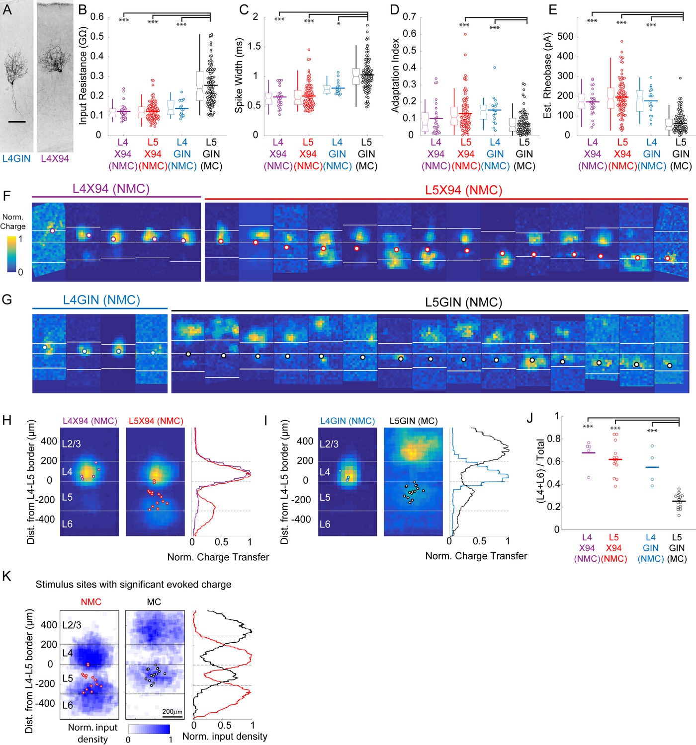
Comparison of intrinsic properties and excitatory inputs for L4 and L5 SST cells.
(A) Biocytin fills of an L4 GIN cell (left) and an L4 × 94 cell (right), both exhibiting non-Martinotti morphology. (B) Input resistances for L4 × 94, L5 × 94, L4 GIN, and L5 GIN populations. Data are displayed as swarm plots, accompanied by Tukey box plots. The thick horizontal bar within the swarm indicates population mean. The L4 × 94, L4 GIN, and L5 × 94 populations have significantly lower input resistances than the L5 GIN population (L4 × 94, p=3.8 · 10−9; L5 × 94, p=3.8 · 10−9; L4 GIN, p=3.8 · 10−5; Wilcoxon rank-sum test versus L5 GIN population). (C) As in B, but for spike width. The L4 × 94, L4 GIN, and L5 × 94 populations have significantly shorter spike widths than the L5 GIN population (L4 × 94, p=4.0 · 10−9; L5 × 94, p=3.8 · 10−9; L4 GIN, p=0.029; Wilcoxon rank-sum test versus L5 GIN population). (D) As in B, but for adaptation index score. The L4 GIN and L5 × 94 populations have significantly shorter spike widths than the L5 GIN population (L5 × 94, p=1.5 · 10−6; L4 GIN, p=1.4 · 10−4; Wilcoxon rank-sum test) but the L4 × 94 was not significantly different. (E) As in B, but for estimated rheobase. The L4 × 94, L4 GIN, and L5 × 94 populations have significantly shorter spike widths than the L5 GIN population (L4 × 94, p=7.2 · 10−9; L5 × 94, p=3.8 · 10−9; L4 GIN, p=6.4 · 10−7; Wilcoxon rank-sum test versus L5 GIN population). (F) All excitatory input maps for X94 cells in L4 (left, orange) and L5 (right, red). Bordered white dots indicate the location of the recorded soma. (G). As in F, but for GIN cells in L4 (gray) and L5 (black). (H) Average maps for L4 and L5 NMCs. Both groups receive strong input from L4. L5 NMCs receive stronger inputs on average from the infragranular layers, though there was no significant difference between these groups nor a significant correlation of the depth of the recorded cell with the relative amount of input received from the deeper layers. (I) As in H, but for GIN cells. L4 GIN cells (NMCs) receive inputs primarily from L4 (similar to X94 cells) and are very different from L5 GIN cells (MCs). (J) L5 GIN MCs received a significantly smaller proportion of excitatory charge transfer originating from L4 and L6 than other cell types (L4 × 94, p=7.2 · 10−9; L5 × 94, p=3.8 · 10−9; L4 GIN, p=6.4 · 10−7; Wilcoxon rank-sum test versus L5 GIN population). (K) Averages of binary input maps for L5 NMCs and L5 MCs. Binary input maps were generated by testing whether evoked charge was statistically significant at individual stimulation sites. For each site, a permutation test was performed comparing evoked charge to a null distribution of charge generated by resampling from recording periods without stimulation. Maps were then thresholded for significance following a Bonferroni correction for multiple comparisons. Single asterisk indicates p<0.05, three asterisks indicates p<0.001.
Figure 1—figure supplement 4
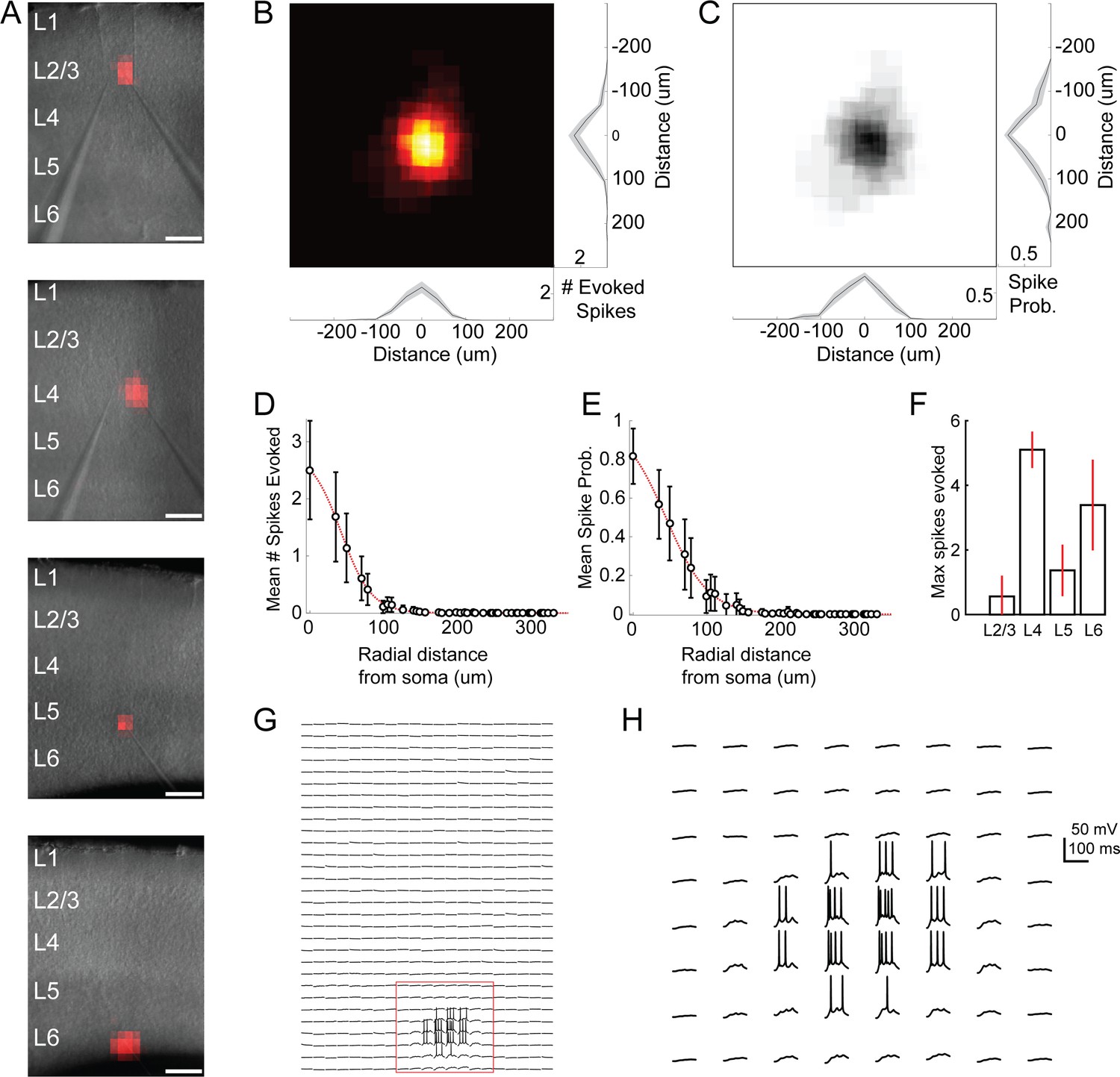
Excitation profiles of ChR2 +cells in Emx-Cre DMD-based one photon optogenetic mapping experiments.
(A) Example spiking heatmaps recorded from cells in L2-6, overlaid on infrared images of slices. Scale bar indicates 175 µm. (B) Average map of # of evoked spikes per trial in n = 20 ChR2 +cells. Maps are centered on the somata of recorded cells. (C) As in B, but for probability of evoking at least one spike per trial. (D) Average number of spikes evoked as a function of radial distance from ChR2 +cell soma. (E) As in D, but for probability of evoking at least one spike. (F) Max number of spikes evoked per trial at the most effective stimulus site (e.g. over the soma) for ChR2 +cells in different layers. Errorbars denote 95% C.I. (G) Example traces corresponding to the bottom heatmap in A. Spiking is evoked only during perisomatic photostimulation. (H) Expanded view of red boxed region in F. Bursts of spikes are evoked in a single trial during direct stimulation of the soma.
Figure 2 with 1 supplement
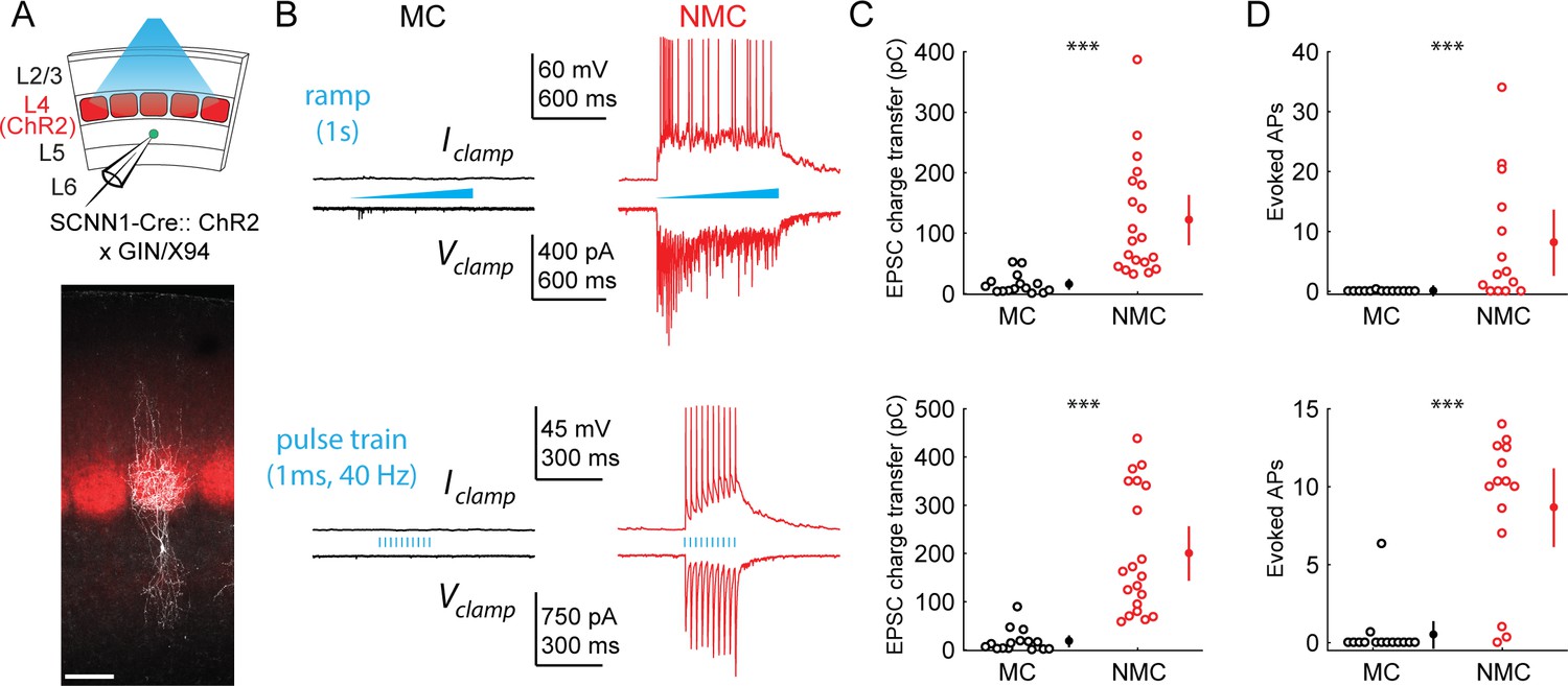
L4 photo-stimulation excites L5 NMCs but not L5 MCs.
(A) Top: Schematic of the experimental configuration. L5 × 94 or GIN cells were recorded during photo-stimulation of L4 excitatory neurons. Bottom: Confocal image of a filled L5 × 94 neuron (white) with ChR2-TdTomato expression (red) visible in L4. Scale bar: 150 µm. (B) Top row: Example traces recorded in the current clamp (upper traces) or voltage clamp (lower traces) configurations during a 1 s ramp photo-stimulation. Bottom row: As above, but for photo-stimulation with a 40 Hz train of ten 1 ms pulses. (C) Quantification of excitatory charge transfer during maximum intensity 1 s ramp stimulation trials. Mean 122 ± 41 pC in n = 20 NMCs versus 15 ± 8 pC in n = 15 MCs; p=3.9 · 10−6, Wilcoxon rank sum test. (D) Quantification of the mean number of evoked action potentials during maximum intensity 1 s ramp stimulation trials. Mean 8.1 ± 5.5 spikes per trial in n = 15 NMCs versus 0.03 ± 0.05 spikes per trial in n = 15 MCs; p=6.6 · 10−4, Wilcoxon rank sum test. (E) As in C, for maximum intensity 40 Hz pulse train stimulation. Mean 200 ± 56 pA in n = 20 NMCs versus 18 ± 12 pA in n = 15 MCs; p=2.8 · 10−6, Wilcoxon rank sum test. (F) As in D, for maximum intensity 40 Hz pulse train stimulation. Mean 8.7 ± 2.4 spikes per trial in n = 15 NMCs versus 0.5 ± 0.9 spikes per trial in n = 15 MCs; p=1.5 · 10−6, Wilcoxon rank sum test. Error bars denote mean ±95% confidence interval. Three asterisks denotes p<0.001.
Figure 2—figure supplement 1
Responses of L4 and L5 SST cells to L4 photo-stimulation.
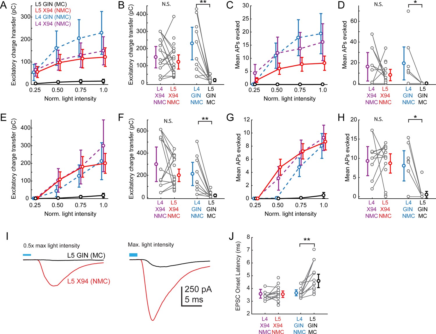
The aim of these experiments was to compare the amount of L4 input received by L5 NMCs and L5 MCs, which required us to perform experiments in two sets of animals (SCNN1-Cre; X94 mice and SCNN1-Cre; GIN mice). Whenever possible while recording from an L5 × 94 (NMC) or L5 GIN (MC), we also recorded simultaneously from an L4 NMC, exploiting the fact that in L4, NMCs are labeled in both the X94 and the GIN lines. This configuration acts as a control for possible variability (e.g. in opsin expression, slice health) that is bound to occur to some extent between different slices and animals. (A) Dose response profile of excitatory charge transfer evoked during 1 s ramp stimulation of L4 for X94 cells in L4 (purple) and L5 (red) and for GIN cells in L4 (blue) and L5 (black). To assess differences between groups, we fit a linear mixed-effects model with fixed effects parameters for the slope of the stimulus-response function and random effects slope parameters for each slice and cell recorded, along with a single intercept term. The L5 GIN cell group had a significantly lower fixed effects slope coefficient than the L5 × 94 (p=2.1 · 10−5), L4 × 94 (p=3.1 · 10−5), and L4 GIN groups (p=2.0 · 10−9). (B) Mean excitatory charge transfer evoked during maximum intensity 1 s ramp stimulation of L4. Gray lines indicate pairs of cells recorded in the same slice. Charge transfer was not significantly different between L4 × 94 cells and L5 × 94 cells on a pairwise basis (169.1 ± 91.5 pC versus 118.7 ± 44.0 pC; p=0.10, paired t-test), but was significantly different between L4 GIN cells and L5 GIN cells (229.4 ± 95.3 pC versus 15.2 ± 8.4 pC; p=0.002, paired t-test). (C,D) As in A,B, but for mean number of action potentials evoked in L5 SST cells recorded in current clamp during 1 s ramp photo-stimulation. F-tests on coefficients of a linear mixed-model indicated that the L5 GIN cell group had a significantly lower fixed effects slope coefficient than the L5 × 94 (p=0.03), L4 × 94 (p=1.0 · 10−3), and L4 GIN groups (p=1.7 · 10−4). The mean number of spikes evoked was not significantly different between L4 × 94 cells and L5 × 94 cells on a pairwise basis (20.4 ± 23.7 spikes versus 9.0 ± 6.0 spikes; p=0.14, paired t-test), but was significantly different between L4 GIN cells and L5 GIN cells (19.4 ± 16.0 spikes versus 0.03 ± 0.05 spikes; p=0.034, paired t-test). (E,F). As in A,B, but for excitatory charge transfer in L5 SST cells recorded in voltage clamp during a train of ten 1 ms pulses at 40 Hz. F-tests on coefficients of a linear mixed-model indicated that the L5 GIN cell group had a significantly lower fixed effects slope coefficient than the L5 × 94 (p=1.2 · 10−6), L4 × 94 (p=3.5 · 10−9), and L4 GIN groups (p=5.2 · 10−16). Charge transfer was not significantly different between L4 × 94 cells and L5 × 94 cells on a pairwise basis (309.1 ± 220.6 pC versus 191.5 ± 58.8 pC; p=0.055, paired t-test), but was significantly different between L4 GIN cells and L5 GIN cells (212.2 ± 104.7 pC versus 18.0 ± 12.2 pC; p=0.002, paired t-test). (G,H). As in A,B, but for mean number of action potentials evoked in L5 SST cells recorded in current clamp during a train of ten 1 ms pulses at 40 Hz. F-tests on coefficients of a linear mixed-model indicated that the L5 GIN cell group had a significantly lower fixed effects slope coefficient than the L5 × 94 (p=1.2 · 10−6), L4 × 94 (p=5.3 · 10−9), and L4 GIN groups (p=2.2 · 10−14). The mean number of spikes evoked was not significantly different between L4 × 94 cells and L5 × 94 cells on a pairwise basis (9.8 ± 6.2 spikes versus 8.6 ± 2.6 spikes; p=0.56, paired t-test), but was significantly different between L4 GIN cells and L5 GIN cells (8.0 ± 3.9 spikes versus 0.5 ± 0.9 spikes; p=0.0068, paired t-test). (I) Plots of the grand average EPSC evoked at mild intensity (top; 0.625 mW·mm (Harris and Shepherd, 2015)) pulse and maximum intensity stimulation (bottom; 1.25 mW·mm (Harris and Shepherd, 2015)) of L4 for L5 MCs (black) and L5 NMCs (red). Low intensity stimulation produced robust EPSCs in L5 NMCs but not L5 MCs. High intensity stimulation was able to evoke EPSCs L5 MCs but with a delayed onset. (J) Plot of average EPSC onset latency in response to maximum intensity pulse stimulation of L4 (as seen in bottom panel of I) in different SST cell populations. Gray dots indicate individual cells in each group; cells connected by gray lines indicate neurons recorded in the same preparation (usually simultaneously). EPSC onset latency is uniformly longer for L5 MCs compared to paired L4 NMCs. Errorbars indicate mean ±95% confidence interval.
Figure 3 with 2 supplements

two photon optogenetic circuit mapping reveals that L4 and L5 PCs are inhibited by separate populations of L5 SST cells.
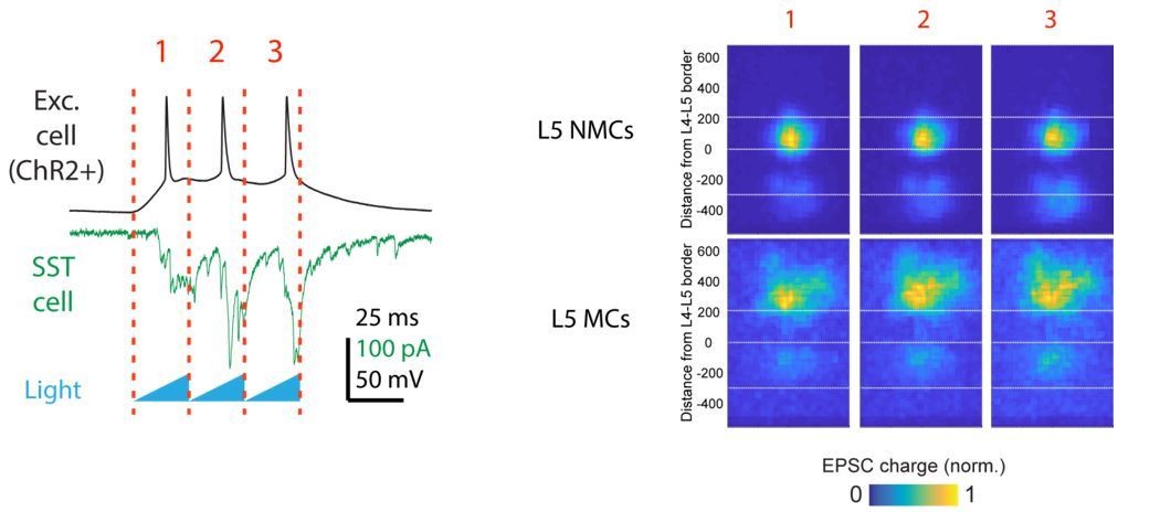
(A) Schematic of the experimental configuration. IPSCs are recorded from a pair of PCs (either an L4/L5 pair or an L5/L5 pair) while SST cells expressing soma-targeted ChrimsonR-mRuby2 are focally activated using 2P photo-stimulation and computer generated holography. (B) Left: post-hoc confocal image showing SST cells expressing soma-targeted-ChrimsonR-mRuby2 (red) and biocytin fills of recorded PCs in L4 and L5 (white) at 10x magnification. Right: Confocal image at 20x magnification showing the grid of photo-stimulated target locations. Both images are max z-projections over 100 μm. (C) Spatial photo-excitation profile of a soma-targeted-ChrimsonR-mRuby2 expressing SST cell. Whole cell current-clamp recordings from this cell showing multiple trials of photo-stimulation at a 4 × 4 subsection of the photo-stimulation grid with 20 μm spacing between stimulation locations. The SST cell is recruited to spike only at a small number of stimulation sites, but does so reliably and with low jitter across trials at these sites. (D) Example traces showing IPSCs recorded from an L4 PC during SST photo-stimulation at a single site (corresponding to black boxed square in E) over multiple trials. Dots above each trace indicate the onset time of detected IPSCs (p=0.0003, Poisson detection). (E) Example overlay of maps showing the mean number of IPSCs at detected input locations during photo-stimulation for a simultaneously recorded L4 PC-L5 PC pair. Bubble size indicates the mean number of IPSCs evoked (deviation from background rate) per trial. (F) As in E, but for an L5 PC-L5 PC pair. (G) Example traces illustrating method for detection of common SST-mediated inputs to pairs of simultaneously recorded PCs. Left: IPSC traces at a single site recorded simultaneously in two PCs (each PC is indicated by black or grey traces) and corresponding detected IPSCs. IPSCs with synchronous onset occur in many trials, despite the trial-to-trial jitter in IPSC onset, suggesting that a SST cell which diverges onto both recorded PCs is being stimulated at this site (p=0.0005, synchrony jitter test). Right: IPSC traces from a different site. Evoked IPSCs are observed in both cells, but the lack of synchronicity suggests they arise from separate, neighboring SST cells (p=0.4). Dots above each trace indicate the estimated onset time of detected IPSCs. (H) Probability of detecting common SST input per photo-stimulated site for pairs consisting of L4 PCs and L5 PCs versus pairs consisting of two L5 PCs. No common input locations were detected in n = 10 L4-L5 pairs versus 13.7 ± 5.1% of all input locations locations stimulated in n = 10 L5-L5 pairs; p=1.1 · 10–3, Wilcoxon rank sum test Data are summarized by mean ±S.E.M. (I) Schematic of main result for SST outputting mapping. Individual L5 SST cells form inhibitory connections onto L4 PCs and or L5 PCs but not both.
Figure 3—figure supplement 1
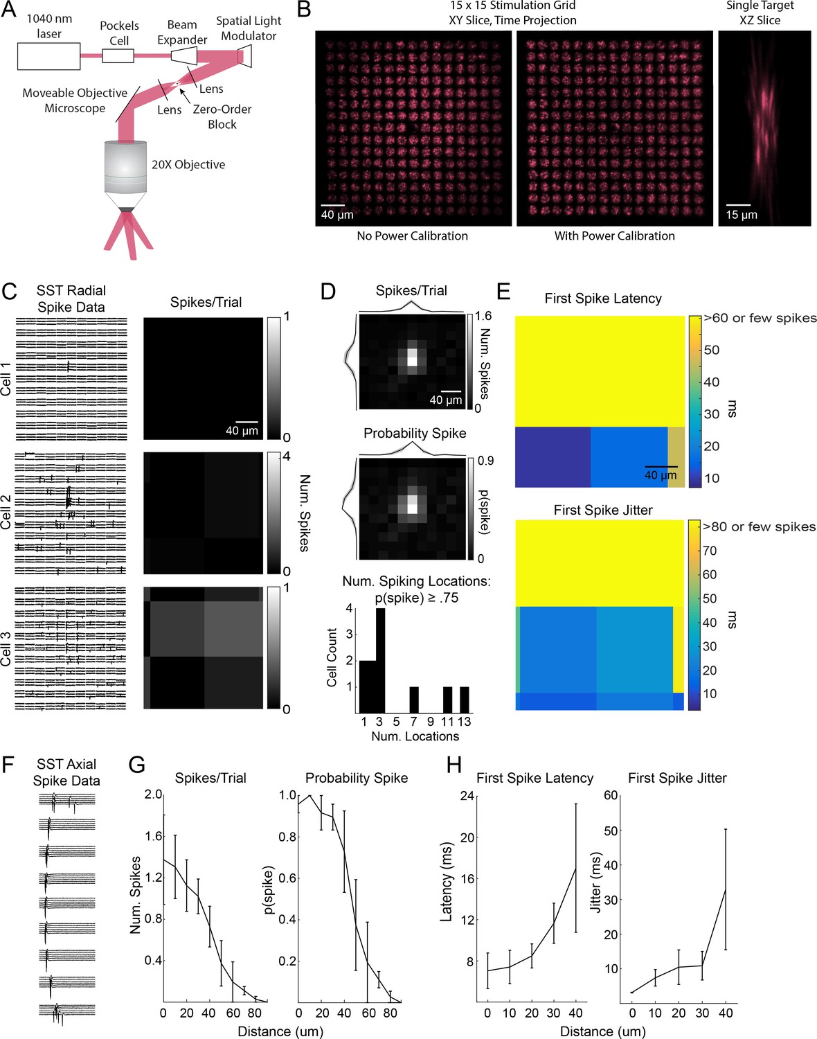
Excitation profiles of st-ChrimsonR-expressing SST cells in multiphoton holographic SST-Cre mapping experiments.
(A) Schematic of the CGH-based stimulation microscope. (B) Imaging stimulation holograms with two-photon induced fluorescence in a thin fluorescent slide. Left: Time projection of a stimulation sequence covering a 15 × 15 grid of targets at 20 μm spacing before power calibration. Middle: As in Left but with power calibration. Left: XZ slice of a single target. Note that excitation is confined to a small volume and that power calibration results in more uniform excitation radially. The decrease in fluorescence in the middle of the two stimulation grids is due to the zero-order block. (C) Example plots of the lateral resolution of photo-stimulation. Left column: Raw cell-attached data of light-evoked spiking for example SST cells. Right column: average number of spikes evoked per trial at each location. Locations are 20 µm apart as in mapping experiments. (D) Radial spike count statistics. Top: Average map of the number of evoked spikes per trial in st-ChrimsonR +cells (n = 11). Maps are centered on the somata of recorded cells. Middle: As in top, but for probability of evoking at least one spike per trial. Bottom: Histogram of number of locations per cell which evoked a spike at least 75% of the trials. (E) Radial spike timing statistics. Top: Average first spike latency for st-ChrimsonR +cells (n = 11). Yellow indicates that the average was >60 ms or that too few spikes were observed across cells at those locations to obtain a good estimate. Bottom: Average first spike jitter, computed as the full-width half-maximum of the first spike times. Yellow indicates a jitter of greater than 80 msec or that too few spikes were observed across cells at those locations. (F) Data from an example cell as the hologram is moved axially. Distance between locations is 10 µm. (G) Axial spike count statistics. Left: Average number of evoked spikes as a function of axial distance for st-ChrimsonR +cells (n = 4). Right: As in left, but for the probability of at least one spike per trial. (H) Axial spike timing statistics. Left: Average first spike latency as a function of axial distance (n = 4 cells). Right: First spike jitter as a function of axial distance for st-ChrimsonR +cells (n = 3).
Figure 3—figure supplement 2
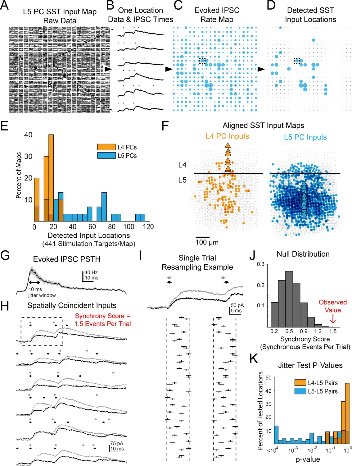
Data processing and additional results for multiphoton SST output mapping.
(A) Example of raw data a single map onto a L5 PC. Dashed box shows location for which data is shown in B. (B) Example of Bayesian PSC detection on all six trials from a single location from the map in A. (C) A map showing the evoked IPSC rates at each location for the map from A. Dashed box shows location of data from B. (D) As in C except only locations which pass FDR detection are shown. (E) Histograms showing the number of locations with evoked IPSCs in each map recorded for both L4 and L5 PCs. (F) Overall spatial input distributions for SST cells in L5 to both L4 PCs (left, n = 10) and L5 PCs (right, n = 28). Maps are aligned vertically to the L4-L5 border and horizontally to the PC soma. For this representation all inputs are plotted with the same size circle. (G). PSTH of IPSC times aggregated from all locations with detected evoked IPSC rates. A 10 ms duration which matches the jitter duration for temporal synchrony is marked for comparison. (H) As in B except showing data and IPSC detection for two simultaneously recorded L5 PCs. The synchrony score for this location is 1.5 events/trial. Dashed box shows data used for I. (I) Example of 20 resamplings of the events during the analysis window for the first trial shown in H. Vertical dashed lines show discrete event jittering windows. Horizontal lines on each event span 2 ms such that if the lines from two events overlap then they would be counted as synchronous. (J) Null distribution of synchrony score from event time series resampling of the data in H. The observed value is from the far right extreme of the distribution. (K) Histograms of p-values for all spatially overlapping locations for all pairs from jitter synchrony tests.
Figure 4 with 3 supplements

MCs and NMCs exhibit different patterns of monosynaptic connectivity with L4 and L5 PCs.
(A) Paired recordings of L4 PCs (orange) and L5 NMCs/MCs (red/black).). Left: schematic of the tested circuit. Middle: example traces of evoked spikes in a L4 PC (orange) and the excitatory synaptic current in a L5 NMC (red). Right: example traces of evoked IPSPs in a L4 PC (orange) in response to a single action potential in a L5 NMC (red). (B) Bar graph summarizing translaminar connection rates between L4 PCs and L5 MCs (black bars) and L4 PCs and L5 NMCs (red bars). p<10−6 for L4PC→L5MC (n = 95 connections tested onto 39 MCs) versus L4 PC→L5 NMC connection rate (n = 72 connections tested onto 51 NMCs); p=2·10−6 for L5MC→L4PC (n = 68 connections tested from 35 MCs) versus L5 NMC →L4PC connection rate (n = 67 connections tested from 51 NMCs); Monte Carlo permutation test. (C) As in A, but intralaminar pairs between L5 MCs/NMCs and L5 PCs (blue). (D) As in B, but for intralaminar connections with L5 PCs. p=0.020 for L5 PC→L5 MC (n = 29 connections tested onto 20 MCs) versus L5 PC→L5 NMC connection rate (n = 60 connections tested onto 35 NMCs); p<10−6 for L5 MC→L5 PC (n = 46 connections tested from 30 MCs) versus L5 NMC →L5 PC connection rate (n = 65 connections tested from 37 NMCs); Monte Carlo permutation test. See also Figure 4—figure supplement 1–3 and Table 1.
Figure 4—figure supplement 1
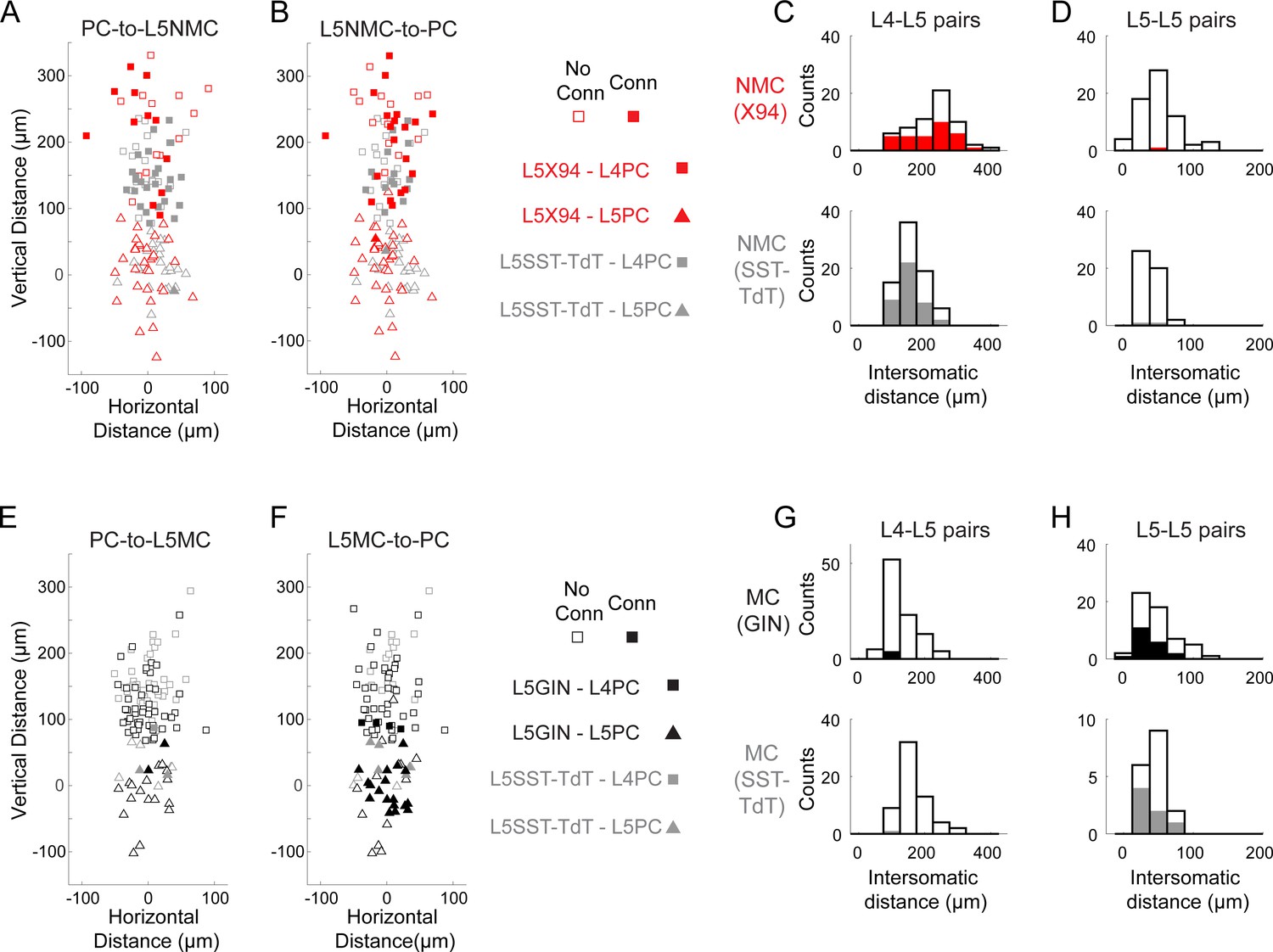
Distances of connections tested in paired recordings.
(A) Scatterplot showing the relative distances between pairs tested for monosynaptic excitatory connections from L4 and L5 PCs onto L5 NMCs. Squares represent L5 NMC - L4 PC pairs; triangles represent L5 NMC - L5 PC pairs. Filled markers indicate that a connection was observed; open markers indicate no connection was observed. Red symbols indicate pairs tested in X94 mice; gray symbols indicate pairs tested in SST-TdT mice where the L5 NMC was identified electrophysiologically. The origin represents the position of the L5 NMC soma (note that these were located at variable distances from the L4-L5 border). (B) As in A, but for monosynaptic inhibitory connections from L5 NMCs onto L4 and L5 PCs. (C) Histogram showing the distribution of intersomatic distances between pairs of L5 NMCs and L4 PCs. Empty bars indicate the number of pairs tested per binned distance; filled bars indicate the number of positive connections (unidirectional in either direction or bidirectional) detected at that bin. Top: pairs in X94 mice. Bottom: pairs in SST-TdT mice. (D) As in C, but for pairs of L5 NMCs and L5 PCs. (E–H) As in A-D, but for pairs of L5 MCs and L4/L5 PCs. Other than the layer-specific connectivity biases of MCs and NMCs, we did not observe any significant relationship between intersomatic distance (vertical, horizontal, or Euclidean) and connection probability.
Figure 4—figure supplement 2
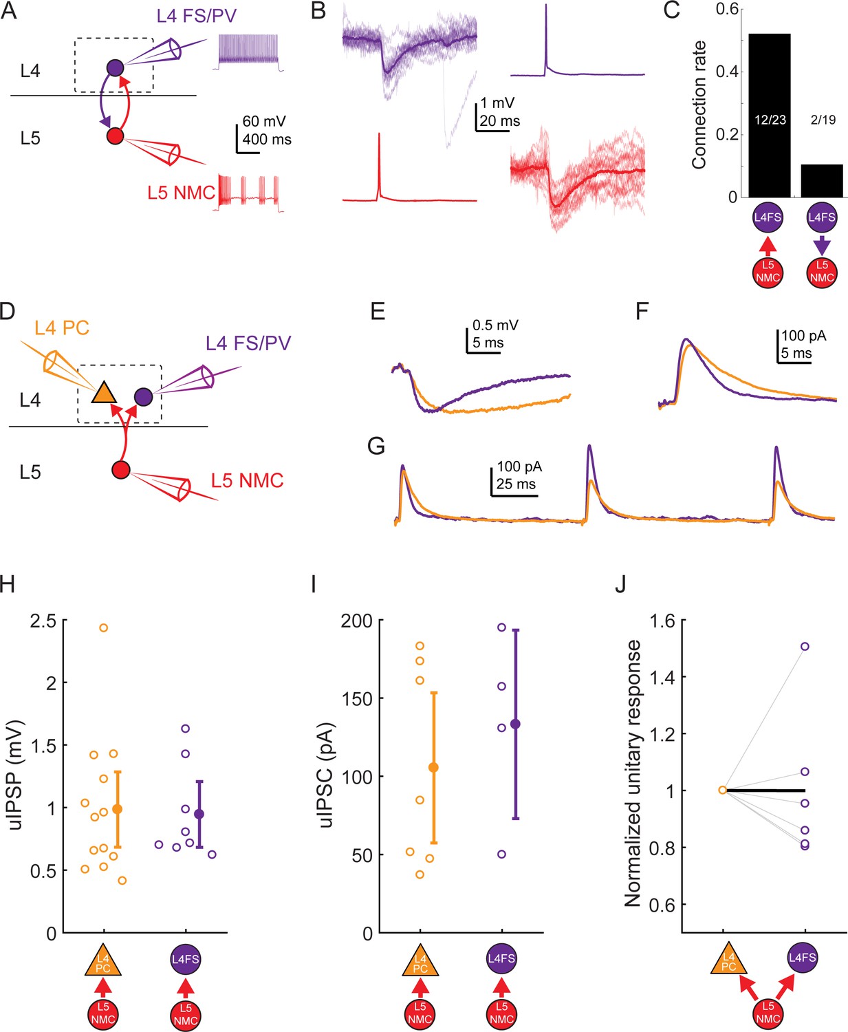
L5 NMC connectivity onto L4 FS cells.
(A) Schematic of paired recordings between L4 FS/PV cells (purple) and L5 NMCs. Inset: example spiking in response to depolarizing current injection. (B) Monosynaptic IPSPs could be observed in L4 FS cells in response to single spikes in L5 NMCs (left) and vice versa (right) (C) Bar graph showing connection rates for L5 NMC - L4FS pairs. Connections from L5 NMCs onto L4 FS cells were observed frequently, whereas connections from L4 FS cells onto L5 NMCs occurred rarely. (D) In some experiments, divergence from L5 NMCs was observed by holding one L5 NMC while serially patching L4 PCs and L4 FS/PV cells. (E) Example IPSPs in an L4 PC and L4 FS/PV cell evoked by the same L5 NMC. (F) As in E, but while using a Cs-based internal to record IPSCs (holding potential +10 mV) in an L4 PC and an L4 FS/PV cell. (G) As in F, but while evoking multiple spikes in the L5 NMC at 10 Hz. (H) Amplitude of unitary IPSPs evoked by L5 NMCs in L4 PCs (0.98 ± 0.30 mV) and L4 FS cells (0.94 ± 0.26 mV). Summary data are represented as mean ±95% C.I. (I) Amplitude of unitary IPSCs (recorded using cesium-based internal solution) evoked by L5 NMCs in L4 PCs (105 ± 48 pA) and L4 FS cells (133 ± 60 pA). Summary data are represented as mean ±95% C.I. (J) Comparison of unitary response amplitudes (IPSPs or IPSCs) for pairs in which serial recordings were established for an L5 NMC -to- L4 PC connection (left) and an L5 NMC -to-L4 FS/PV connection (right), normalized to the amplitude of the L4 PC response. Thick black line connects the mean normalized L4 PC unitary response (by definition, 1) and mean normalized L4 FS/PV unitary response (0.99 ± 0.52).
Figure 4—figure supplement 3
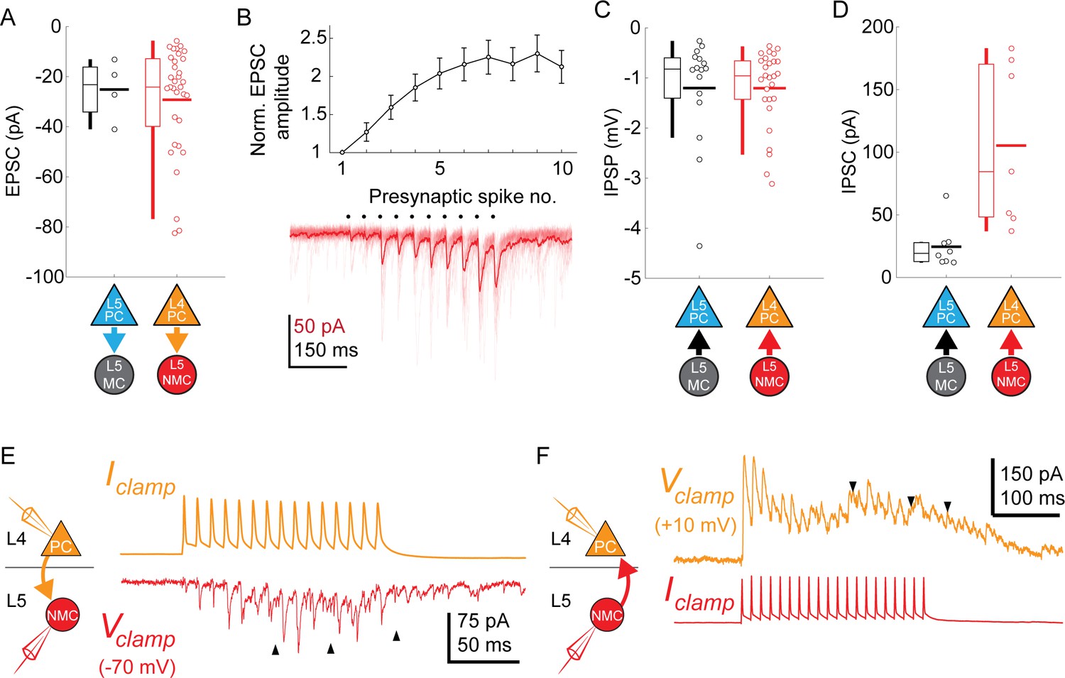
Synaptic properties of L5 SST connections .
(A) Swarm plots and Tukey box plots of evoked EPSC amplitude in connections onto L5 MCs (black) and L5 NMCs (red), measured as the largest EPSC evoked during a train of presynaptic firing at 70 Hz. (B) Facilitation dynamics of EPSCs onto L5 NMCs. Bottom: example of facilitating EPSCs in response to a train of 10 spikes at 70 Hz in an L4 PC. Top: Mean EPSC amplitude evoked in L5 NMCs while stimulating L4 PCs at 70 Hz, normalized to EPSC amplitude after the initial spike. Errorbars represent mean ±S.E.M. (C) Swarm plots and Tukey box plots of evoked IPSP amplitude in connections from L5 MCs (black) and L5 NMCs (red) onto L4/L5 PCs. (D) As in D, but for IPSCs recorded in L4/L5 PCs (holding potential +10 mV) using a Cs-based internal. Unlike IPSPs, IPSCs evoked by L5 NMCs onto L4PCs are stronger than those evoked by L5 MCs onto L5 PCs; this may reflect differences in space clamp error when recording from L4 PCs vs L5 PCs. (E) Sustained high frequency spiking in L4 PCs appeared to evoke asynchronous EPSCs in L5 NMCs (indicated by black arrows) which continued even after the cessation of spiking. (F) As in C, but for L5 NMC -to-L4PC connections. Sustained high frequency spiking in L5 NMCs appeared to evoke asynchronous IPSCs in L4 PCs (indicated by black arrows) which continued even after the cessation of spiking.
Figure 5 with 1 supplement
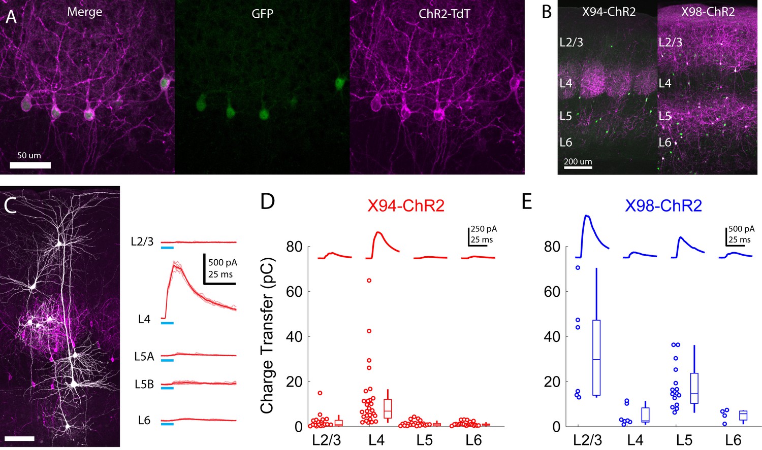
Cre-DOG enables optogenetic control of SST subtypes targeting different cortical layers.
(A) Confocal image of cortical section from an X94 mouse injected with Cre-DOG AAVs (AAV2/8.EF1a.C-CreintG WPRE.hGH and AAV2/8. EF1a. N-Cretrcintc WPRE.hGH) along with AAV9.CAGGS.Flex.ChR2-tdTomato.WPRE.SV40. Left: X94- GFP cells (green). Middle: ChR2-TdT expression (magenta). Right: Merged image (B) Side by side comparison of X94-ChR2 mice and X98-ChR2 mice showing laminar differences in localization of ChR2-TdT + axons (C) Recording light-evoked IPSCs in X94-ChR2 slices. Left: post-hoc confocal image showing recorded neurons (white) and ChR2-TdT + NMCs (magenta). Right: example traces of light-evoked IPSCs recorded in neurons in different layers (D) Median charge transfer of evoked IPSCs in each PC recorded in X94-ChR2 slices, grouped by layer and accompanied by box and whisker plots. Top inset: grand average IPSC (E) As in D, but for X98-ChR2 mice.
Figure 5—figure supplement 1
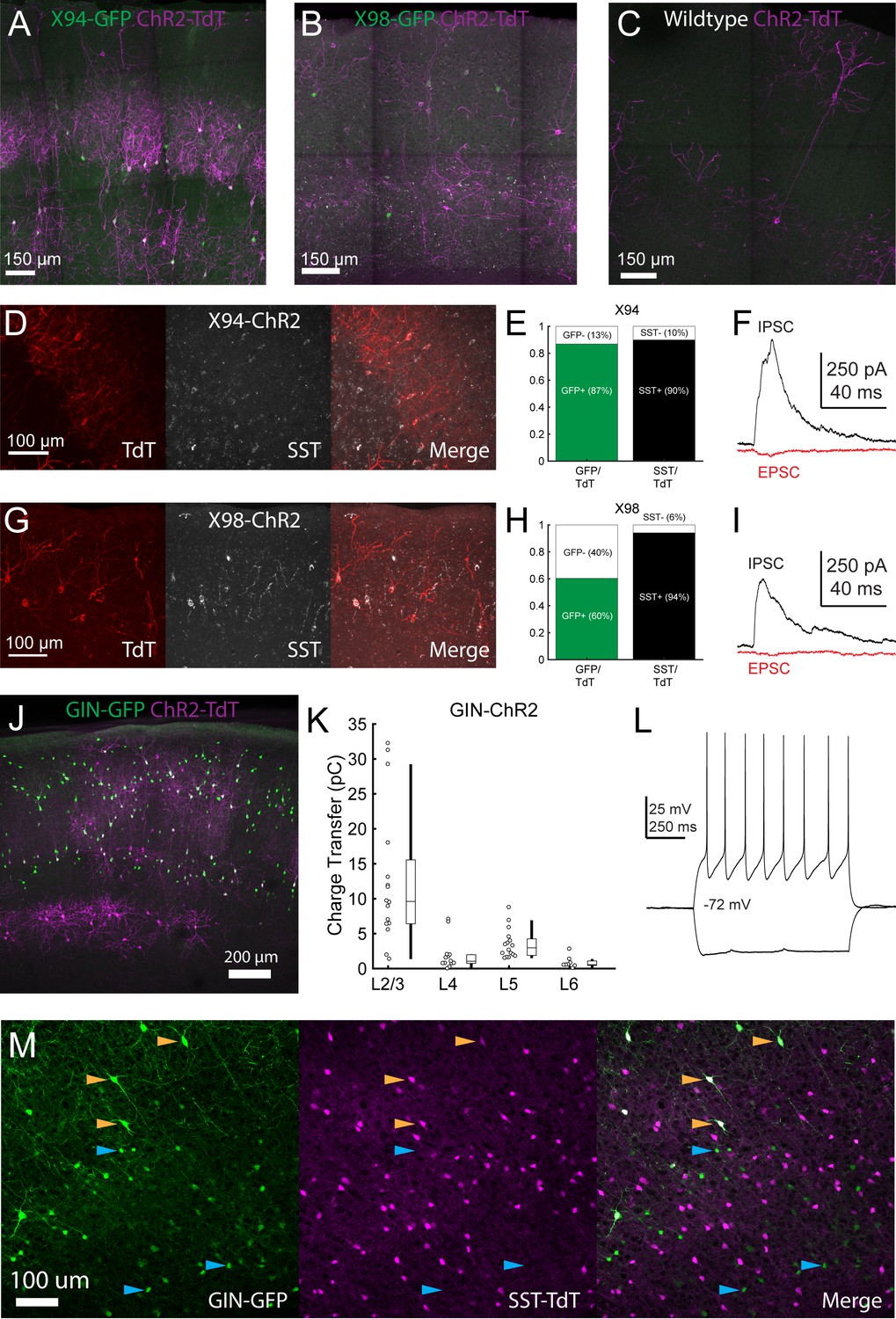
Validation of Cre-DOG for optogenetic manipulation of SST subtypes in X94, GIN, and X98 mice.
(A) Max projection of confocal images of barrel cortex of an X94 mouse injected with Cre-DOG AAVs (AAV2/8.EF1a.C-CreintG WPRE.hGH and AAV2/8. EF1a. N-Cretrcintc WPRE.hGH) along with AAV9.CAGGS.Flex.ChR2-tdTomato.WPRE.SV40 showing expression of GFP (green) and ChR2-TdT (magenta) expression. (B) As in A, but for an X98 mouse. (C) As in A, but for a wildtype mouse. (D) Immunohistochemical staining for SST in X94-ChR2 mice. Left: ChR2-TdT expression (red). Middle: SST staining (white) Right: Merge (E) Quantification of the fraction of TdT +cells in which GFP (left, green bar) and SST (right, black bar) was observed. (F) Example EPSC and IPSC traces recorded in an L4 neuron during photostimulation in a slice from an X94-ChR2 mouse. (G - I) As in D - F, but for X98-ChR2 mice. (J) Max projection of a confocal image from a GIN mouse injected with Cre-DOG AAVs (AAV2/8. EF1a.C-CreintG WPRE.hGH and AAV2/8. EF1a. N-Cretrcintc WPRE.hGH) along with AAV9.CAGGS.Flex.ChR2-tdTomato.WPRE.SV40 showing expression of GFP (green) and ChR2-TdT (magenta) expression. (K) Median charge transfer of evoked IPSCs in each PC recorded in GIN-ChR2 slices, grouped by layer and accompanied by box and whisker plots. (L) Example current injection traces from an L6, TdT +non Martinotti neuron recorded in a GIN-ChR2 slice. (M) Confocal images from a triple transgenic GIN; SST-TdT animal. Left: GFP (green). Middle: TdT (magenta). Right: merge. Yellow arrows indicate TdT +cells with bright GFP expression, which are likely MCs. Blue arrows indicate TdT- cells with dimmer GFP expression, which are preferentially located in L6.
Figure 6 with 2 supplements

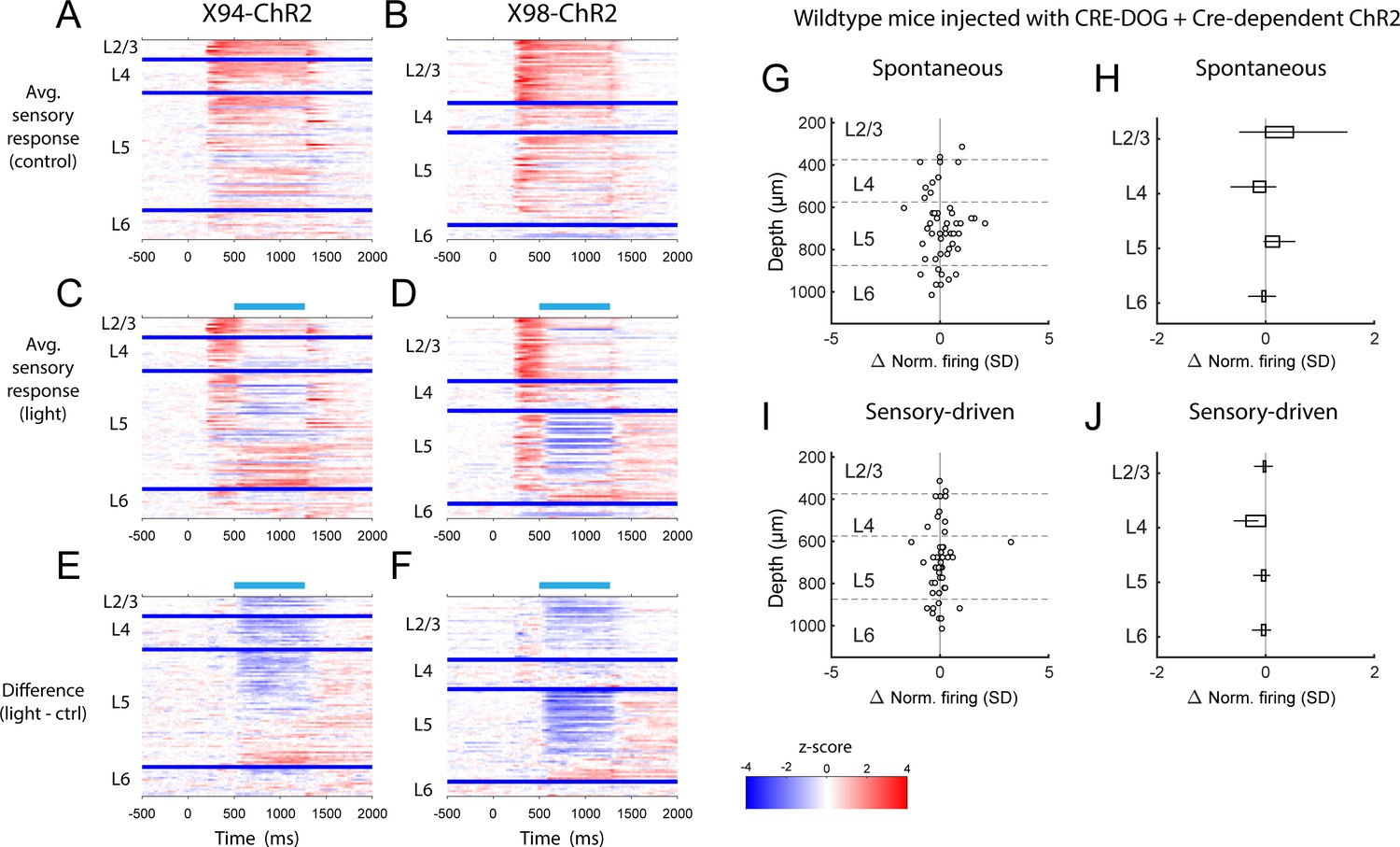
Differential layer-specific modulation of cortical activity by optogenetic activation of NMCs and MCs in vivo.
(A) Raster plots showing activity in example RS units recorded from different layers in X94-ChR2 and X98-ChR2 mice. Black rasters show trials with no stimulus that is spontaneous activity. Colored rasters show trials with photostimulation of X94-ChR2 (red) or X98-ChR2 (blue). Light blue region indicates photostimulation period. (B) Grand averages of z-scored RS unit activity in L2/3, L4, L5, and L6 showing spontaneous activity (gray) and activity on photostimulation trials (red, X94-ChR2; blue, X98-ChR2). Responses have been smoothed with a 100 ms alpha kernel and downsampled to 50 Hz. Shaded regions indicate 95% confidence interval. (C) As in A, but for sensory-driven activity from trials in which a vertical pole is presented to the whiskers as a tactile stimulus (D) As in B, but for sensory-driven activity (E) Change in normalized spontaneous firing of RS units versus depth below pia for X94-ChR2 (left, red) and X98-ChR2 (right, blue) mice. Large circles and small dots indicate units that were respectively significantly or not significantly modulated by optogenetic stimulation. (F) Mean change in normalized firing rate by layer for X94-ChR2 (red bars) and X98-ChR2 (blue bars). Errorbars indicate 95% confidence interval. (G) As in E, but for change in sensory-driven activity (H) As in F, but for change in sensory-driven activity.
Figure 6—figure supplement 1
PSTHs of RS unit sensory responses during in vivo optogenetic manipulation of MCs and NMCs.
(A) Heatmaps showing the mean normalized firing rate of all RS units recorded in X94-ChR2 mice during sensory stimulation, in the absence of optogenetic stimulation. Each row represents a single unit, and units are grouped according to the layer in which they were recorded. Within each layer group, units are sorted based on the degree to which they are modulated by optogenetic stimulation. Thick blue bars indicate divisions between layers. (B) As in A, but for RS units recorded in X98-ChR2 mice. (C) Heatmaps showing the mean normalized firing rate of all RS units recorded in X94-ChR2 mice during sensory stimulation along with optogenetic stimulation. Units are arranged as in A. Light blue bar indicates the period when optogenetic stimulation occurred. (D) As in C, but for RS units recorded in X98-ChR2 mice. (E) Heatmaps showing the difference in the mean normalized firing rate of all RS units recorded in X94-ChR2 mice between sensory stimulation with and without optogenetic stimulation, for example panel C subtracted from panel A. (F) As in E, but for RS units recorded in X98-ChR2 mice. (G) Change in normalized spontaneous firing of RS units versus depth below pia for wildtype mice injected with the same viral cocktail as X94/X98-ChR2 mice (H) Mean change in normalized spontaneous firing rate by layer for wildtype mice. Errorbars indicate 95% confidence interval. No significant effects were observed in any layer. (I) As in G, but during sensory-driven activity. (J) As in H, but during sensory-driven activity. No significant effects were observed in any layer.
Figure 6—figure supplement 2

PSTHs of FS unit sensory responses during in vivo optogenetic manipulation of MCs and NMCs.
(A) Heatmaps showing the mean normalized firing rate of all FS units recorded in X94-ChR2 mice during sensory stimulation, in the absence of optogenetic stimulation. Each row represents a single unit, and units are grouped according to the layer in which they were recorded. Within each layer group, units are sorted based on the degree to which they are modulated by optogenetic stimulation. Thick blue bars indicate divisions between layers. (B) As in A, but for FS units recorded in X98-ChR2 mice. (C) Heatmaps showing the mean normalized firing rate of all FS units recorded in X94-ChR2 mice during sensory stimulation along with optogenetic stimulation. Units are arranged as in A. Light blue bar indicates the period when optogenetic stimulation occurred. (D) As in C, but for FS units recorded in X98-ChR2 mice. (E) Heatmaps showing the difference in the mean normalized firing rate of all FS units recorded in X94-ChR2 mice between sensory stimulation with and without optogenetic stimulation, for example panel C subtracted from panel A. (F) As in E, but for FS units recorded in X98-ChR2 mice. (G) Change in normalized spontaneous firing of FS units versus depth below pia for X94-ChR2 (left, red) and X98-ChR2 (right, blue) mice. (H) Mean change in normalized firing rate by layer for X94-ChR2 (red bars) and X98-ChR2 (blue bars). Errorbars indicate 95% confidence interval. (I) As in G, but during sensory stimulation. (J) As in H, but during sensory stimulation. (K) Examples of L4 (purple) and L5 (black) FS cells recorded in X94-ChR2 slices under pharmacological blockade of glutamate. Traces show the average response to X94-ChR2 stimulation, which occurs during the light blue bar. Cells were recorded using a high chloride internal solution and voltage clamped at −70 mV; inward synaptic currents presumably reflect monosynaptic GABAergic conductances. (L) Under the conditions described in K, X94-ChR2 stimulation evoked a significantly larger amount of charge transfer in L4 FS cells (n = 7) than in L5 FS cells (n = 16; p=0.0021, student’s T-test).
Figure 7 with 1 supplement

Single cell RNA sequencing of X94 and SST cells.
(A) Single-cell RNA-seq was performed on SST-TdTomato+ and GFP+/tdTomato+ cells FACS-purified from primary somatosensory cortex of X94-eGFP;Sst-cre;LSLtdTomato mice. Cells were clustered using the Louvain algorithm and organized into vertical columns based on their cluster identity (top bar), with distribution of GFP+/tdTomato +cells indicated below. Horizontal rows correspond to mRNA expression for highly differentially expressed genes that were selected as cluster classifiers. (B) Triple-label RNA in situ hybridizations were performed on X94-eGFP;Sst-cre;LSLtdTomato mice to validate the predictions made by single-cell RNA-seq. The table shows quantitation of cells co-labeled with probes for selected marker genes, GFP and tdTomato (a proxy for Sst expression). Representative image shows overlapping signals from cluster classifier Hpse, GFP and tdTomato. Insets show examples of triple-positive cells at higher magnification. (C) Summary of laminar distribution of X94 cells cluster classifier/tdTomato double-positive cells based on tracing and scoring positions of labeled cells across three animals for each condition. Horizontal lines represent estimated positions of laminar boundaries. Left-hand panel shows localization of X94 NMCs using anti-GFP for X94 cells and anti-dsRed for Sst-tdTomato cells. Histograms give normalized frequency values for cluster classifier+/tdT +cells for each indicated cortical layer.
Figure 7—figure supplement 1
Comparison of cortical SST neuron clusters predicted by two independent analyses.
Clusters predicted from the single-cell RNA-sequencing experiments described here (left) were compared to the clusters identified in an analysis of SST neurons by Tasic et al. (2017) (right) using the method described in Kiselev et al. (2018). The differences in outputs can mostly be accounted for by the splitting of the clusters identified in the present analysis, which could be due to the different sequencing platforms used (droplet-based 3’ end sequencing vs. full coverage Smart-seq), sequencing depth (low vs. high), and/or cortical area (primary somatosensory cortex vs. primary visual cortex +anterior lateral motor cortex).
Author response image 1
Author response image 2
Author response image 3
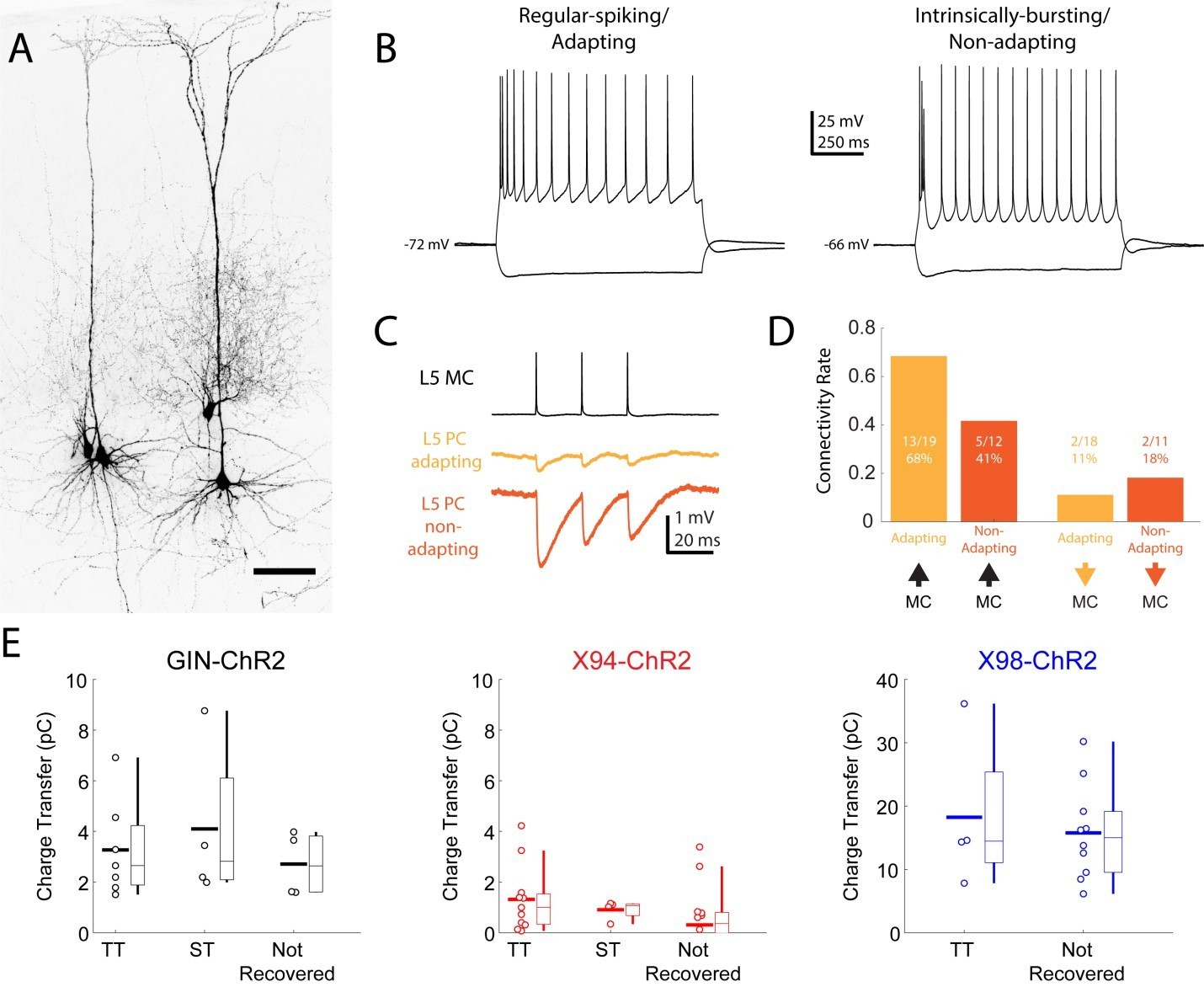
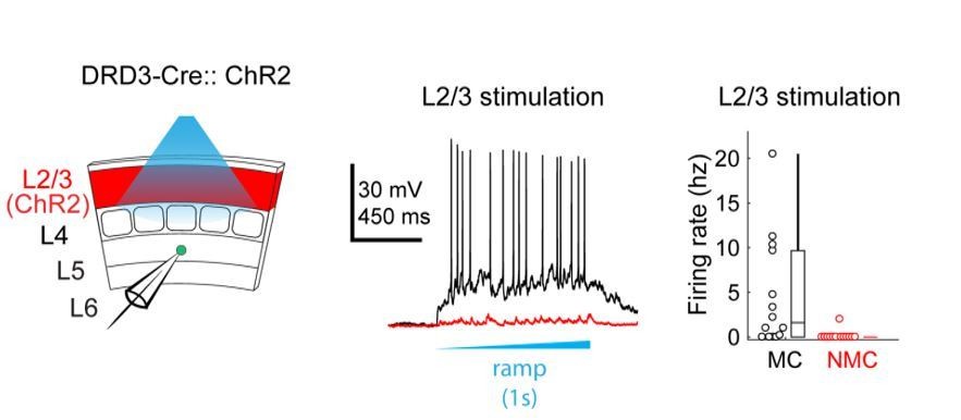
Connectivity of MCs and NMCs with L5 PC subtypes.
(A) Post-hoc confocal image showing biocytin fills from two paired recording experiments in connections were tested between an NMC and an ST L5 PC (left) and between an NMC and a TT L5 PC (right). (B) Example traces showing different spiking phenotypes in response to current injection. (C) Example IPSP traces from an adapting L5 PC (putatively ST) and a non-adapting L5 PC (putatively TT) showing diverging connectivity from the same MC onto both L5 PC subtypes. (D) Connectivity rates for MC to L5 PC inhibitory connections (left) and L5 PC to MC excitatory connections (right). (E) Inhibitory charge transfer observed in L5 PC subtypes in response to CRE-DOG based optogenetic stimulation of GIN, X94, and X98 cells. Each point in the swarm plots indicates the median charge transfer observed in a single L5 neuron; bold horizontal line indicates mean value for each distribution.
Author response image 4
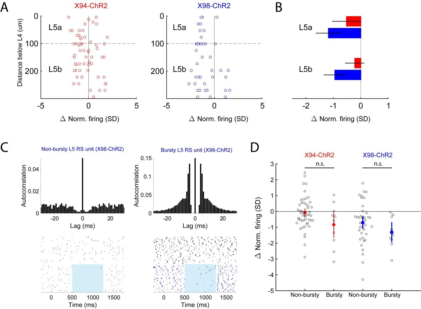
Analysis of optogenetic effects on L5 PCs in vivo.
(A) Plot of normalized change in firing during optogenetic stimulation versus electrode depth for regular spiking single units recorded in X94-ChR2 and X98-ChR2 mice. (B) Bar plots showing population effect size of optogenetic stimulation (mean ± 95% confidence interval) on regular spiking single units in L5a and L5b for X94-ChR2 (red) and X98-ChR2 (blue) experiments. (C) Example raster plots and autocorrelograms of a non-bursty L5 unit and a bursty L5 unit. (D) Swarm plot showing the normalized change in firing during optogenetic stimulation for bursty and non-bursty units in X94-ChR2 and X98-ChR2 mice. Colored points/errorbars show effect size (mean ± 95% confidence interval) in each population.
Tables
Table 1
Connection rates for MCs and NMCs recorded in different transgenic lines; related to Figure 4.
Left columns show paired recording data collected using the GIN and X94 lines to respectively target MCs and NMCs in L5. Right columns show the same data and additionally include data collected using the SST-TdT line, with L5 SST cells classified as putative MCs or NMCs based on their intrinsic properties. Columns not displaying p values show the number and fraction of SST-PC pairs in which a monosynaptic connection was detected for a given condition.
| GIN + X94 | GIN + X94+classified SST-TdT | All SST-TdT | |||||
|---|---|---|---|---|---|---|---|
| MCs | NMCs | P | MCs | NMCs | P | ||
| L5SST→L4PC | 4/47 9% | 21/34 62% | 1.6 · 10−4 | 4/68 6% | 36/67 54% | 2.0 · 10−5 | 15/55 27% |
| L4PC→L5SST | 0/50 0% | 13/27 48% | 5.8 · 10−4 | 1/95 1% | 39/72 54% | <10−5 | 27/91 30% |
| L5SST→L5PC | 19/38 50% | 1/38 3% | 2.8 · 10−4 | 24/46 52% | 2/65 3% | <10−5 | 19/67 28% |
| L5PC→L5SST | 2/22 9% | 0/33 0% | 0.1431 | 4/29 14% | 1/60 2% | 0.02 | 5/55 9% |
Table 2
Summary of expression in SST reporter lines.
Four mouse reporter lines were used in this study to target SST neurons and subtypes. Each row provides a description of the expression observed in the barrel cortex in a particular layer for each reported line.
| SST-TdT | GIN | X94 | X98 | |
|---|---|---|---|---|
| L2/3 | All SST cells | Dense, MCs | Very sparse | Sparse, MCs |
| L4 | All SST cells | Sparse, NMCs | Dense, NMCs | Very sparse |
| L5 | All SST cells | Moderate, preferentially in 5A, MCs | Moderate, preferentially in 5B, NMCs | Dense, preferentially in 5B, MCs |
| L6 | All SST cells | Sparse, Dim labeling of (non-SST?) cells | Sparse, preferentially in upper 6A, NMCs | Moderate |
Key resources table
| Reagent type (species) or resource | Designation | Source or reference | Identifiers | Additional information |
|---|---|---|---|---|
| Genetic reagent (Mus musculus) | Scnn1-tg3-Cre line | Jackson Labs | #009613 | |
| Genetic reagent (Mus musculus) | Emx1-IRES-Cre line | Jackson Labs | #005628 | |
| Genetic reagent (Mus musculus) | PV-IRES-cre line | Jackson Labs | #008069 | |
| Genetic reagent (Mus musculus) | SST-IRES-cre line | Jackson Labs | #013044 | |
| Genetic reagent (Mus musculus) | GIN line | Jackson Labs | #003718 | |
| Genetic reagent (Mus musculus) | X94-GFP line | Jackson Labs | #006334 | |
| Genetic reagent (Mus musculus) | X98-GFP | Jackson Labs | #006340 | |
| Genetic reagent (Mus musculus) | Ai9 Rosa-LSL-tdTomato line | Jackson Labs | #007909 | |
| Recombinant DNA reagent | AAV9.CAGGS.Flex. ChR2-tdTomato.WPRE.SV40 | University of Pennsylvania Vector Core | ||
| Recombinant DNA reagent | AAV9-2YF-hSyn-DIO-ChrimsonR-mRuby2-Kv2.1 | This lab | Available at Addgene(Plasmid #105448);Described in Pégard et al. (2017) | |
| Recombinant DNA reagent | AAV2/8.EF1a.C-CreintG.WPRE.hGH | Massachusetts Ear and Eye Infirmary Vector Core | ||
| Recombinant DNA reagent | AAV2/8.EF1a.N-Cretrcintc.WPRE.hGH | Massachusetts Ear and Eye Infirmary Vector Core | ||
| Antibody | Rat monoclonal anti-somatostatin primary | Millipore | MAB354 | 1:1000 dilution |
| Antibody | Goat polyclonal anti-rat Alexa 647 secondary | Life Technologies Corporation | A21247 | 1:200 dilution |
| Sequence-based reagent | tdTomato ISH probe | ACDBiotechne | 317041-C1 and C2 | |
| Sequence-based reagent | Calb2 ISH probe | ACDBiotechne | 313641 C1 | |
| Sequence- based reagent | Hpse ISH probe | ACDBiotechne | 412251-C1 | |
| Sequence- based reagent | Tacr1 ISH probe | ACDBiotechne | 428781 C2 | |
| Sequence-based reagent | Timp3 ISH probe | ACDBiotechne | 471311-C2 | |
| Sequence- based reagent | Pld5 ISH probe | ACDBiotechne | custom C2 | |
| Sequence-based reagent | Crh ISH probe | ACDBiotechne | 316091 C1 | |
| Sequence-based reagent | Calb1 ISH probe | ACDBiotechne | 428431 C2 | |
| Sequence- based reagent | eGFP-o4 ISH probe | ACDBiotechne | 538851-C3 |
Additional files
-
Supplementary file 1
Table of differentially expressed genes showing one-vs-all contrasts for each transcriptomic cluster, with log fold change, p-value, and multiple comparisons adjusted p-value for each gene in each contrast.
- https://doi.org/10.7554/eLife.43696.025
-
Transparent reporting form
- https://doi.org/10.7554/eLife.43696.026
Download links
A two-part list of links to download the article, or parts of the article, in various formats.
Downloads (link to download the article as PDF)
Open citations (links to open the citations from this article in various online reference manager services)
Cite this article (links to download the citations from this article in formats compatible with various reference manager tools)
Complementary networks of cortical somatostatin interneurons enforce layer specific control
eLife 8:e43696.
https://doi.org/10.7554/eLife.43696


