Slow presynaptic mechanisms that mediate adaptation in the olfactory pathway of Drosophila
- University of Goettingen, Germany
- University of Konstanz, Germany
Figures
Figure 1 with 2 supplements

Cell-specific calcium dynamics in neurons of the antennal lobe.
(A) Schematics of the olfactory pathway in Drosophila. ORNs expressing the same receptor project their axons from the antenna into the same glomerulus in the antennal lobe. ORNs synapse onto uniglomerular PNs that send their axons into the calix of the mushroom body (MB) and the lateral horn (LH). (B) From top to bottom: open-closed state of the odor delivery valve. The stimulus consisted of a sequence of odor pulses and gaps with random durations between 300 ms and 2.7 s. Calcium responses to a 2 min long random stimulus (methyl acetate 10−6) measured within the same glomerulus DM1 in ORNs (orco-GAL4), PNs (GH146-GAL4) and LNs (NP2426) (shaded area indicates SEM, n = 6–7). (C) Same as in the rectangle in B. (D) Top: Calcium response from the axon terminals of PNs expressing the cytosolic calcium reporter GCaMP3 (methyl acetate at concentration 10-4.3). Several bouton-like regions of interest (ROIs) were selected in each animal (three animals, 35 ROIs), the relative change in fluorescence was calculated for each ROI and then normalized by the maximum value. Response was then averaged across all ROIs. Shaded area (barely visible) represents SEM. Bottom: response of glomerulus DM1 reported by a synaptically tagged calcium reporter Syp-GCaMP expressed in ORNs. (E) Same as in the rectangles in (D).
Figure 1—figure supplement 1
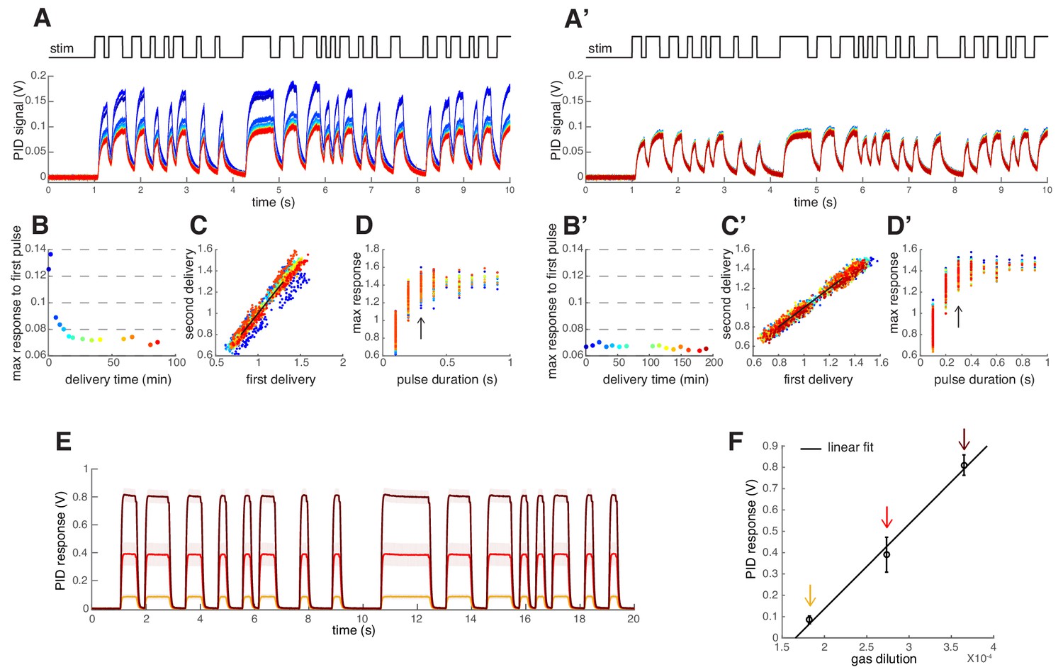
Odor Stimulus.
(A–D) Testing the reproducibility of the odor stimulus. This initial test was performed with 2 ml undiluted 2-heptanone placed in a 10 ml glass bottle. Air dilutions of the odor vapor were performed and delivered as described in Materials and methods. (A) A Photo Ionization Detector (PID, Aurora) was used to measure the odor stimulus produced by the random switching of the valve. The random sequence was applied for 1 min every 10 min 14 times (color coded). In between recordings the odor stream was directed to waste. (B) Maximum PID signal reached within the duration of the first odor pulse. The odor stimulus decays during the first 20 min of stimulation. (C) Scatterplot of the maximum PID signal calculated within each odor pulse for two stimuli delivered consecutively (color indicates consecutive 1 min long stimulus sequences). Data points on the black line indicate that the consecutive odor stimuli were identical. (D) Maximum PID response reached for the corresponding pulse duration. Please note that the stimuli used for the imaging had minimum pulse duration of 300 ms (arrow). (A’–D’) Same as (A-D) for measurements conducted on a different day after waiting 20 min for odor equilibration. (E) Mean PID signal in response to methyl acetate at 3 values of the air dilutions (C5, C8, C13, tested in random order). Shaded areas indicate SEM (n=5). (F) Mean PID response (± SEM) to the first pulse in the random sequence as a function of the gas dilution. The linear fit (black line) indicates a linear relationship between the applied odor concentration (gas dilution) and the PID readout.
Figure 1—figure supplement 2
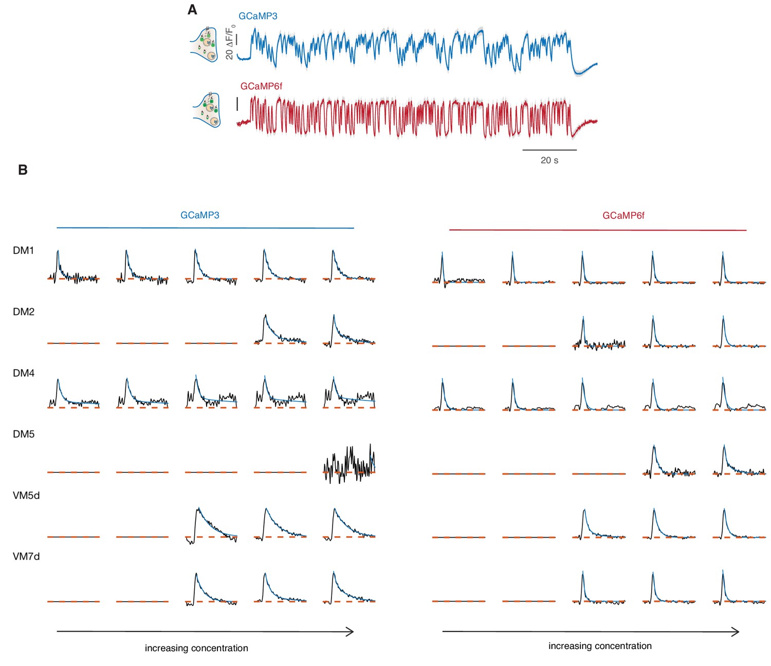
Response to sustained fluctuating stimuli reported by GCaMP6f.
(A) Calcium responses of glomerulus DM1 reported by GCaMP3 and GCaMP6f (mean and SEM, n = 6–8). These measurements were performed at the University of Konstanz where a setup very similar to the one in Göttingen was reproduced. See Materials and methods for details. (B) Linear filters (black) obtained by reverse correlation for the response of six glomeruli to increasing concentrations of methyl acetate. Either GCaMP3 or GCaMP6f are expressed in ORNs using the orco-GAL driver. An exponential function is fitted to the filter (cyan). Filters obtained with GCaMP6f are in all instances faster but differences between glomeruli are preserved. For example, VM5d shows a slower response than DM1. DM4 response is saturated at the three highest concentrations and linear filters extracted with both calcium reporters do not reach the zero indicating a slow trend in the activity. Filters are not shown for odor concentrations that elicited too weak responses in the glomerulus.
Figure 2
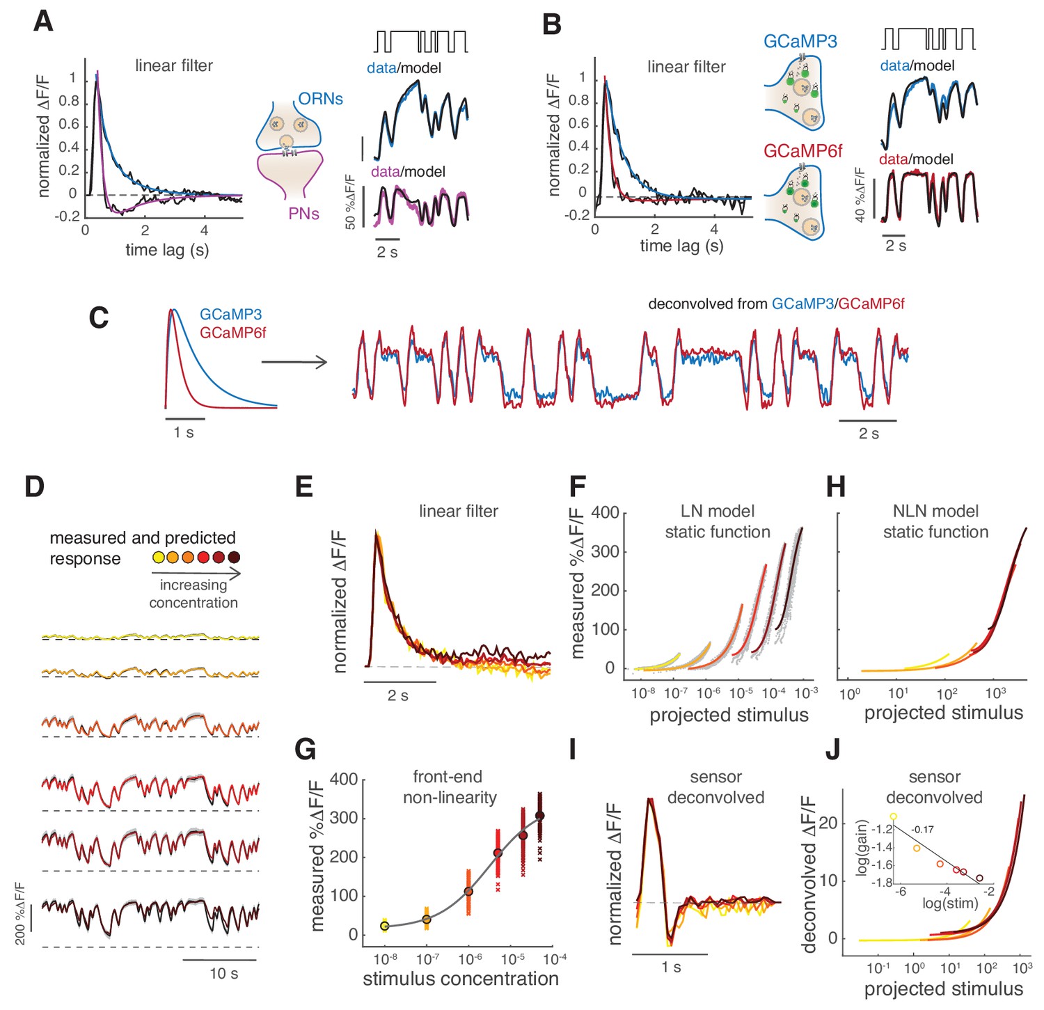
Calcium dynamics in ORNs axon terminals.
(A) Linear filter (black) of the DM1 ORNs and PNs response (methyl acetate at C04, n = 11) and fitted exponential decay (cyan ) or double exponential (purple: ). Left: measured response (black) and response predicted by a LN model (cyan/purple) for DM1 ORNs and PNs. Goodness of fit was quantified as the ratio between the mean squared residual and noise (see Materials and methods and Figure 7—figure supplement 1), here NR=0.12. (B) Linear filters (black) and fitted exponential decay (cyan/red) for the response of DM1 ORNs expressing either GCaMP3 (cyan) or GCamP6f (red). Left: mean measured response (black, n = 6-8) and response predicted by a LN model (cyan/red, NR=0.29/0.48). (C) Exponential filters used to model the dynamics of the sensor kinetics (τ = 0.7s for GCaMP6f and τ = 0.2s for GCaMP6f) and ORN calcium response deconvolved from data in (B). Results are robust to variations in the exact value of the timescale. (D) Measured (black) and predicted (colored) response for ORNs in DM1 at different concentrations of the random stimulus, increasing from yellow to dark red (n = 9–11). (E) Linear filters fitted at increasing odorant concentrations. (F) Static functions (colored) resulting from either a linear or sigmoidal fit to the instantaneous measured response as a function of the projection of the stimulus on the linear filter (gray dots, see Materials and methods). (G) Estimate of the front-end non-linearity. Crosses: peak response to each pulse in the random series for the seven stimulus concentrations. Circle: mean peak response. Gray line: Hill function fitted to the mean peak response. (H) Static functions resulting from a NLN model of the calcium response. These functions were obtained as in (F) but passing the stimulus first through the front-end non-linearity estimated in (G). (I) Linear filters calculated from the calcium signal after deconvolution of the sensor kinetics and (J) corresponding static function. Inset: logarithm of response gain quantified as the slope of the static function and plotted as a function of the logarithm of the concentration. The line indicates a linear fit and the number is the slop of the linear function.
Figure 3 with 1 supplement
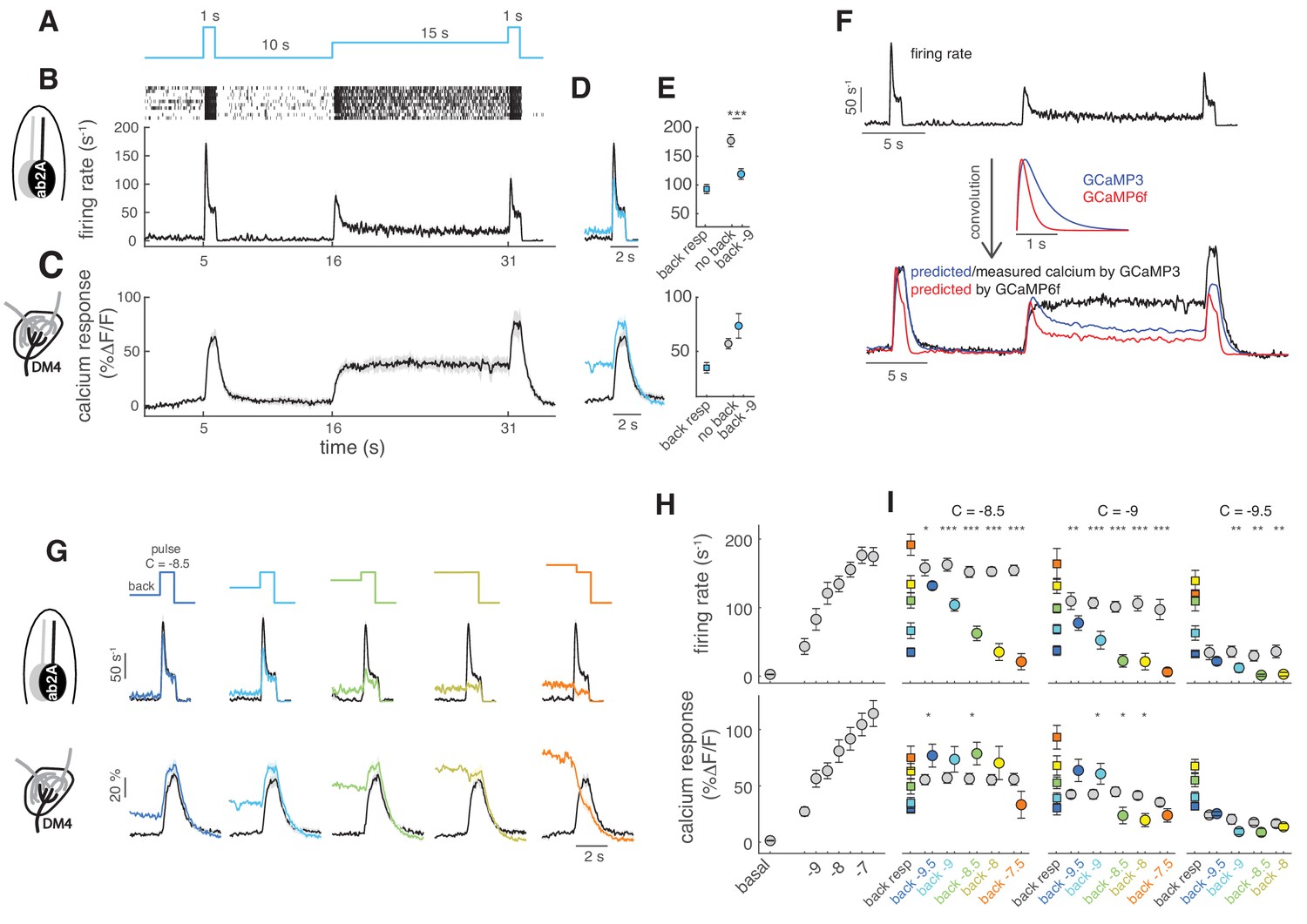
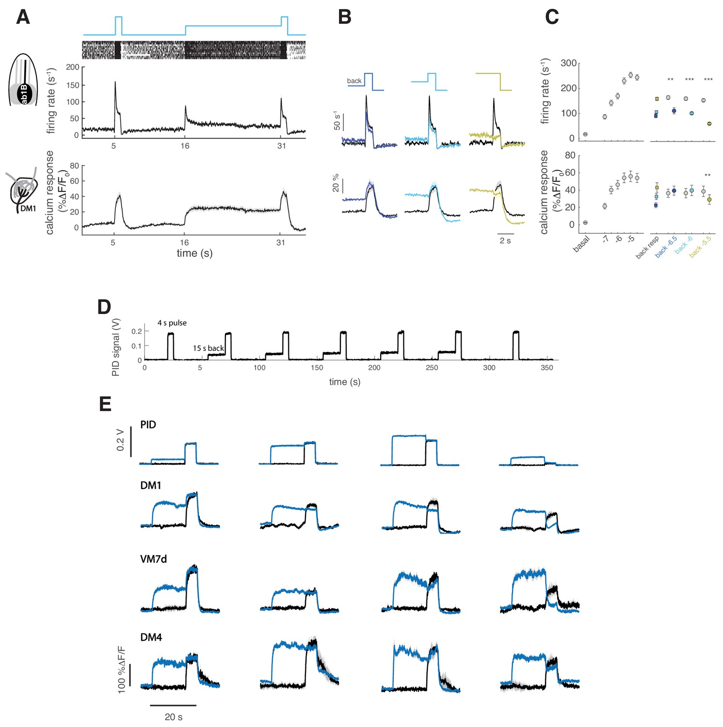
Background adaptation in ORN firing rate and calcium responses.
(A) Stimulus protocol: a pulse of methyl acetate (10-8.5 dilution) was presented first isolated and on top of a background of the same odor at lower concentration (10−9) delivered for 15 s. (B) Raster plot and mean firing rate for the spiking response of ab2A (expressing OR59b) measured in single sensillum recordings, n = 10. (C) Mean calcium response measured at the axon terminals in the corresponding glomerulus DM4, n = 8. (D) Overlay of the response to the isolated odor pulse (black) and the pulse presented on the background (cyan) for firing rate (top) and calcium (bottom). (E) Peak response to background stimulation (squares), to the isolated pulse (gray circle) and to the pulse on background (cyan circle). Paired ttest, ***p<0.001, n = 10. (F) Convolution (bottom traces) of the firing rate (top trace) with linear filters representing GCaMP3 and GCaMP6f kinetics. (G) Overlay of the response to the isolated odor pulse (black) and the pulse presented on the background (colored) for five increasing values of the background concentration, n = 8–10. (H) Dose-response curve measured as mean firing rate (n = 6–11) and mean calcium response (n = 10–11) for increasing concentrations of the isolated odor pulse. (I) Mean response to the different odor backgrounds (squares), to the isolated pulse (gray circles) and to the pulse on background (colored circles) for three pulse concentrations (reported in log scale). Paired ttest, *p<0.05, **p<0.01, ***p<0.001, n = 7–10 for firing rate and n = 6–8 for calcium responses. Shaded areas and error bars indicate SEM. Calcium responses were measured in the same flies for figure (H) and (I).
Figure 3—figure supplement 1
ORN background adaptation.
(A) Top: a pulse of methyl acetate (10−5 dilution) was presented first isolated and on top of a background of the same odor at lower concentration (10-6.5) delivered for 15 s. Middle: raster plot and mean firing rate for the spiking response of ab2A (expressing OR59b) measured in single sensillum recordings, n = 12. Bottom: mean calcium response measured at the axon terminals in the corresponding glomerulus DM1, n = 10. Shaded areas and error bars indicate SEM. (B) Overlay of the response to the isolated odor pulse (black) and the pulse presented on top of the background (colored) for three increasing values of the background concentration, (n = 10–13 for firing rate and n = 9–10 for calcium imaging). (C) Left: Dose-response curve measured as mean firing rate (n = 9–10) and mean calcium response (n = 11) for increasing concentrations of the isolated odor pulse. Right: Mean response to the different odor backgrounds (squares), to the isolated pulse (gray circles) and to the pulse on top of the background (colored circles). Paired t test, *p<0.05, **p<0.01, ***p<0.001, n = 10–13 for firing rate and n = 9–10 for calcium responses. (D) PID measurements of the stimulus sequence used for experiments with GCaMP6f. A control pulse was delivered at the beginning and at the end of the stimulus sequence. The same pulse was then presented on a background of the same odor after 15 s presentation of the odor. The test was presented five times and the stimulus was reproducible over repetitions. Odor: Methyl acetate, pulse duration is 4 s (in main Figure 3 the test pulse is 1 s). (e) Mean calcium response from single flies expressing GCaMP6f in ORNs, averaged over five repetitions in presence and absence of the background odor for different values of the background and pulse concentration, as reported by PID measurements. Results are consistent with those reported by GCaMP3 (Figure 3).
Figure 4 with 1 supplement
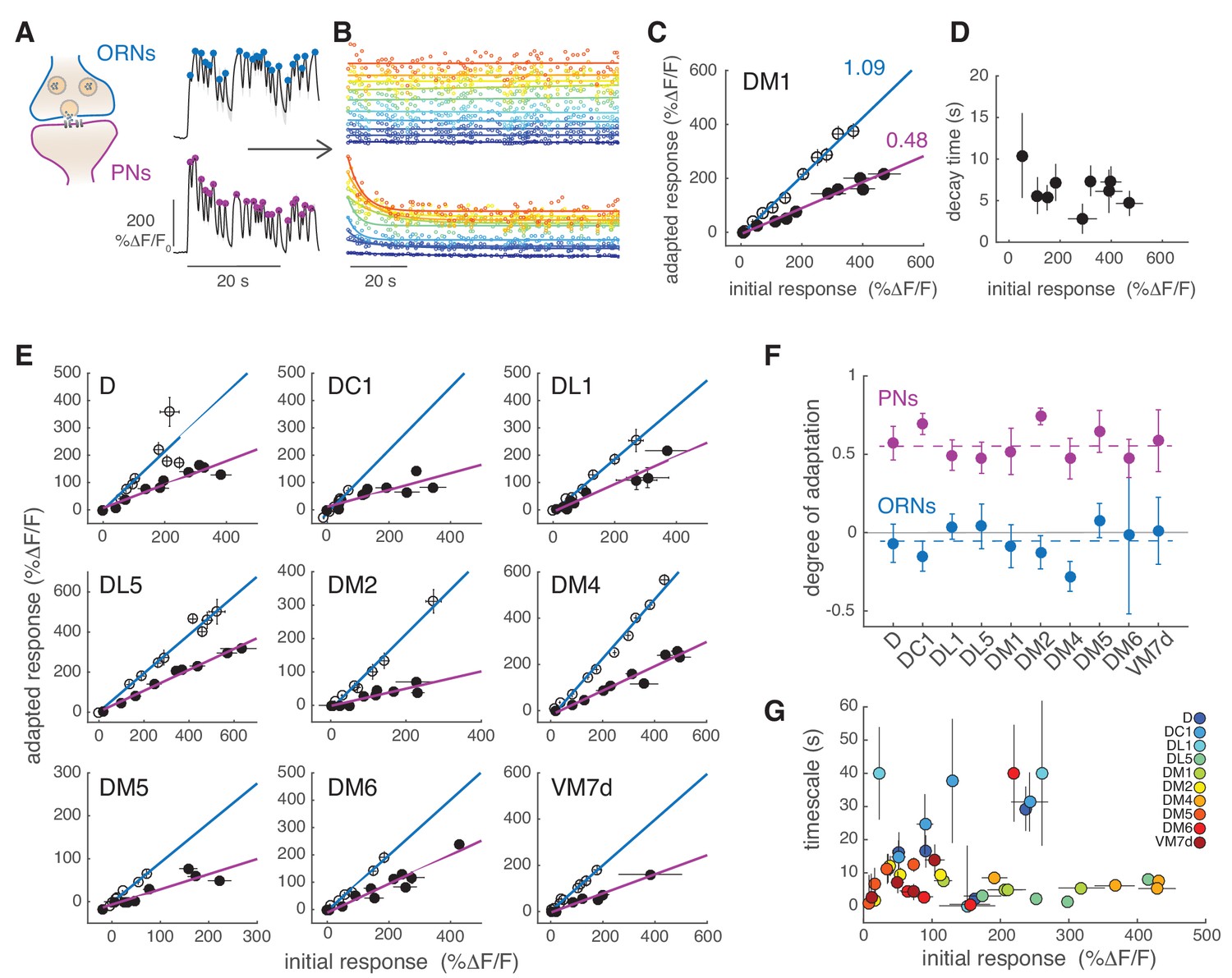
PNs adapt on slow timescales to a sustained, fluctuating odor stimulus.
(A) Initial calcium response reported by GCaMP3 to the first 30 s of random odor stimulation in ORNs and PNs within glomerulus DM1. Dots indicate the peak response to each single odor pulse in the random stimulus sequence calculated from the mean ΔF/F (n = 11, 7). (B) All trials for glomerulus DM1 were pooled, sorted by amplitude and averaged in 10 bins spanning the entire response range (see Materials and methods for detail). Peak amplitude of the mean response to each single random pulse is plotted as a function of time and color-coded by the amplitudes for ORNs (top) and PNs (bottom). Continuous lines represent linear (ORNs, ) or exponential (PNs, ) fits to the time-dependent peak responses. (C) Adapted response as a function of the initial response for ORNs (empty circles) and for PNs (filled circles). Initial and adapted responses were calculated using the fitted parameters. Error bars indicate 95% confidence intervals. Continuous lines represent a linear fit. Numbers indicate slopes of the linear relationship. (D) Adaptation time constants of PN responses for different response amplitudes estimated from the exponential fit. Error bars indicate 95% confidence intervals. (E) Adapted response as a function of the initial response for nine glomeruli and corresponding linear fit. (F) Degree of adaptation estimated as 1 minus the slope of the linear relationship between the adapted and initial response. Dashed lines indicate the mean degree of adaptation across glomeruli: -0.06 ± 0.1 for ORNs and 0.57 ± 0.1 for PNs (mean ± standard deviation). The gray continuous line indicates no adaptation. Error bars indicate 95% confidence intervals (n = 5–11). For all glomeruli, the degree of adaptation is significantly different from zero (p<0.001). (G) Adaptation timescales estimated for four odorant concentrations, color-coded by glomerulus, and plotted as a function of response amplitude. Error bars indicate 95% confidence intervals (n = 5–11). See also Figure 4—figure supplement 1. Note that a slow decay in activity that outlasted the stimulus duration was observed at the lowest and highest concentrations in DL1 and at the highest concentration in DM6. For these measurements we report confidence intervals for an exponential fit with the maximum timescale (which was set to 40 s in our analysis).
Figure 4—figure supplement 1
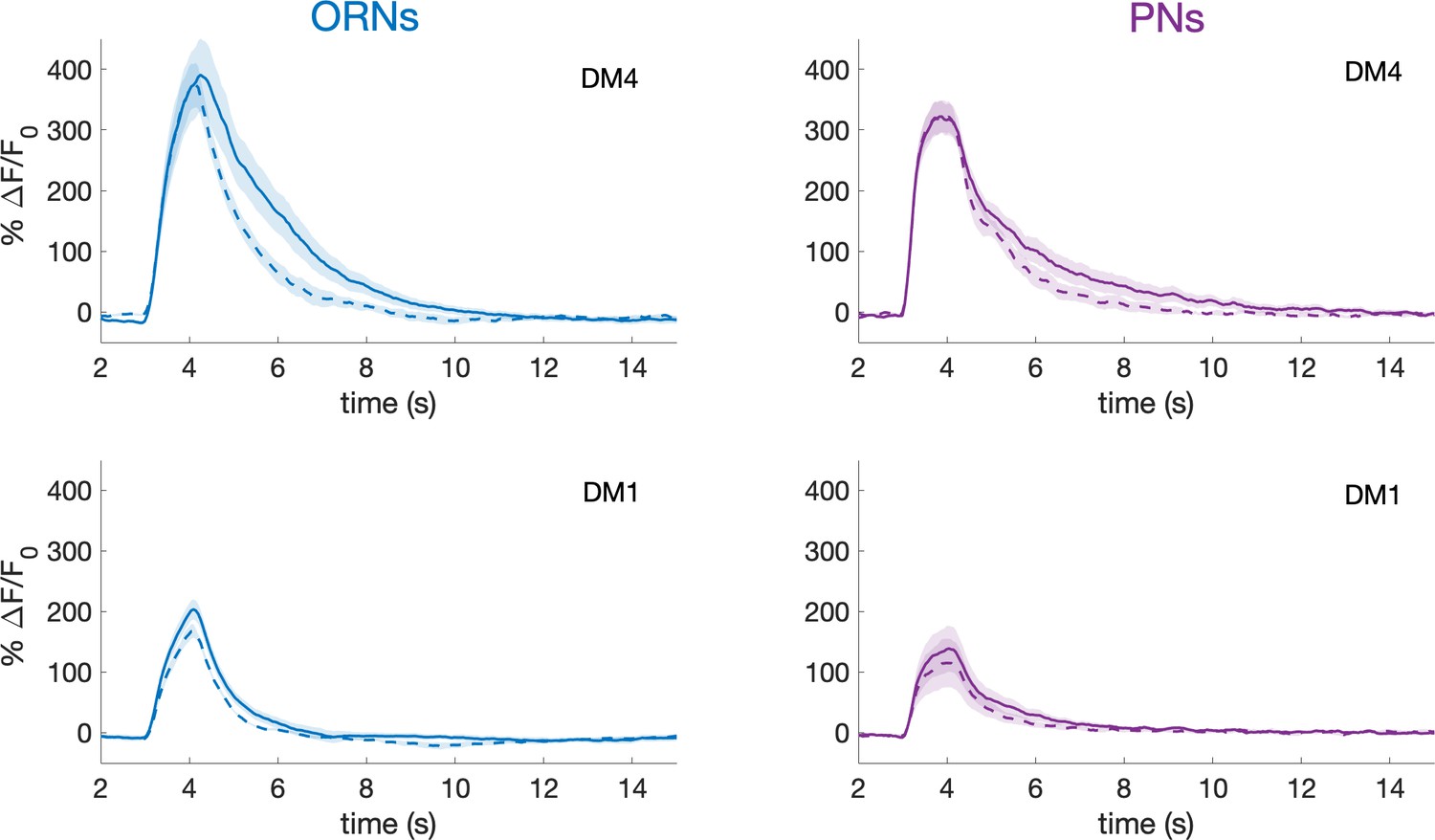
PNs activity recovers from slow adaption within a minute.
In this experiment, a single pulse of methyl acetate was delivered one minute before (continuous line) and one minute after (dotted line) the 2 min long pseudorandom stimulus. The response amplitudes in ORNs and PNs innervating glomeruli DM1 and DM4 shows no significant differences. Shaded area represents SEM, n = 6. This demonstrates that the slow adaptation observed here is a different phenomenon from the previously described habituation (Das et al., 2011).
Figure 5 with 1 supplement
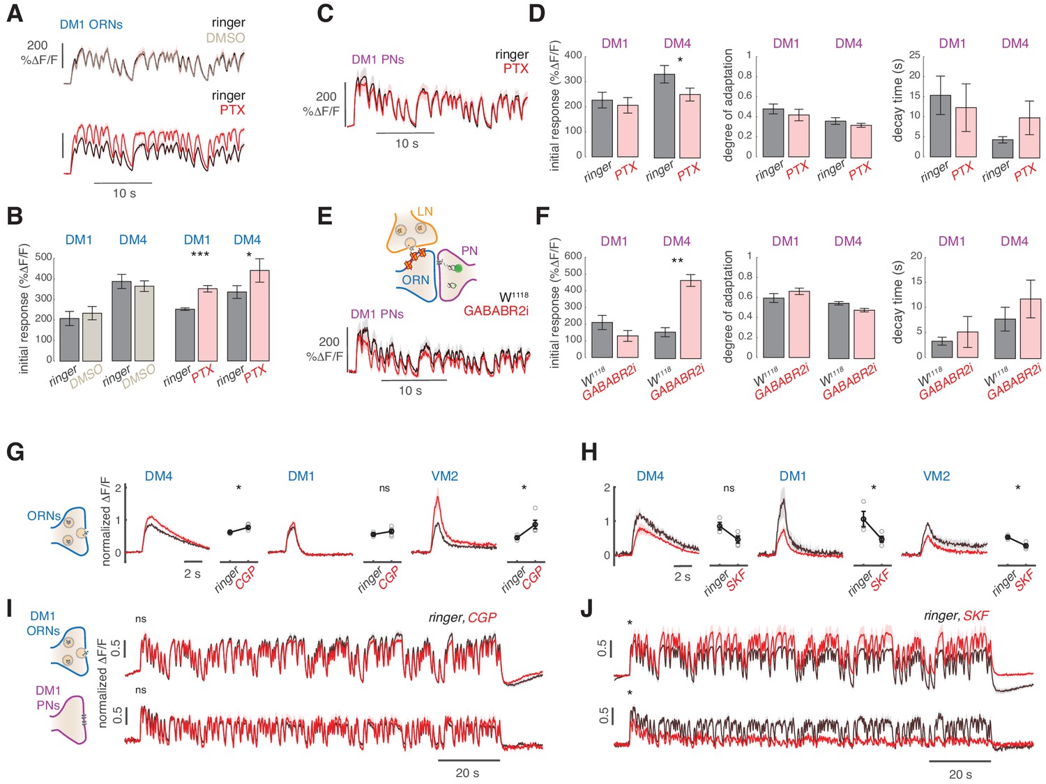
Slow adaptation in the PN calcium signal is not driven by lateral inhibition.
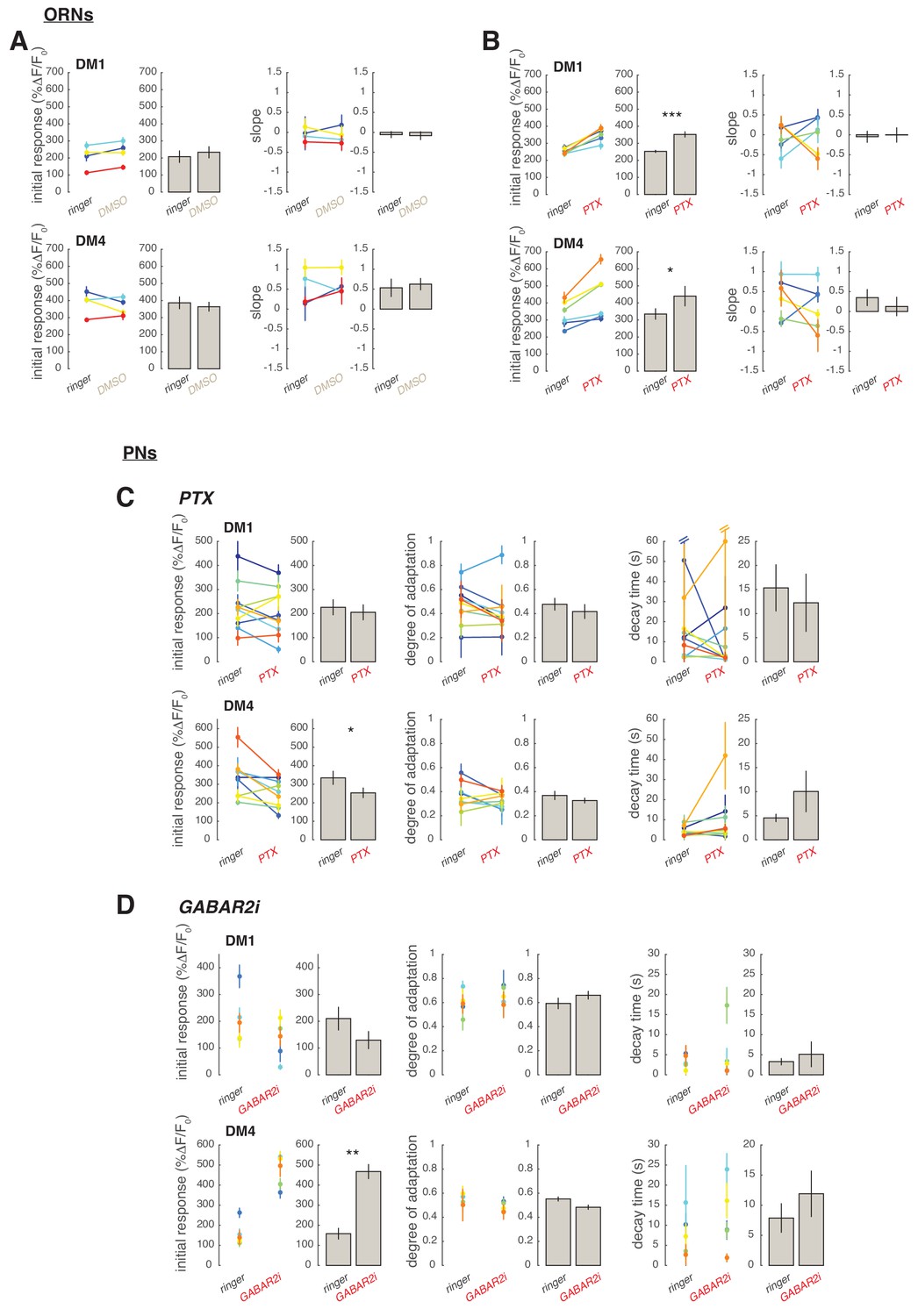
(A–D) Application of the GABA-A receptor antagonist PTX does not affect calcium adaptation in PNs. (A) Application of 5 μM PTX enhances the calcium response from ORN terminals in glomerulus DM1. Top: Calcium response to randomly fluctuating odor stimulation (methyl acetate) before and after application of an equivalent DMSO control (n = 4). Bottom: Calcium response before and after application of 5 μM PTX (n = 6). Shaded areas indicate SEM. (B) PTX enhances the response to the first odor pulse measured from ORNs in glomeruli DM1 and DM4. Paired t test, *p<0.05, ***p<0.001. Error bars indicate SEM. (C) Mean calcium signals from PNs in DM1 in response to random stimulation before (black) and after (red) PTX application. Shaded areas indicate SEM (n = 10). (D) Initial response r0, degree of adaptation , and decay timescale of PN activity under sustained random stimulation for glomeruli DM1 and DM4 before and after PTX application, calculated by fitting an exponential decay function to the peak response to each odor pulse in the random sequence (Figure 5—figure supplement 1). Error bars indicate SEM. PTX application slightly decreases DM4 response but has no effect on the other parameters (paired t test, n = 10). (E) Schematic illustration of GABA-B-R2 RNAi-mediated down-regulation and simultaneous expression of the calcium reporter GCaMP3 in PNs. Bottom: Mean calcium signal from DM1 PNs in flies expressing GABA-B-R2-RNAi and in control w1118 flies. Shaded areas indicate SEM (n = 5). (F) GABA-B-R2-RNAi expression affects the initial response r0 but not the degree of adaptation and the decay timescale of PNs activity in glomeruli DM1 and DM4 (**p<0.01, Mann-Whitney U-test, n = 5). Also see Figure 5—figure supplement 1. (G) Mean response of ORNs from DM4 and DM1 (methyl acetate 10-4.3 dilution) and VM2 (ethyl butyrate 10-7.5) to a 1 s pulse, in control flies (black) or in flies treated with 25μM CGP54626 (GABA-B antagonist). (*p<0.05, ***p<0.001, Kruskal-Wallis test, n = 3-5). In both test and control flies, the odor response was first quantified in normal ringer. The ringer was then replaced with new ringer in control flies and with ringer + CGP54626 in test flies. Odor response was tested again 8 minutes after drug application. The response in presence of the drug was then normalized to the response to the first presentation of the odor to account for fluctuation in the odor concentration. (H) Same as in (G) with 40μM SKF97541 (GABA-B agonist) (*p<0.05, **p<0.01, Kruskal-Wallis test, n = 3-4). (I) Mean response of ORNs and PNs from DM1 to a random stimulus sequence (methyl acetate 10-4.3 dilution) in ringer (black) or in CGP54626 (red). Response is normalized in each fly to the mean response to the first odor pulse obtained in ringer. No change was observed after drug application (n=6-8), similarly to control flies treated with ringer (not shown). (J) Mean response of ORNs and PNs from DM1 to a random stimulus sequence (methyl acetate 10-4.3 dilution) using ringer (black) or SKF97541 (red). Response is normalized in each fly to the mean response to the first odor pulse obtained in ringer. Response to the first odor pulse is lower in both ORNs and PNs after drug application (paired t-test, n=5-6).
Figure 5—figure supplement 1
Single trials from GABA experiments.
The calcium signal within glomerulus DM1 and DM4 in response to the 2 minutes fluctuating stimulus was quantified in individual flies. As in main Figure 4, the maximum response to each individual odor pulses within the random pulse sequence was calculated. In ORNs the maximum response as a function of time, , was then fitted by a linear function: , where indicates the initial response and the slope of a linear trend in the response amplitude. In PNs was fitted by an exponential function: , where is the degree of adaptation () and the decay timescale of the response. (A) Effect of DMSO on calcium response. Initial response and slope fitted in single trials (colored dots, error bars indicate 95% confidence intervals) and averaged across trials (gray bars ± SEM, n=4). DMSO has no significant effect on initial response and on a linear trend in the response amplitude over 2 min (paired t-test). (B) Same as (A) for PTX application. PTX significantly increases the initial response of both DM1 and DM4 (paired t-test, *p<0.05, ***p<0.001, n=6). (C) In PNs PTX application slightly decreases DM4 initial response (p<0.05) but has no effect on the degree of adaptation or on the response decay timescale (n=10). Note that in two trials confidence intervals for were extremely large suggesting that the exponential function is not a good fit for the data due to a slow superimposed linear trend. Excluding these two data points from the analysis does not affect the results. (D) In PNs expression of GABABR2-RNAi increases the initial response of DM4 (**p<0.01) but has no effect on DM1 (Mann-Whitney U-test). Degree of adaptation and timescale of the response decay are also not affected (n=5).
Figure 6 with 2 supplements
Slow adaptation in the PN calcium signal reflects slow depression in vesicle release at the ORN terminals.
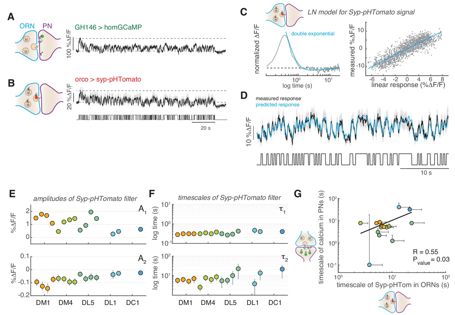
(A) Postsynaptic calcium signal in PNs measured with dHomer-GCaMP from glomerulus DM1 in response to a fluctuating odor stimulus. The gray-shaded area represents SEM. (B) Fluorescence signal of Syp-pHTomato from ORNs in DM1. (C) LN model for the Syp-pHTomato signal. Left: Normalized linear filter fitted to the data in (E) (gray) and exponential fit to the linear filter (cyan, double exponential). Right: Scatter plot of the predicted linear response and measured response (gray) and corresponding linear fit (cyan). (D) Mean Syp-pHTomato fluorescence (black, as in (C)) and response predicted by the LN model (cyan). (E) An LN model was fitted to all responses measured in five glomeruli (color coded as before) at four stimulus concentrations. The BIC was used to choose whether the linear filter shape was better captured by a simple exponential or a double exponential function. In all cases, a double exponential was selected with A1 >0 and A2 <0 (see also Figure 6—figure supplement 1). The response of DL1 to C01 and C08 and the response of DC1 to C01, C08, and C13 were too weak to fit a model. (F) The timescales of the negative exponential τ2 are always slower than that of the positive exponential τ1, indicating a slow adaptive process. (G) The slow timescale τ2 of the Syp-pHTomato signal correlates with the timescale of the slow adaptation measured in the calcium signal of postsynaptic PNs (Figure 4G). Different colors indicate different glomeruli. Error bars indicate 95% confidence intervals.
Figure 6—figure supplement 1
Linear filters for Syp-pHTomato signal from ORN terminals.
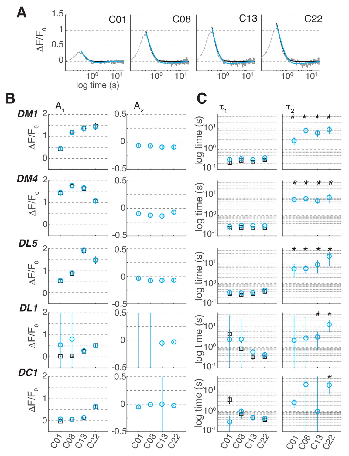
(A) Linear filter (gray) for the Syp-pHTomato signal in glomerulus DM1 at different odorant concentrations and corresponding fit with either a single (black, ) or a double (cyan,) exponential. (B) Amplitude of single (black) and double (cyan) exponential fit to the linear filter as a function of stimulus concentration in 5 glomeruli. A1 represents the amplitude of the first exponential. A2 represents the amplitude of the second exponential. Error bars indicate 95% confidence intervals. (C) Timescales of the first, τ1, and second, τ2, exponential. Error bars indicate 95% confidence intervals. Stars indicate conditions where a double exponential fits the data better than a single exponential (BIC < 0, see Materials and methods). The response of DL1 to C01 and C08 and the response of DC1 to C01, C08 and C13 are too weak to fit a model.
Figure 6—figure supplement 2
Linear correction to Syp-pHTomato fluorescence.
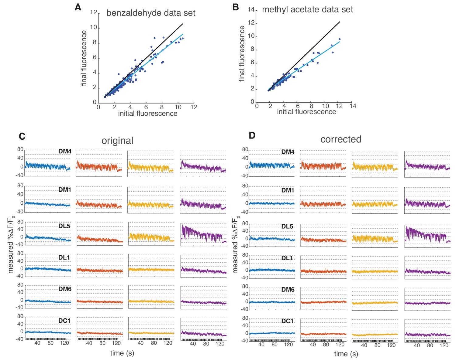
(A–B) Data for main Figure 6E and F were collected in two experimental sessions. In both cases, we noticed a drift in fluorescence probably due to bleaching of the sensor. Here, we show a scatter plot of the initial versus final baseline fluorescence (in a.u.) in the two experimental sessions for all single measurements taken (all glomeruli at all concentrations in all flies). We estimated a linear drift of 0.85 in the benzaldehyde data set and 0.7 in methyl acetate data set from the slope of the linear fit (blue line; black line indicates identity). Notice that the drift affected also non-responsive glomeruli, therefore is independent of odor response. (C) Mean change in fluorescence from 6 glomeruli at four concentrations. Shaded error bars indicate SEM. (D) Mean change in fluorescence after linear correction to the raw data.
Figure 7 with 2 supplements
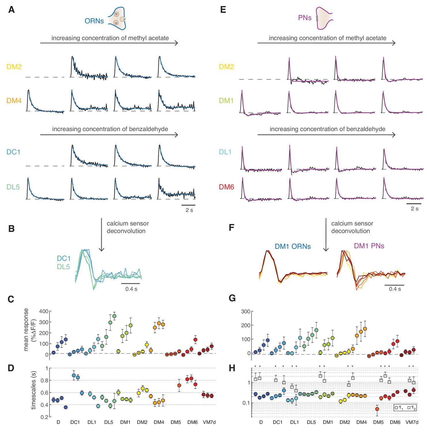
Calcium dynamics in ORNs and PNs.
(A) Linear filters (black) and corresponding exponential fit (cyan) for ORNs in four glomeruli at four concentrations of the stimulus. Two odors were used (methyl acetate and benzaldehyde) that capture the response of two non-overlapping sets of glomeruli. Responses below 10% ΔF/F were removed from further analysis because of an insufficient signal-to-noise ratio (n = 4–11). (B) Example of the linear filters obtained after deconvolution of the calcium sensor, color indicates glomerulus identity and different curves correspond to different stimulus intensities. (C) Mean responses to the fluctuating stimulus averaged over time for 10 glomeruli (color coded) at four stimulus intensities (same color). Error bars indicate standard deviations. Dashed lines indicate a threshold of 10% ΔF/F. (D) Timescale τ1 of the linear filter resulting from the exponential fit. Error bars indicate 95% confidence intervals. Timescale of the linear filters is significantly anticorrelated to mean response (R = −0.6; p<0.0004), glomerulus dependent (p<10−6) and slightly dependent on stimulus intensity (p<0.02; two-way analysis of variance). Sample size per glomerulus was: nD = 6, nDC1 = 7–8, nDL1 = 7–8, nDL5 = 7–8, nDM1 = 9–11, nDM2 = 9–11, nDM4 = 9–11, nDM5 = 7–8, nDM6 = 7–8, and nVM7d=4–6. (E) Linear filters (black) and corresponding exponential fit (purple) for PNs in four glomeruli at four concentrations of the stimulus. For each glomerulus, three models were fitted (single exponential, single exponential plus a constant, and double exponential, see Materials and methods). The model with the lowest BIC was selected. The shape of the linear filter in PNs depends on stimulus intensity. (F) Linear filter obtained from calcium responses after deconvolution of the sensor kinetics, showing that PNs filters are concentration dependent. Color indicates concentration as in Figure 2D. (G) Same as in C for PNs. (H) Timescales of the linear filter resulting from the exponential fit. Stars (*) indicate data sets that were fitted by a double exponential (model 3): in this case, a second timescales τ2 is shown, which is associated to the negative lobe pf the double exponential. τ1 is slightly correlated with the mean response (R = 0.4, p<0.02), whereas τ2 is independent from it (p>0.05). Differences between glomeruli are not significant (Kruskal-Wallis test, p>0.05). The sample size per glomerulus was as follows: nD = 7, nDC1 = 3–4, nDL1 = 6–7, nDL5 = 7–8, nDM1 = 6–7, nDM2 = 6–7, nDM4 = 6–7, nDM5 = 5–7, nDM6 = 7–8, and nVM7d = 6–7.
Figure 7—figure supplement 1

Residual-to-noise ratio in LN model cross-validation.
(A) Residual-to-noise ratio (NR) calculated as described in Materials and methods for ORN responses measured in 10 glomeruli at 4 concentrations of two odors (methyl acetate and benzaldehyde) and plotted as a function of the mean response. NR <1 indicates that the residuals of the LN model are within the variability across trials. Only in four cases NR >1. (B) Details of the model estimate for one of the recordings for which NR >1. Black: mean response of ORNs in glomerulus D to high concentration of benzaldehyde. Shaded area: SEM. Blue: prediction of the LN model showing a slight mismatch in the last 20 s of the response. (C) Measured response as a function of predicted linear response (gray dots) and fitted static function (blue line). Dots far from the curve are time points of D response that are less well fitted by the LNL model. These data show that even a poorly performing LNL model can qualitatively describe the glomerulus response. These responses were included in further analysis. (D) NR for PNs is always <1. Overall there is no obvious dependency of model prediction and response amplitude, suggesting that increased non-linearity in the response is well captured by the LN model.
Figure 7—figure supplement 2
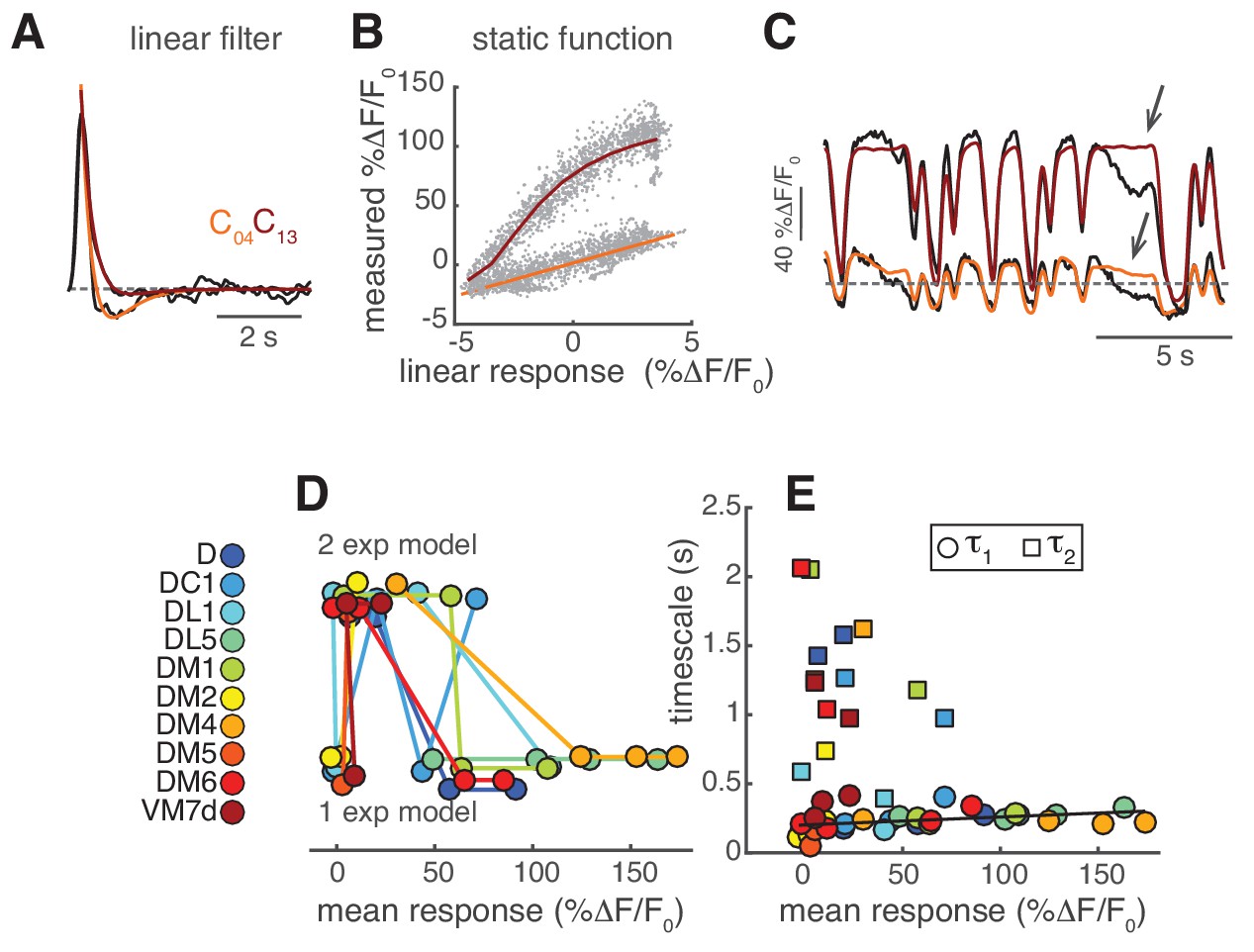
LN model for PN response.
(A) The shape of the linear filter in PNs depends on stimulus intensity. Normalized linear filters (black) for the calcium responses of PNs in DM1 to two stimulus intensities and corresponding exponential fits ( in orange for C04 and in dark red for C13). (B) Static function fitted at the two stimulus intensities: linear function in orange for C04 and Hill function in dark red for C13. (C) Measured calcium dynamics (black, n = 6–7) and calcium dynamics predicted by the corresponding LN model (orange and dark red) for the two stimulus intensities. Arrows indicate features that are not captured by the model. (D) Model selected as a function of the mean response. “1 exp” indicates a monophasic filter, “2 exp” indicates a biphasic filter. The model depends significantly on response amplitude (Kruskal-Wallis test, p<0.02). (E) Filter timescales as a function of mean response. Circles: τ1, first exponential (all models), squares: τ2 second exponential (model 3). τ1 is slightly correlated with the mean response (R = 0.4, p<0.02), whereas τ2 is independent from it (p>0.05). The black line represents a linear fit.
Figure 8 with 1 supplement
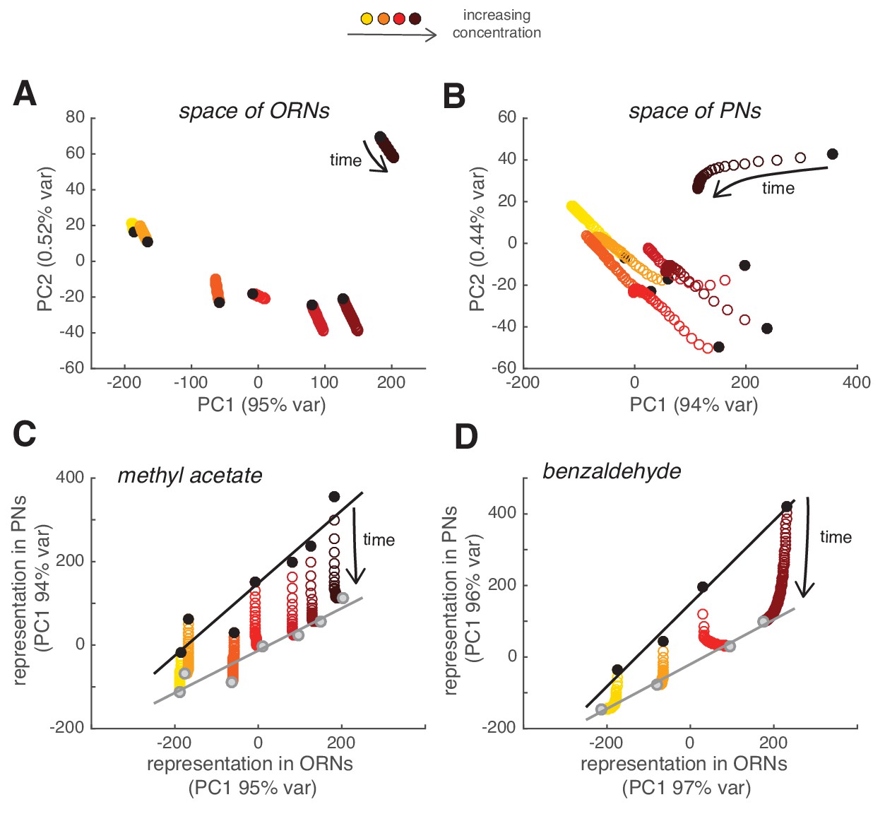
Slow depression linearly rescales odor representations in PN space.
(A) Combinatorial representation of methyl acetate represented by the first and second principal components of the ORN activity. Black circles correspond to the response to the first pulse in the random sequence; all other partially overlapping empty circles correspond to the response to subsequent odor pulses, showing how ORN odor representation is stable over 2 min. (B) Same as (A) for the response of PNs, showing how odor representations in PN space change over time. (C) Transformation of spatial representation from ORNs to PNs. Each circle represents the combinatorial response for each single odor pulse of PNs versus ORNs quantified by the first principal component. Black/gray circle: response to first/last odor pulse. Black and gray lines are linear fits to the initial and final response. (D) Same as in (C) but for benzaldehyde.
Figure 8—figure supplement 1
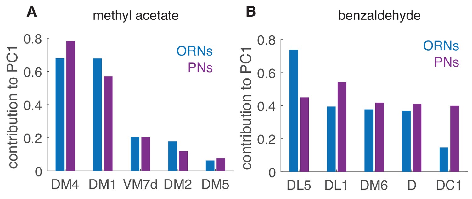
Contribution of different glomeruli to PCA Relative contributions of the different glomeruli to the PC1, here caclulated using the peak response to the single pulses as in Figure 8.
DM4 and DM1 are very sensitive to methyl acetate and they strongly contribute to the first principal component in both ORNs and PNs (A). For benzaldehyde (B), the contribution of the different glomeruli is more balanced, both in ORNs and even more in PNs.
Figure 9
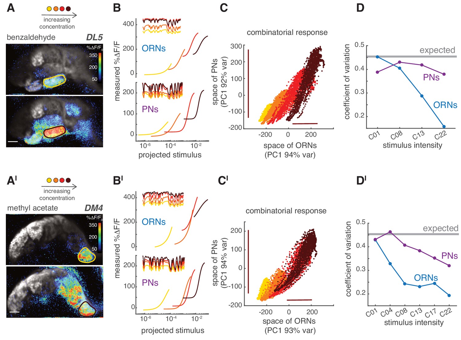
PNs accurately encode stimulus variance.
(A) Calcium increase in ORN terminals upon stimulation with benzaldehyde at two different concentrations (C01, C22). (B) Static non-linear functions fitting the relationship between measured and predicted linear calcium responses for ORNs (top) and PNs (bottom) in glomerulus DL5. As odorant concentration increases (yellow → dark red), the responses of both ORNs and PNs become more non-linear and saturates. However, PNs maintain a broader dynamic range compared to the corresponding ORNs, even when these saturate (dark red). Note that here the same binary stimulus was used for all concentrations to visualize the change in dynamic rage. (C) Scatter plot of the first principal components of the combinatorial odor representation of the odor stimuli in ORNs and PNs. Each dot represents the measured response at each time point of a 2-min-long pseudorandom stimulus. The combinatorial odor representation in the space of five responding glomeruli was almost unidimensional in both ORNs and PNs with the first principal components explaining >90% of the variance. Colors indicate odorant concentration (yellow → dark red). Bars indicate the variation in ORN and PN responses to the stronger stimulus intensity as a visual estimate of the response variance. (D) CV as a function of stimulus intensity, quantified as the standard deviation divided by the mean of the first principal component of the population response. The gray line indicates the expected CV (see Materials and methods). (A’–D’) Same as (A–D) but for methyl acetate as odorant.
Author response image 1

Author response image 2
Additional files
-
Transparent reporting form
- https://doi.org/10.7554/eLife.43735.021
Download links
A two-part list of links to download the article, or parts of the article, in various formats.
Downloads (link to download the article as PDF)
Open citations (links to open the citations from this article in various online reference manager services)
Cite this article (links to download the citations from this article in formats compatible with various reference manager tools)
Slow presynaptic mechanisms that mediate adaptation in the olfactory pathway of Drosophila
eLife 8:e43735.
https://doi.org/10.7554/eLife.43735


