Figures and data in Complementary congruent and opposite neurons achieve concurrent multisensory integration and segregation | eLife

Figures
Additional files

8 figures and 1 additional file

Figures

Figure 1 with 1 supplement

Download asset Open asset

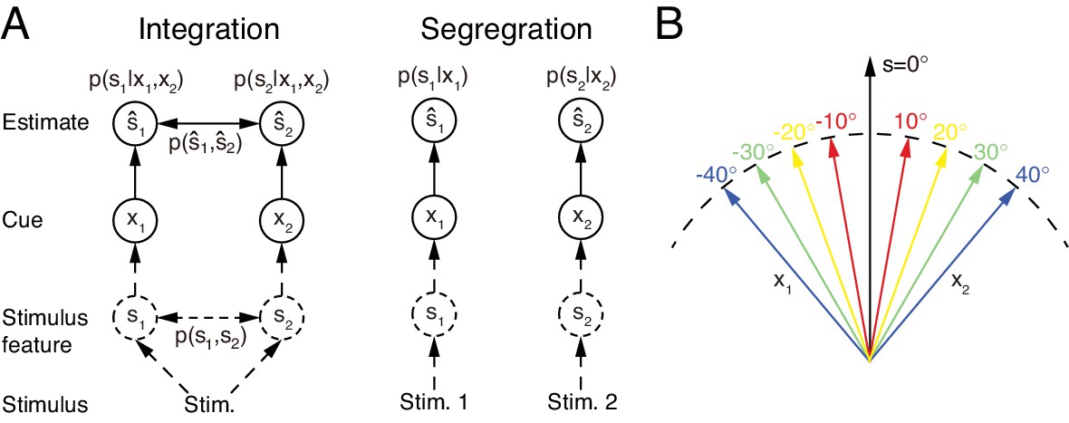
Multisensory integration and segregation.

(A) Multisensory integration versus segregation. Two underlying stimulus features $s_{1}$ and $s_{2}$ independently generate two noisy cues $x_{1}$ and $x_{2}$ , respectively. If the two cues are from the same stimulus, they should be integrated, and in the Bayesian framework, the stimulus estimation is obtained by computing the posterior $p (s_{1} | x_{1}, x_{2})$ (or $p (s_{2} | x_{1}, x_{2})$ ) utilizing the prior knowledge $p (s_{1}, s_{2})$ (left). If two cues are from different stimuli, they should be segregated, and the stimulus estimation is obtained by computing the posterior $p (s_{1} | x_{1})$ (or $p (s_{2} | x_{2})$ ) using the single cues (right). (B) Information of single cues is lost after integration. The same integrated result $\hat{s} = 0^{\circ}$ is obtained after integrating two cues of opposite values ( $θ$ and $- θ$ ) with equal reliability. Therefore, from the integrated result, the values of single cues are unknown.

https://doi.org/10.7554/eLife.43753.002

Figure 1—figure supplement 1

Download asset Open asset

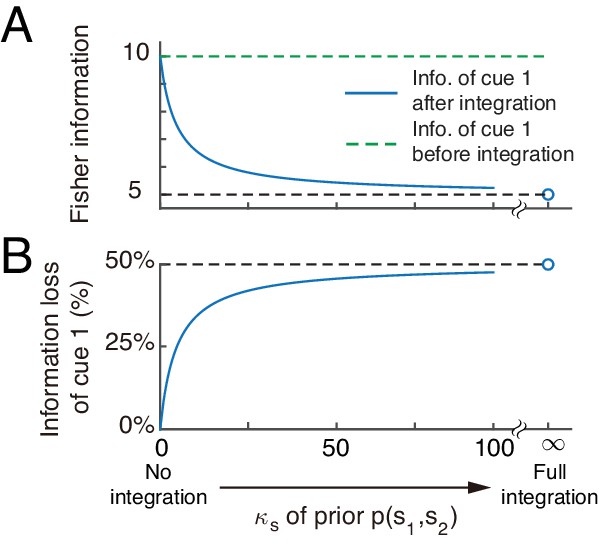
Cue disparity information is lost after integration.

(A) Cue information is lost after integration. The information of cue 1 decreases with the extent of integration, which is controlled by $κ_{s}$ , measuring the correlation between $s_{1}$ and $s_{2}$ . (B) The percentage of cue information loss increases with the extent of integration.

https://doi.org/10.7554/eLife.43753.003

Figure 2

Download asset Open asset

Congruent and opposite neurons in MSTd.

Similar results were found in VIP (Chen et al., 2011). (A–B) Tuning curves of a congruent neuron (A) and an opposite neuron (B). The preferred visual and vestibular directions are similar in (A) but are nearly opposite by 180° in (B). (C) The histogram of neurons according to their difference between preferred visual and vestibular directions. Congruent and opposite neurons are comparable in numbers. (A–B) are adapted from Gu et al. (2008), (C) from Gu et al. (2006).

https://doi.org/10.7554/eLife.43753.004

Figure 3

Download asset Open asset

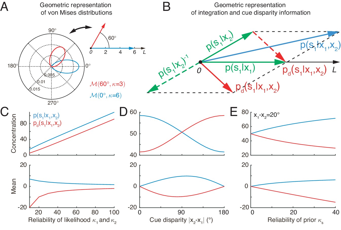
Geometric interpretation of multisensory processing of circular variables.

(A) Two von Mises distributions plotted in the polar coordinate (bottom-left) and their corresponding geometric representations (top-right). A von Mises distribution can be represented as a vector, with its mean and concentration corresponding to the angle and length of the vector, respectively. (B) Geometric interpretation of cue integration and the cue disparity information. The posteriors of $s_{1}$ given single cues are represented by two vectors (green). Cue integration (blue) is the sum of the two vectors (green), and the cue disparity information (red) is the difference of the two vectors. (C–E) The mean and concentration of the integration (blue) and the cue disparity information (red) as a function of the cue reliability (C), cue disparity (D), and reliability of prior (E). In all plots, $κ_{s} = 50$ , $κ_{1} = κ_{2} = 50$ , $x_{1} = 0^{\circ}$ and $x_{2} = 20^{\circ}$ , except that the variables are $κ_{1} = κ_{2}$ in C, $x_{2}$ in D, and $κ_{s}$ in E.

https://doi.org/10.7554/eLife.43753.005

Figure 4

Download asset Open asset

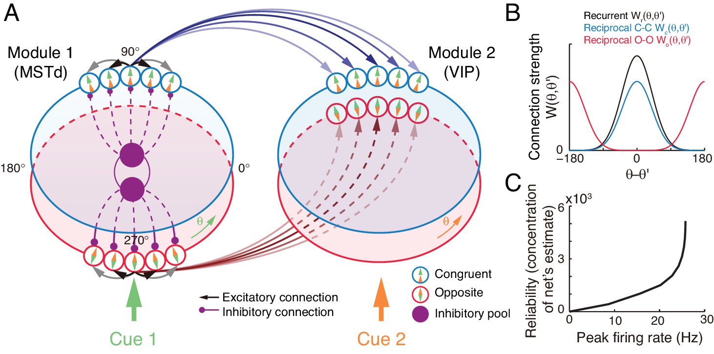
The decentralized neural circuit model for multisensory processing.

(A) The network consists of two modules, which can be regarded as MSTd and VIP respectively. Each module has two groups of excitatory neurons, congruent (blue circles) and opposite neurons (red circles). Each group of excitatory neurons are connected recurrently with each other, and they are all connected to an inhibitory neuron pool (purple disk) to form a continuous attractor neural network. Each module receives a direct cue through feedforward inputs. Between modules, congruent neurons are connected in the congruent manner (blue arrows), while opposite neurons are connected in the opposite manner (brown lines). (B) Connection profiles between neurons. Black line is the recurrent connection pattern between neurons of the same type in the same module. Blue and red lines are the reciprocal connection patterns between congruent and opposite neurons across modules respectively. (C) The reliability of the network's estimate of a stimulus is encoded in the peak firing rate of the neuronal population. Typical parameters of network model: $ω = 3 \times 10^{- 4}$ , $J_{i n t} = 0.5$ , $J_{r c} = 0.3 J_{c}$ , $J_{r p} = 0.5 J_{r c}$ , $I_{b}$ and $F$ in Equation 22 are 1 and 0.5 respectively.

https://doi.org/10.7554/eLife.43753.006

Figure 5

Download asset Open asset

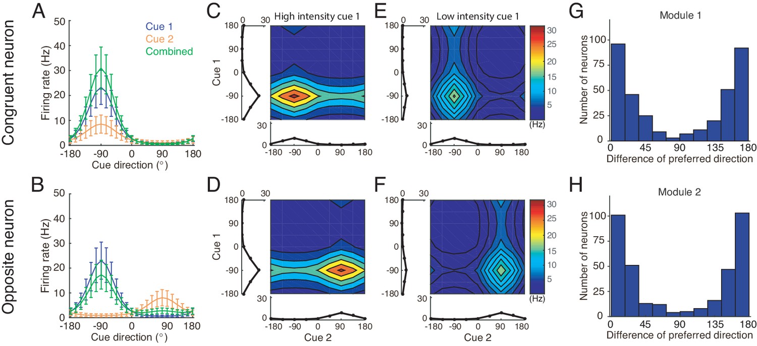
Tuning properties of congruent and opposite neurons in the network model.

(A–B) The tuning curves of an example congruent neuron (A) and an example opposite neuron (B) in module 1 under three cueing conditions. (C–D) The bimodal tuning properties of the example congruent (C) and the example opposite (D) neurons when cue 1 has relatively higher reliability than cue 2 in driving neurons in module 1, with $α_{1} = 0.58 α_{2}$ , where $α_{m}$ is the amplitude of cue m given by Equation 22. The two marginal curves around each contour plot are the unimodal tuning curves. (E–F) Same as (C–D), but cue 1 has a reduced reliability with $α_{1} = 0.12 α_{2}$ . (G–H) The histogram of the differences of neuronal preferred directions with respect to two cues in module 1 (G) and module 2 (H), when the reciprocal connections across network modules contain random components of roughly the same order as the connections. Parameters: (A–B) $α_{1} = 0.35 U_{0}$ , and $α_{2} = 0.8 U_{0}$ ; (C–F) $α_{2} = 1.5 U_{0}$ in (C–D) while $α_{1} = 0.1 U_{0}$ in (E–F). Other parameters are the same as those in Figure 4.

https://doi.org/10.7554/eLife.43753.007

Figure 6 with 2 supplements

Download asset Open asset

Optimal cue integration and segregation collectively emerge in the neural population activities in the network model.

(A) Illustration of the population response of congruent neurons in module 1 when both cues are presented. Color indicates firing rate. Right panel is the temporal average firing rates of the neural population during cue presentation, with shaded region indicating the standard deviation (SD). Note that the neuron index $θ$ refers to the preferred direction with respect to the direct cue conveyed by feedforward inputs. (B) The position of the population activity bump at each instance is interpreted as the network’s estimate of the stimulus, referred to as $z_{1}$ , which is decoded by using population vector. Right panel is the distribution of the decoded network’s estimate during cue presentation. (C–E) The temporal average population activities of congruent (blue) and opposite (red) neurons in module 1 (top row) and module 2 (bottom row) under three cueing conditions: only cue 1 is presented (C), only cue 2 is presented (D), and both cues are simultaneously presented (E). (F–I) Comparing the estimates from congruent and opposite neurons in module 1 with the theoretical predictions, with varying cue intensity (F), with varying cue disparity (G), and with varying reciprocal connection strength between modules (H and I). Symbols: network results; lines: theoretical prediction. The theoretical predictions for the estimates of congruent and opposite neurons are obtained by Equations 4 and 7. Parameters: (A–E) $α_{1} = α_{2} = 0.35 U_{0}$ ; (F) $α_{2} = 0.7 U_{0}$ ; (G–I) $α_{1} = α_{2} = 0.7 U_{0}$ , and others are the same as those in Figure 4. In (F–H), $x_{1} = 0^{\circ}$ , $x_{2} = 20^{\circ}$ and in (I), $x_{1} = 0^{\circ}$ , $x_{2} = 160^{\circ}$ .

https://doi.org/10.7554/eLife.43753.008

Figure 6—figure supplement 1

Download asset Open asset

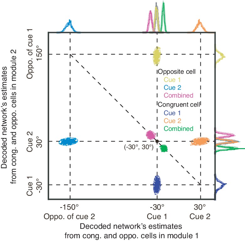
Illustration of decoded joint distributions from congruent and opposite neurons.

Illustration of decoded joint distributions from congruent and opposite neurons respectively in two network modules under three cueing conditions, with the marginal distributions plotted in the margin plot. The joint distribution from congruent neurons in two network modules encode the posterior $p (s_{1}, s_{2} | x_{1}, x_{2})$ , while the one from opposite neurons in two modules represent the cue disparity information $p_{d} (s_{1}, s_{2} | x_{1}, x_{2})$ . Color denotes the cueing condition and type of neurons (see the legend for details). Parameters are the same as those in Figure 6A–E in main text.

https://doi.org/10.7554/eLife.43753.009

Figure 6—figure supplement 2

Download asset Open asset

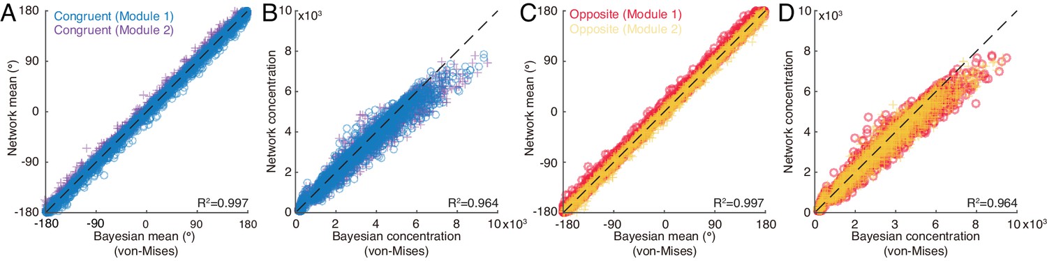
Test of network’s performance.

Comparison of the mean and concentration of network’s estimate with theoretical prediction. (A-B) The mean (A) and the concentration (B) of the congruent neurons in two network modules versus the theoretical prediction. (C-D) The same as (A-B) but for opposite neurons. Parameters: $J_{r c} \in [0.3, 0.4] J_{c}$ , $J_{r p} \in [0.1, 0.7] J_{r c}$ , $α_{1}, α_{2} \in [0.1, 1.5] U_{0}$ , $J_{i n t} \in {0.05, 0.25, 0.5}$ , $x_{1}$ and $x_{2}$ are both uniformly distributed in (−180°, 180°], and others are the same as those in Figure 4 in main text.

https://doi.org/10.7554/eLife.43753.010

Figure 7

Download asset Open asset

Concurrent multisensory processing with congruent and opposite neurons.

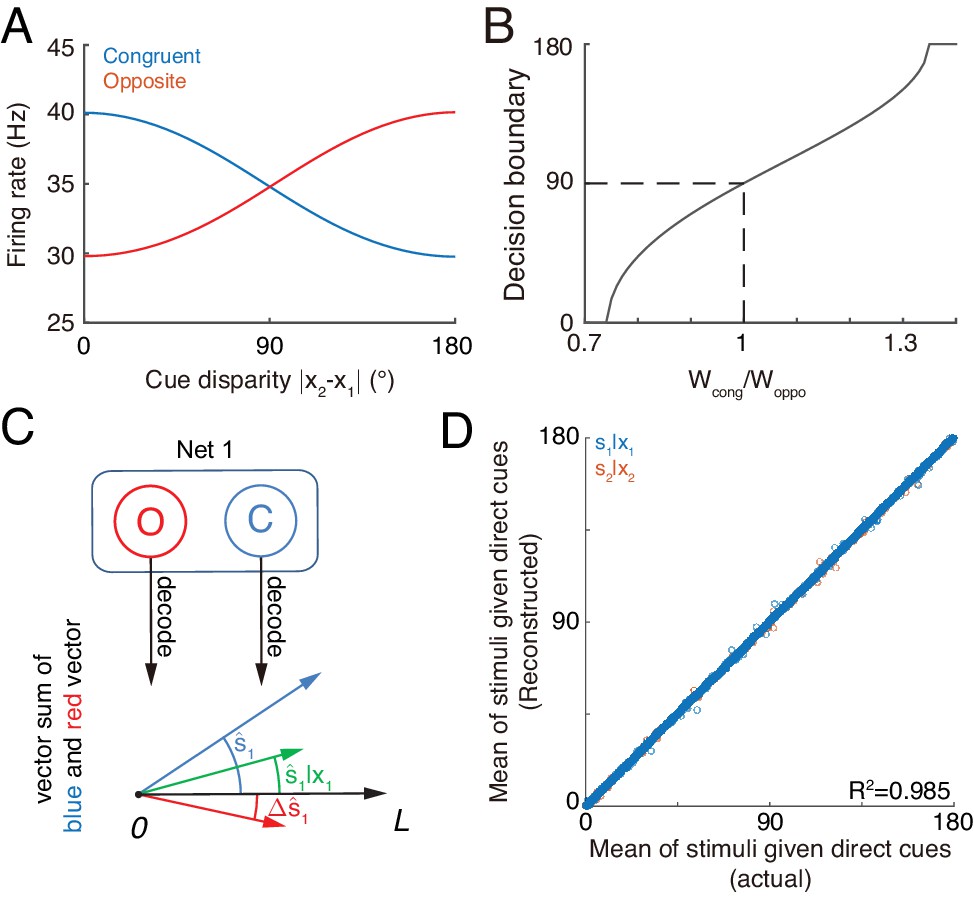
(A–B) Accessing integration versus segregation through the joint activity of congruent and opposite neurons. (A) The firing rate of congruent and opposite neurons exhibit complementary changes with cue disparity $x_{1} - x_{2}$ . (B) The decision boundary of the competition between congruent and opposite neurons changes with read out weight from congruent $W_{c o n g}$ and opposite neurons $W_{o p p o}$ . It is given by the value of $x_{1} - x_{2}$ at which $W_{c o n g} r_{m}^{c} = W_{o p p o} r_{m}^{o}$ . Dashed line is when $W_{c o n g} = W_{o p p o}$ , the decision boundary is at 90°. (C–D) Recovering single cue information from two types of neurons. (C) Illustration of recovering through the joint activities of congruent (blue) and opposite (red) neurons under the combined cue condition. We decoded the estimate from congruent and opposite neurons respectively, and then vector sum the decoded results recovering the single cue information. (D) Comparing the recovered mean of the stimulus given the direct cue with the actual value. Parameters: those in (A–B) are the same as those in Figure 6A, and those in D are the same as those in Figure 6—figure supplement 2.

https://doi.org/10.7554/eLife.43753.011

Figure 8 with 1 supplement

Download asset Open asset

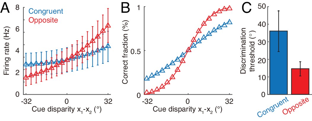
Discrimination of cue disparity by single neurons.

(A) The tuning curve of an example congruent (blue) and opposite (red) neuron with respect to cue disparity $x_{1} - x_{2}$ . In the tuning with respect to cue disparity, the mean of two cues was always at 0°, that is $x_{1} + x_{2} = 0$ , while their disparity $x_{1} - x_{2}$ was varied from −32° to 32° with a step of 4°. The two example neurons are in network module 1, and both prefer 90° with respect to cue 1. However, the congruent neuron prefers 90° of cue 2, while the opposite neuron prefers −90° with respect to cue 2. Error bar indicates the SD of firing rate across trials. (B) The neurometric function of the example congruent and opposite neuron in a discrimination task to determine whether the cue disparity $x_{1} - x_{2}$ is larger than 0° or not. Lines are the cumulative Gaussian fit of the neurometric function. (C) Averaged neuronal discrimination thresholds of the example congruent and opposite neurons. Parameters: $α_{1} = 0.25 U_{0}$ , $α_{2} = 0.8 U_{0}$ , and others are the same as those in Figure 4.

https://doi.org/10.7554/eLife.43753.012

Figure 8—figure supplement 1

Download asset Open asset

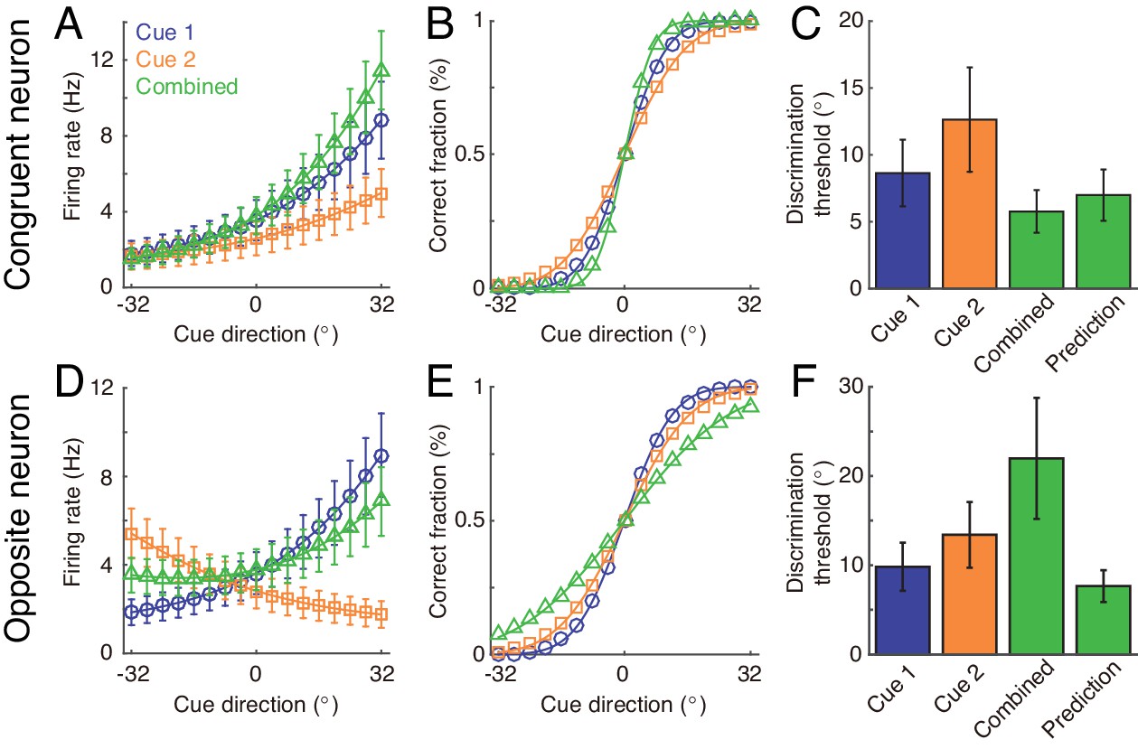
Discrimination of heading direction by single neurons.

Discrimination of heading direction by single neurons. The directions of the two cues are always the same. (A and D) The tuning curve of the example congruent (A) and opposite (D) neurons with cue direction under three cueing conditions. The example neurons are the same as the ones shown in Figure 8 in main text. (B and E) The neurometric function of the example congruent (B) and opposite (E) neurons under three cueing conditions. Smooth lines show the cumulative Gaussian fit of the neurometric functions. (C and F) Average neuronal discrimination thresholds of the example neuron in three cueing conditions compared with the theoretical prediction. Parameters are the same as those in Figure 8 in the main text.

https://doi.org/10.7554/eLife.43753.013

Additional files

Transparent reporting form: https://doi.org/10.7554/eLife.43753.014
Download elife-43753-transrepform-v2.pdf

Download links

A two-part list of links to download the article, or parts of the article, in various formats.

Downloads (link to download the article as PDF)

Open citations (links to open the citations from this article in various online reference manager services)

Mendeley

Cite this article (links to download the citations from this article in formats compatible with various reference manager tools)

Wen-Hao Zhang
He Wang
Aihua Chen
Yong Gu
Tai Sing Lee
KY Michael Wong
Si Wu

(2019)

Complementary congruent and opposite neurons achieve concurrent multisensory integration and segregation

eLife 8:e43753.

https://doi.org/10.7554/eLife.43753

Sign up for email alerts

Privacy notice