Figures and data in A statistical framework to assess cross-frequency coupling while accounting for confounding analysis effects | eLife

Figures
Additional files

13 figures and 1 additional file

Figures

Figure 1

Download asset Open asset

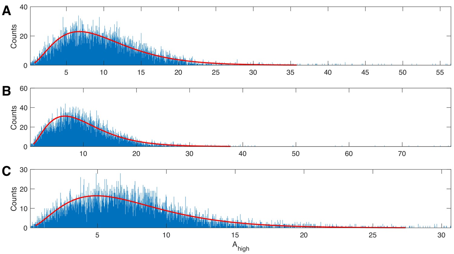
The gamma distribution provides a good fit to example human data.

Three examples of 20 s duration recorded from a single electrode during a human seizure. In each case, the gamma fit (red curve) provides an acceptable fit to the empirical distributions of the high frequency amplitude.

https://doi.org/10.7554/eLife.44287.002

Figure 2

Download asset Open asset

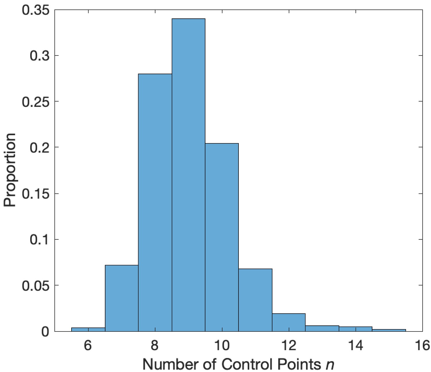
Distribution of the number of control points $(n)$ that minimize the AIC.

Values of $n$ between 7 and 12 minimize the AIC in a simulation with phase-amplitude coupling and amplitude-amplitude coupling.

https://doi.org/10.7554/eLife.44287.003

Figure 3

Download asset Open asset

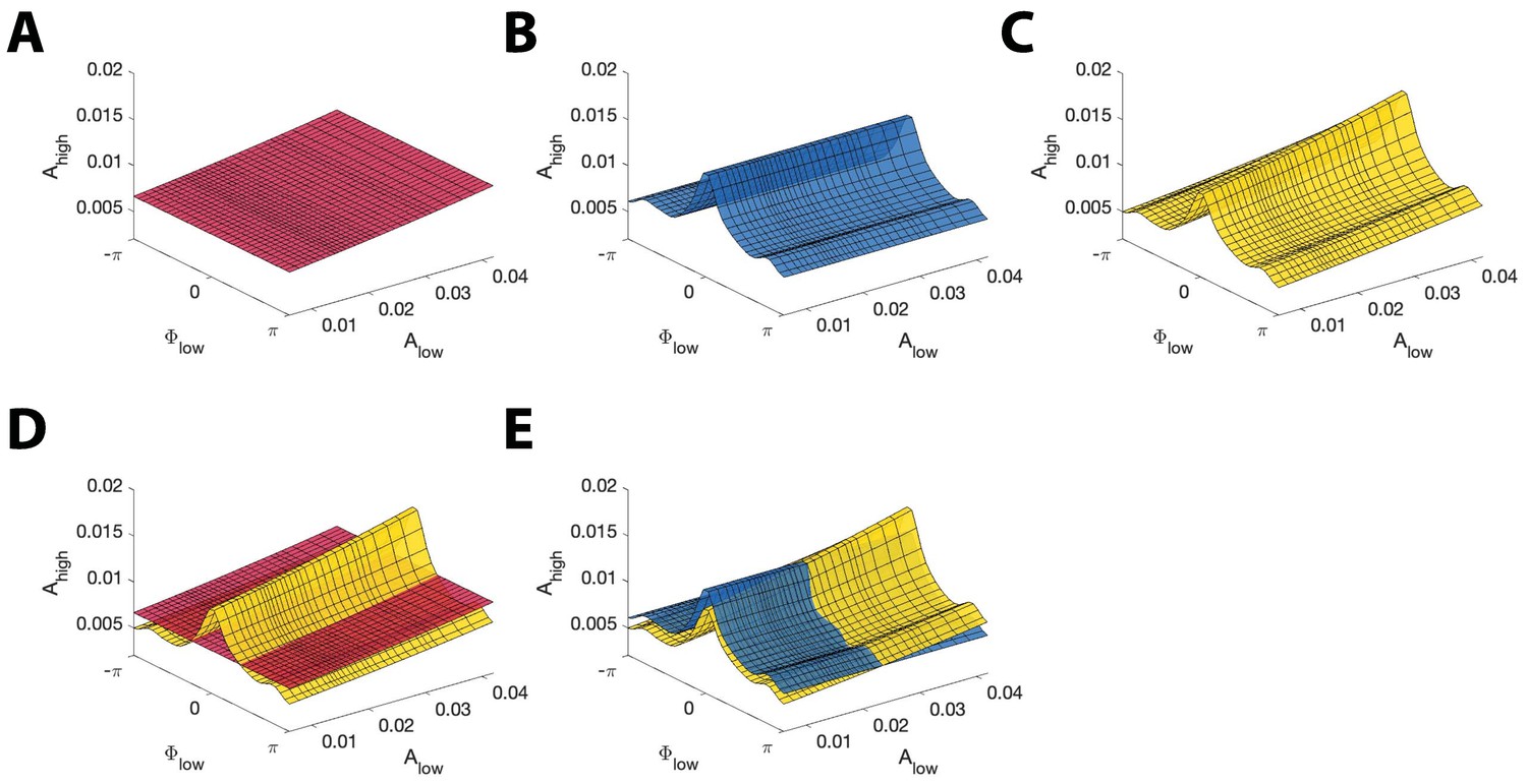
Example model surfaces used to determine $R_{P A C}$ and $R_{A A C}$ .

(A,B,C) Three example surfaces (A) $S_{A_{l o w}}$ , (B) $S_{ϕ_{l o w}}$ , and (C) $S_{A_{l o w}, ϕ_{l o w}}$ in the three-dimensional space ( $A_{l o w}$ , $ϕ_{l o w}$ , $A_{h i g h}$ ). (D) The maximal distance between the surfaces $S_{A_{l o w}}$ (red) and $S_{A_{l o w}, ϕ_{l o w}}$ (yellow) is used to compute $R_{P A C}$ . (E) The maximal distance between the surfaces $S_{ϕ_{l o w}}$ (blue) and $S_{A_{l o w}, ϕ_{l o w}}$ (yellow) is used to compute $R_{A A C}$ .

https://doi.org/10.7554/eLife.44287.004

Figure 4

Download asset Open asset

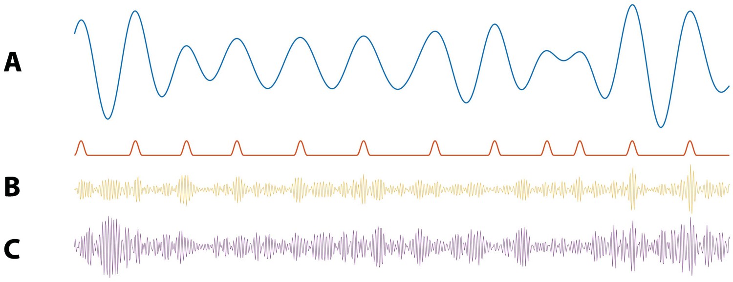
Illustration of synthetic time series with PAC and AAC.

(A) Example simulation of $V_{l o w}$ (blue) and modulation signal M (red). When the phase of $V_{l o w}$ is near 0 radians, M increases. (B) Example simulation of PAC. When the phase of $V_{l o w}$ is approximately 0 radians, the high frequency amplitude (yellow) increases. (C) Example simulations of AAC. When the amplitude of $V_{l o w}$ is large, so is the amplitude of the high frequency signal (purple).

https://doi.org/10.7554/eLife.44287.005

Figure 5

Download asset Open asset

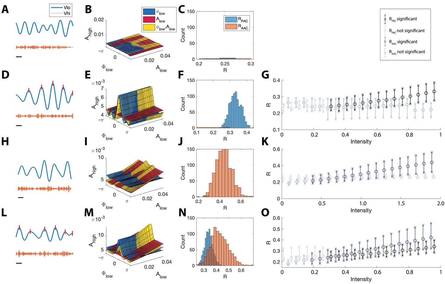
The statistical modeling framework successfully detects different types of cross-frequency coupling.

(A–C) Simulations with no CFC. (A) When no CFC occurs, the low frequency signal (blue) and high frequency signal (orange) evolve independently. (B) The surfaces $S_{A_{low}}$ , $S_{ϕ_{low}}$ , and $S_{A_{low}, ϕ_{low}}$ suggest no dependence of $A_{high}$ on $ϕ_{low}$ or $A_{low}$ . (C) Significant ( $p$ <0.05) values of $𝐑_{PAC}$ and $𝐑_{AAC}$ from 1000 simulations. Very few significant values for the statistics R are detected. (D–G) Simulations with PAC only. (D) When the phase of the low frequency signal is near 0 radians (red tick marks), the amplitude of the high frequency signal increases. (E) The surfaces $S_{A_{low}}$ , $S_{ϕ_{low}}$ , and $S_{A_{low}, ϕ_{low}}$ suggest dependence of $A_{high}$ on $ϕ_{low}$ . (F) In 1000 simulations, significant values of $R_{PAC}$ frequently appear, while significant values of $𝐑_{AAC}$ rarely appear. (G) As the intensity of PAC increases, so do the significant values of $𝐑_{PAC}$ (black), while any significant values of $𝐑_{AAC}$ remain small. (H–K) Simulations with AAC only. (H) The amplitudes of the high frequency signal and low frequency signal are positively correlated. (I) The surfaces $S_{A_{low}}$ , $S_{ϕ_{low}}$ , and $S_{A_{low}, ϕ_{low}}$ suggest dependence of $A_{high}$ on $A_{low}$ . (J) In 1000 simulations, significant values of $𝐑_{AAC}$ frequently appear. (K) As the intensity of AAC increases, so do the significant values of $𝐑_{AAC}$ (blue), while any significant values of $𝐑_{PAC}$ remain small. (L–O) Simulations with PAC and AAC. (L) The amplitude of the high frequency signal increases when the phase of the low frequency signal is near 0 radians and the amplitude of the low frequency signal is large. (M) The surfaces $S_{A_{low}}$ , $S_{ϕ_{low}}$ , and $S_{A_{low}, ϕ_{low}}$ suggest dependence of $A_{high}$ on $ϕ_{low}$ and $A_{low}$ . (N) In 1000 simulations, significant values of $𝐑_{PAC}$ and $𝐑_{AAC}$ frequently appear. (O) As the intensity of PAC and AAC increase, so do the significant values of $𝐑_{PAC}$ and $𝐑_{AAC}$ . In (G,K,O), circles indicate the median, and x’s the 5th and 95th quantiles.

https://doi.org/10.7554/eLife.44287.006

Figure 6

Download asset Open asset

The two measures of PAC increase with intensities near zero.

The mean (circles) and 5^th to 95^th quantiles (x’s) of (A) $𝐑_{PAC}$ and (B) MI for intensity values between 0 and 0.5. Black bars indicate $p_{PAC}$ or $p_{MI}$ is below 0.05 for ≥95% of simulations; gray bars indicate $p_{PAC}$ is not below 0.05 for ≥95% of simulations. While both measures increase with intensity, MI detects more instances of significant PAC than does $𝐑_{PAC}$ for very small values of $I_{PAC}$ .

https://doi.org/10.7554/eLife.44287.007

Figure 7

Download asset Open asset

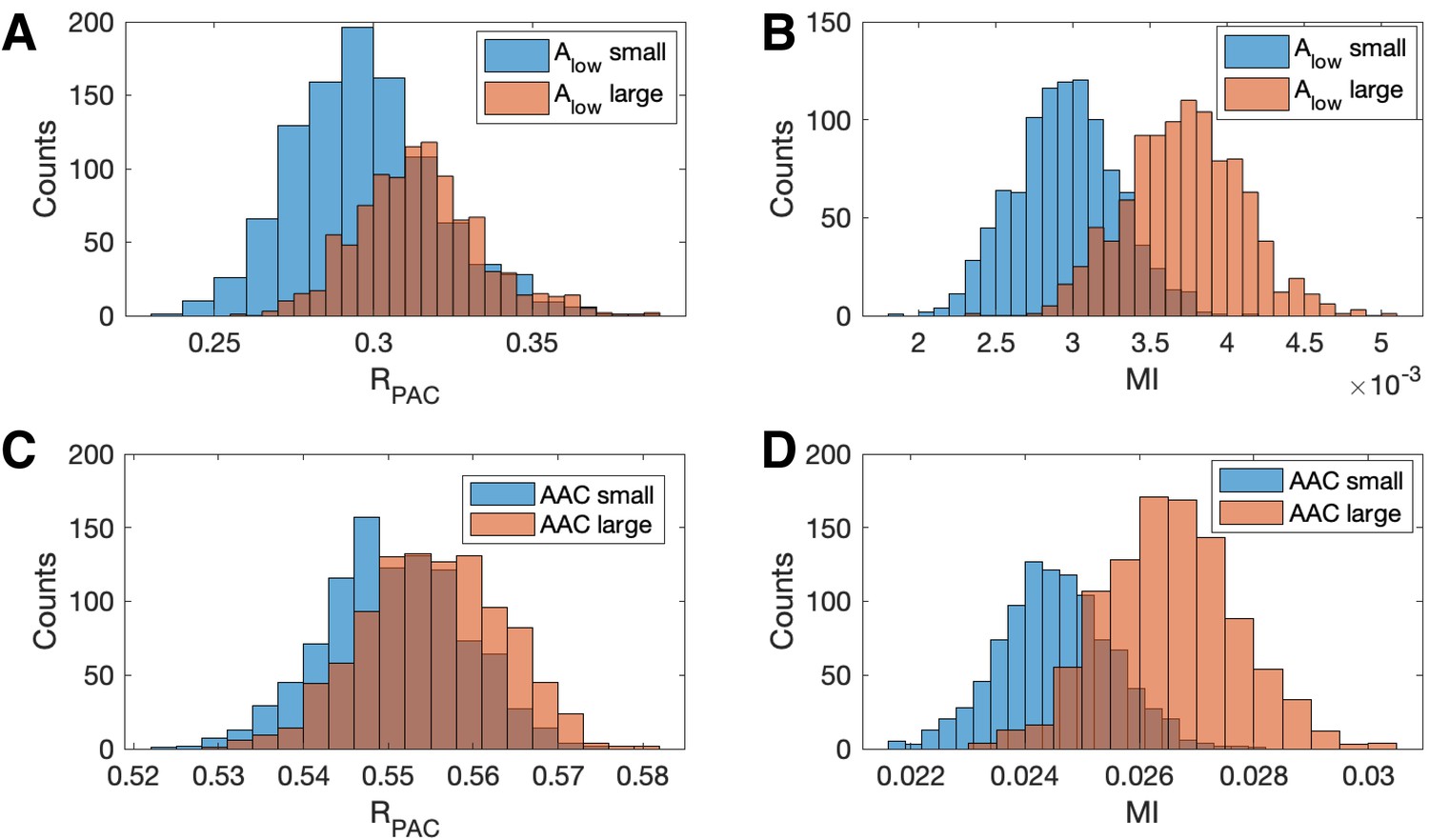
Increases in the amplitude of the low frequency signal, and the amplitude-amplitude coupling (AAC), increase the modulation index more than $R_{P A C}$ .

(A,B) Distributions of (A) $R_{P A C}$ and (B) MI when $A_{l o w}$ is small (blue) and when $A_{l o w}$ is large (red). (C,D) Distributions of (C) $R_{P A C}$ and (D) MI when AAC is small (blue) and when AAC is large (red).

https://doi.org/10.7554/eLife.44287.008

Figure 8

Download asset Open asset

PAC events restricted to a subset of occurrences are still detectable.

(A) The low frequency signal (blue), amplitude envelope (yellow), and threshold (black dashed). (B–C) The modulation signal increases (B) at every occurrence of $ϕ_{l o w} = 0$ , or (C) only when $A_{l o w}$ exceeds the threshold and $ϕ_{l o w} = 0$ .

https://doi.org/10.7554/eLife.44287.009

Figure 9

Download asset Open asset

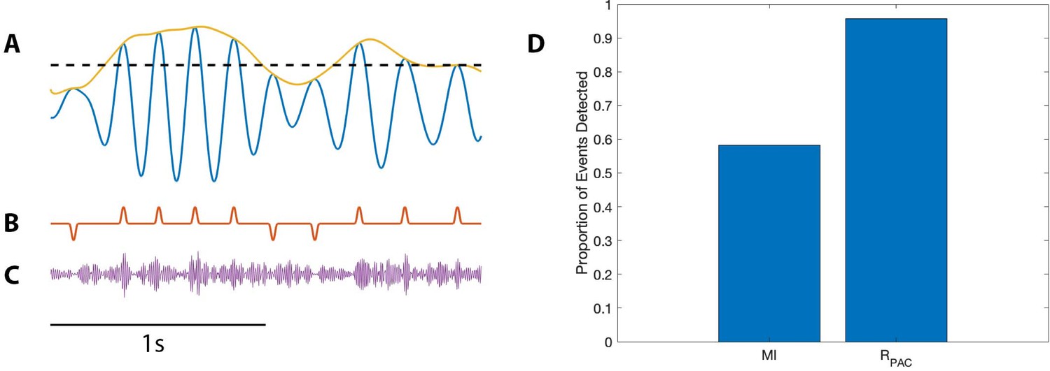
PAC with AAC is accurately detected with the proposed method, but not with the modulation index.

(A) The low frequency signal (blue), amplitude envelope (yellow), and threshold (black dashed). (B) The modulation signal (red) increases when $ϕ_{l o w} = 0$ and $A_{l o w} > T$ , and deceases when $ϕ_{l o w} = 0$ and $A_{l o w} < T$ . (C) The modulated $A_{h i g h}$ signal (purple) increases and decreases with the modulation signal. (D) The proportion of significant detections (out of 1000) for MI and $R_{P A C}$ .

https://doi.org/10.7554/eLife.44287.010

Figure 10

Download asset Open asset

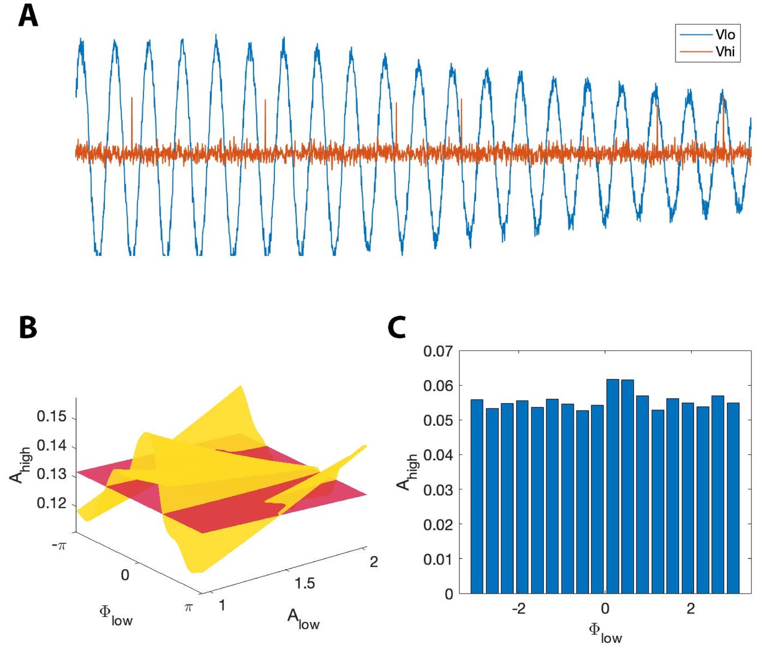
$R_{P A C}$ , but not MI, detects phase-amplitude coupling in a simple stochastic spiking neuron model.

(A) The phase and amplitude of the low frequency signal (blue) modulate the probability of a high frequency spike (orange). (B) The surfaces $S_{A_{l o w}}$ (red) and $S_{A_{l o w}, ϕ_{l o w}}$ (yellow). The phase of maximal $A_{h i g h}$ modulation depends on $A_{l o w}$ . (C) The modulation index fails to detect this type of PAC.

https://doi.org/10.7554/eLife.44287.011

Figure 11

Download asset Open asset

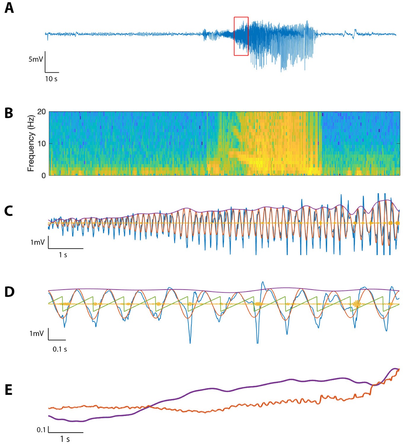
The proposed method detects cross-frequency coupling in an in vivo human recording.

(A,B) Voltage recording (A) and spectrogram (B) from one MEA electrode over the course of a seizure; PAC and AAC were computed for the time segment outlined in red. (C) The 10 s voltage trace (blue) corresponding to the outlined segment in (A), and $V_{low}$ (red), $V_{high}$ (yellow), and $A_{low}$ (purple). (D) A 2 s subinterval of the voltage trace (blue), $V_{low}$ (red), $V_{h i g h}$ (yellow), $A_{l o w}$ (purple), and $ϕ_{l o w}$ (green). (E) $A_{l o w}$ (purple) and $A_{h i g h}$ (red) for the 10 s segment in (C), normalized and smoothed.

https://doi.org/10.7554/eLife.44287.012

Figure 12

Download asset Open asset

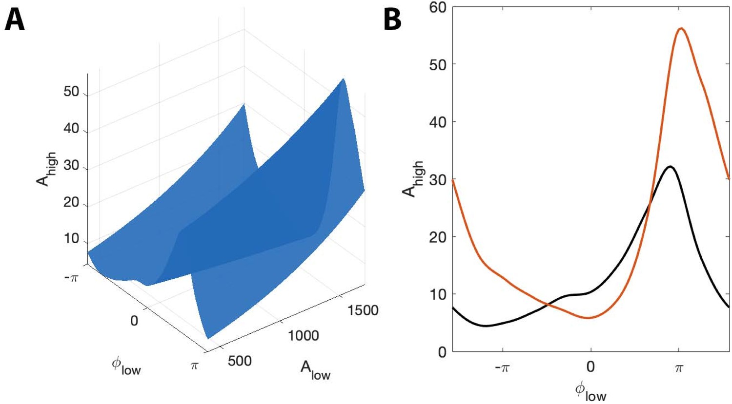
The $S_{A_{low}, ϕ_{low}}$ surface shows how PAC changes with the low frequency amplitude and phase during an interval of human seizure.

(A) The full model surface (blue) in the ( $ϕ_{l o w}$ , $A_{l o w}$ , $A_{h i g h}$ ) space, and components of that surface when (B) $A_{l o w}$ is small (black), and $A_{l o w}$ is large (red).

https://doi.org/10.7554/eLife.44287.013

Figure 13

Download asset Open asset

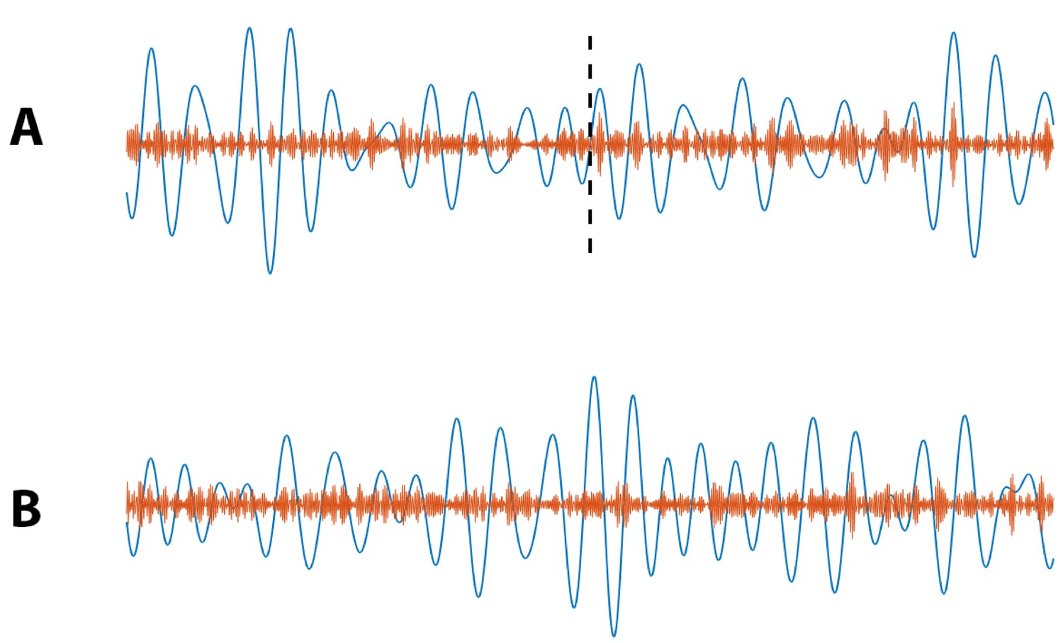
Example simulated $V_{low}$ (blue) and $V_{high}$ (orange) signals for which (A) PAC increases at 20 s (indicated by black dashed line), and (B) no increase in PAC occurs.
https://doi.org/10.7554/eLife.44287.014

Additional files

Transparent reporting form: https://doi.org/10.7554/eLife.44287.015
Download elife-44287-transrepform-v2.docx

Download links

A two-part list of links to download the article, or parts of the article, in various formats.

Downloads (link to download the article as PDF)

Article PDF

Open citations (links to open the citations from this article in various online reference manager services)

Mendeley

Cite this article (links to download the citations from this article in formats compatible with various reference manager tools)

Jessica K Nadalin
Louis-Emmanuel Martinet
Ethan B Blackwood
Meng-Chen Lo
Alik S Widge
Sydney S Cash
Uri T Eden
Mark A Kramer

(2019)

A statistical framework to assess cross-frequency coupling while accounting for confounding analysis effects

eLife 8:e44287.

https://doi.org/10.7554/eLife.44287

Sign up for email alerts

Privacy notice