Figures and data in Environmental heterogeneity can tip the population genetics of range expansions

Figures
Tables
Additional files

8 figures, 2 tables and 1 additional file

Figures

Figure 1 with 3 supplements

Download asset Open asset

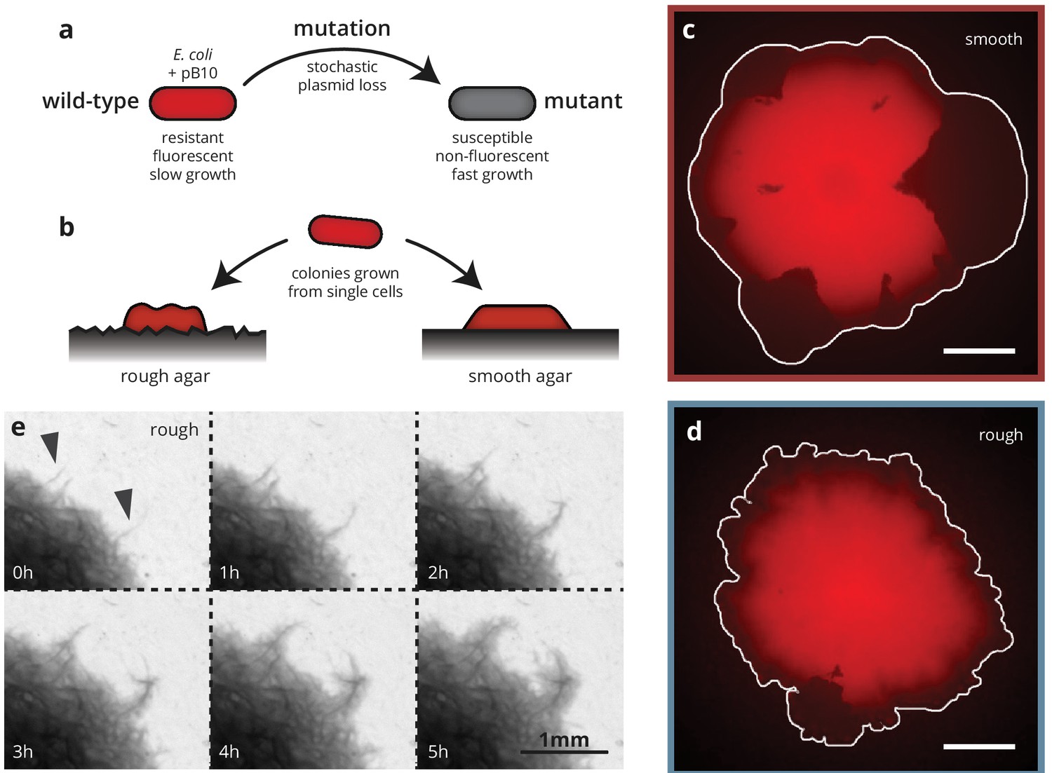
Substrate roughness impacts bacterial colony morphology.

(a and b) Colonies of *E. coli* were grown from single cells harboring a plasmid containing a fluorescence gene and a resistance cassette. Loss of the plasmid leads to non-fluorescent ('mutant’) sectors in the population that expand at the expense of the fluorescent ('wild-type’) population. Colony morphology depends on whether the colony is grown on smooth (c) or rough (d) agar surfaces (Materials and methods). White scale bars are 2 mm. (e) On rough surfaces, troughs in the surface direct growth along them, leading to locally accelerated regions (arrows) that widen slowly and are eventually integrated with the bulk of the population.

https://doi.org/10.7554/eLife.44359.003

Figure 1—figure supplement 1

Download asset Open asset

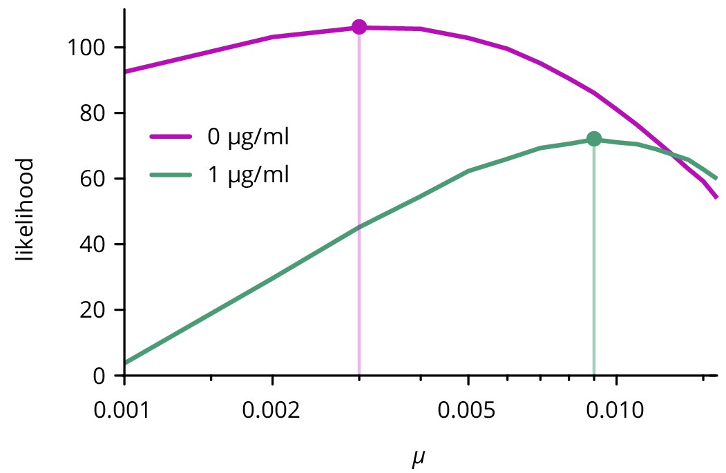
Likelihood of mutation rate for two different concentrations of doxycycline.

Only the curves with the maximum likelihood value for $s$ are shown.

https://doi.org/10.7554/eLife.44359.004

Figure 1—figure supplement 1—source data 1 Source data for Figure 1—figure supplement 1 (Likelihood of mutation rates).: https://doi.org/10.7554/eLife.44359.005
Download elife-44359-fig1-figsupp1-data1-v2.csv

Figure 1—figure supplement 2

Download asset Open asset

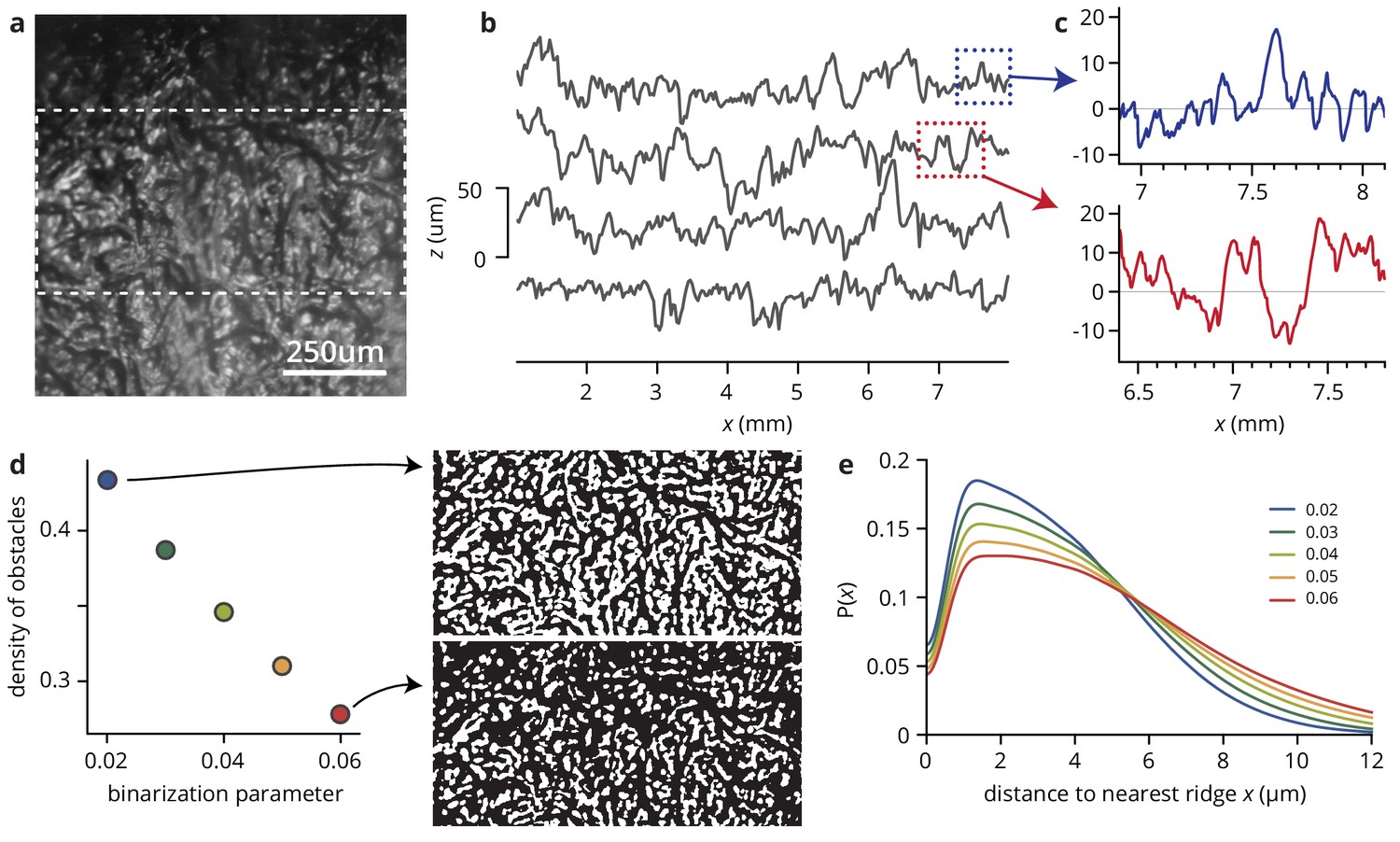
Analysis of substrate roughness.

(a) Microscopic image of an agar surface patterned with filter paper as described in Materials and methods. The image was created by stitching together six images taken on a Dektak 150 profilometer under oblique illumation. Light areas correspond to elevations, dark areas to troughs. (b) Traces along the vertical direction in panel (a), shifted for visibility (see Materials and methods). The mean roughness is 10 ± 1 μm, with a range of elevations to troughs of 50 μm. (c) Close-up of longer runs in (b). (d) Estimating the density of 'obstacles’, that is parts of the patterns that are significantly elevated compared to their surroundings. The images are binarized version of the area between the dashed lines in (a), using the LocalAdaptativeBinarize function in Mathematica with at 15 pixel radius; pixels are scored as one if they are brighter than $0.8 \times μ + 0.05 \times σ + ϵ$ , where $μ$ and $σ$ are the local mean and standard deviation in intensity, and $ϵ$ is an intensity shift. The dependence of the proportion of pixels scored as one on $ϵ$ is shown in the plot in (d). (e) For different values of $ϵ$ , histograms of the distances $x$ of dark pixels from the nearest white pixel, showing that the width of 'valleys’, i.e., the distance between adjacent ridges, is limited to ≤25 μm (twice the range of $x$ ).

https://doi.org/10.7554/eLife.44359.006

Figure 1—figure supplement 2—source data 1 Source data for Figure 1—figure supplement 2 (Five stylus runs to measure substrate roughness).: https://doi.org/10.7554/eLife.44359.007
Download elife-44359-fig1-figsupp2-data1-v2.zip

Figure 1—figure supplement 3

Download asset Open asset

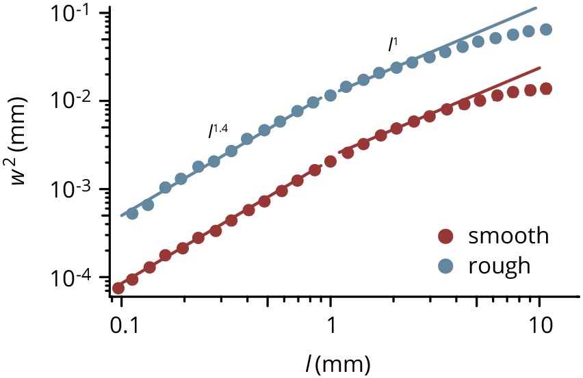
Roughness of *E.coli* colonies on smooth and rough substrates, defined as the mean square deviation from the best-fit circle.

Colony boundaries were extracted and the variance $w^{2}$ of the radius fluctuations measured over different window lengths $l$ . For interfaces in the KPZ universality class, $w^{2} \sim l$ . Points are averages over 118 (smooth) and 193 (rough) colonies, error bars are smaller than the symbols.

https://doi.org/10.7554/eLife.44359.008

Figure 1—figure supplement 3—source data 1 Source data for Figure 1—figure supplement 3 (Roughness of smooth and rough colonies).: https://doi.org/10.7554/eLife.44359.009
Download elife-44359-fig1-figsupp3-data1-v2.csv

Figure 2 with 5 supplements

Download asset Open asset

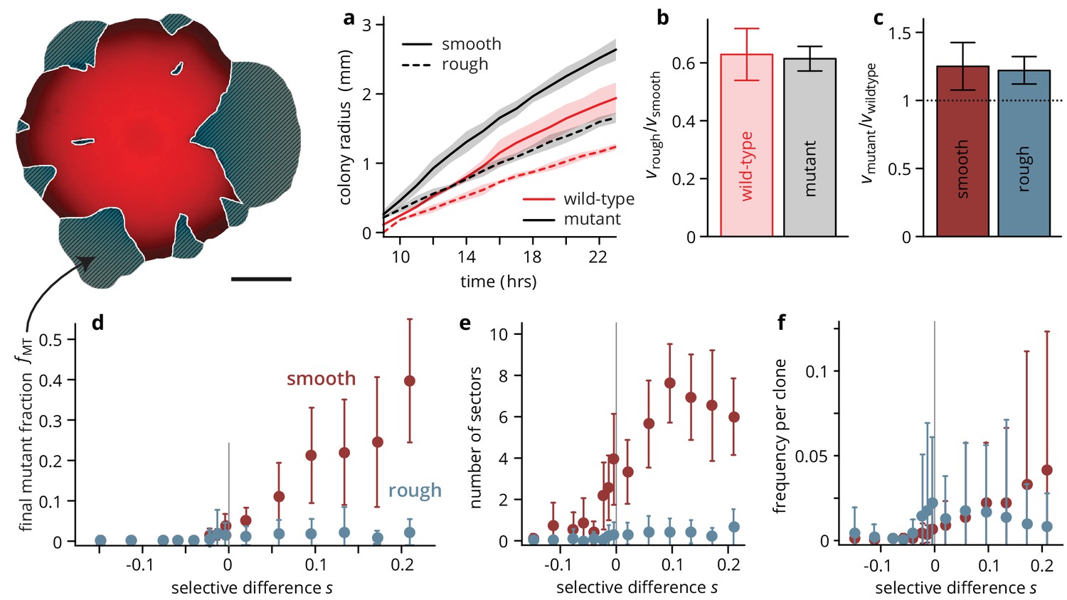
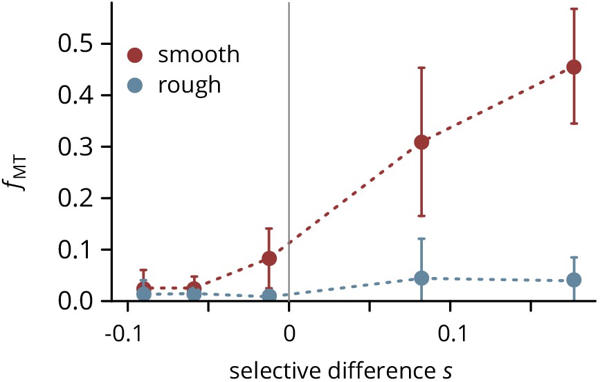
Substrate roughness limits the efficacy of selection in bacterial colonies.

(**a–c**) The roughness of the growth substrate reduces the radial expansion rate but has no impact on the relative growth rates between mutants and wild type (averages over four colonies per condition, shaded areas in panel (a) are ± 1 standard deviation). (d) The final mutant frequency $f_{MT}$ (measured as the area fraction of non-fluorescent clones in the colonies, shown in white outline in sketch above) after 3 days of growth for mutants of a given fitness (dis)advantage $s$ differed strongly depending on the roughness of the surface they were grown on, despite relative growth rate differences $s$ being comparable (c) (throughout, points are averages over colonies, see Table 1, error bars are ± 1 standard deviation). The number of establishing sectors (e) was much smaller in rough colonies, with typically no more than two sectors per colony even for large $s$ . The sizes of individual clones are broadly distributed on both substrates (see also Figure 3), but the mean clone size (f) did not vary as strongly with $s$ in rough colonies as it did in smooth colonies.

https://doi.org/10.7554/eLife.44359.010

Figure 2—source data 1 Source data for Figure 2. colony radii.csv Source data for panel b (colony radii over time). fMT data.csv Source data for panel d (mutant frequency vs selective difference $s$ for rough and smooth substrates). sectors data.csv Source data for panel e (number sectors vs selective difference $s$ for rough and smooth substrates). fClone data.csv Source data for panel f (area fraction of individual clones vs selective difference $s$ for rough and smooth substrates).: https://doi.org/10.7554/eLife.44359.020
Download elife-44359-fig2-data1-v2.zip

Figure 2—figure supplement 1

Download asset Open asset

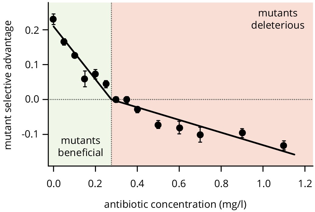
Selective difference between mutants and wild type at different concentrations of doxycycline.

For low antibiotic concentrations, plasmid loss is beneficial such that mutants have an advantage, while the mutants become first neutral and then deleterious for higher concentrations. Points are averages over 12 colony collisions, error bars are standard error of the mean.

https://doi.org/10.7554/eLife.44359.011

Figure 2—figure supplement 1—source data 1 Source data for Figure 2—figure supplement 1 (Fitness measurements at various concentrations of doxycycline).: https://doi.org/10.7554/eLife.44359.012
Download elife-44359-fig2-figsupp1-data1-v2.csv

Figure 2—figure supplement 2

Download asset Open asset

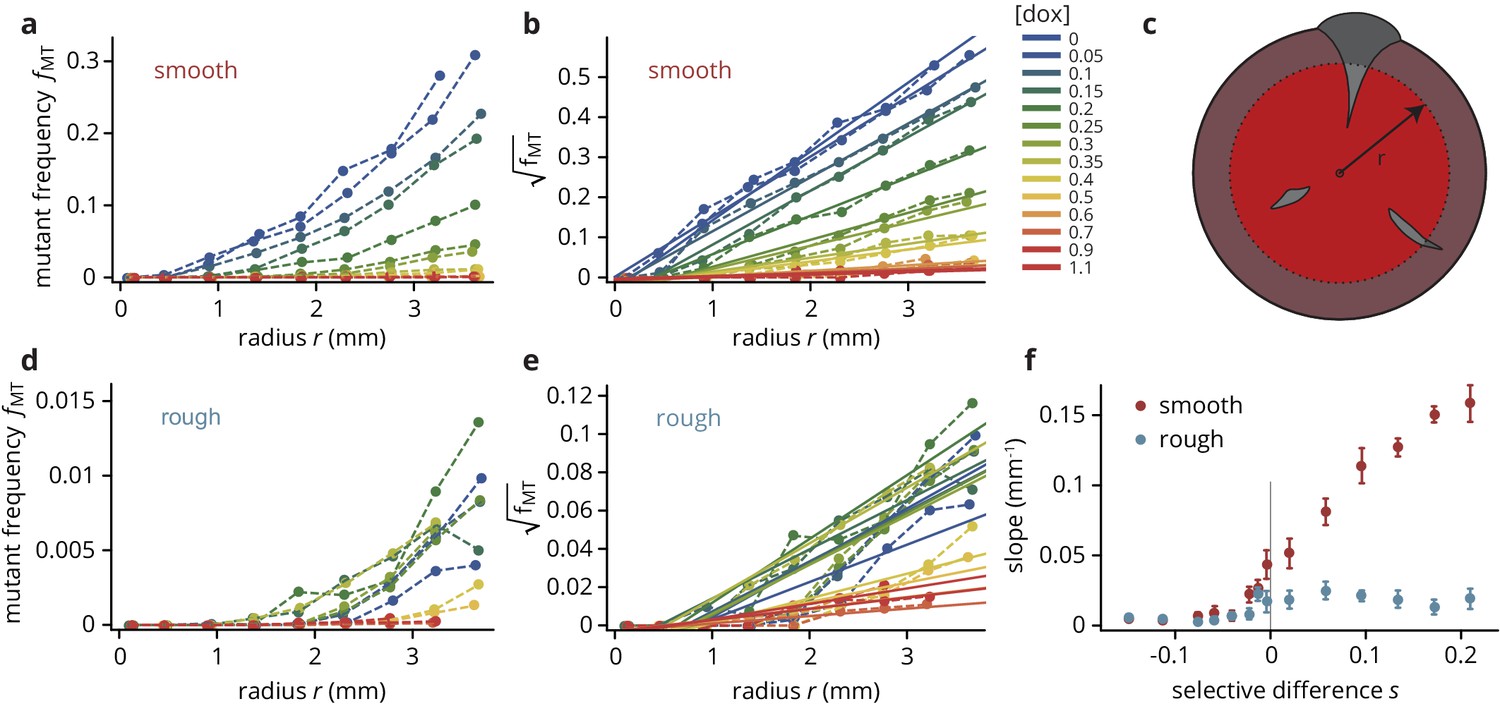
Mutant frequency $f_{MT}$ as a function of radius $r$ (see panel (c) for schematic), for smooth (**a–b**) and rough (**d–e**) colonies.

The traces are approximately quadratic in $r$ , such that we can fit straight lines to the square-root transformed traces whose slopes provide a useful summary observable of the traces, shown in panel (f).

https://doi.org/10.7554/eLife.44359.013

Figure 2—figure supplement 2—source data 1 Source data for Figure 2—figure supplement 2 (Mutant frequency $f_{MT}$ as a function of radius $r$ for smooth and rough colonies).: https://doi.org/10.7554/eLife.44359.014
Download elife-44359-fig2-figsupp2-data1-v2.zip

Figure 2—figure supplement 3

Download asset Open asset

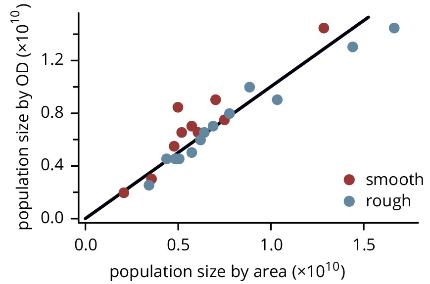
Population size of colonies estimated by measuring colony height and area, and by resuspending and measuring the resulting optical density.

The black line has slope 1. Note that the colonies were chosen to span a wide range of sizes; their sizes are not representative of the overall distribution of colony sizes.

https://doi.org/10.7554/eLife.44359.015

Figure 2—figure supplement 3—source data 1 Source data for Figure 2—figure supplement 3 (Colony sizes on rough and smooth substrates).: https://doi.org/10.7554/eLife.44359.016
Download elife-44359-fig2-figsupp3-data1-v2.csv

Figure 2—figure supplement 4

Download asset Open asset

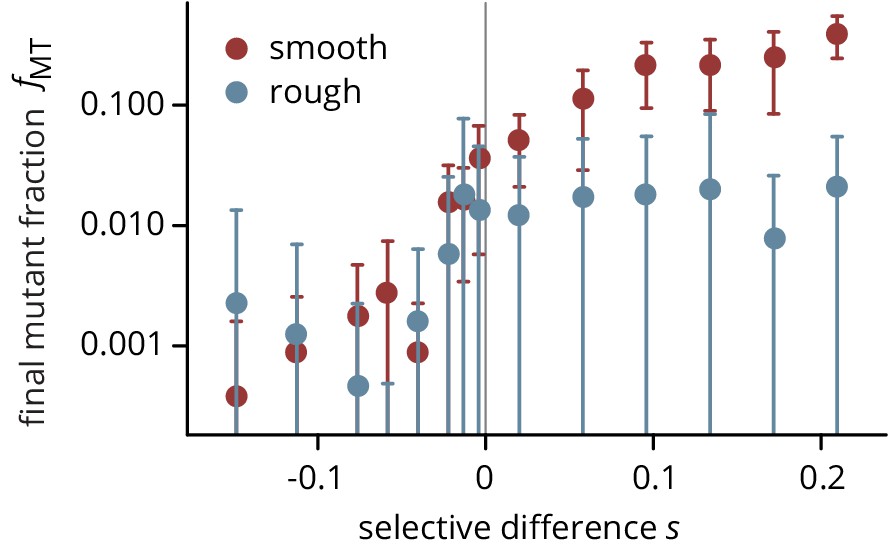
Final frequency of mutants after 3 days of growth, on smooth (red) and rough (blue) plates.

Same data as Figure 2a, plotted on a semi-logarithmic scale.

https://doi.org/10.7554/eLife.44359.017

Figure 2—figure supplement 5

Download asset Open asset

Mutant frequency measured in colonies grown on smooth and rough substrates at five doxycycline concentrations (converted to fitness differences $s$ as described in the main text) in a biological replicate experiment.

Error bars are ± 1 standard deviation.

https://doi.org/10.7554/eLife.44359.018

Figure 2—figure supplement 5—source data 1 Source data for Figure 2—figure supplement 5 (Mutant frequency $f_{MT}$ vs selective difference $s$ in replicate experiment).: https://doi.org/10.7554/eLife.44359.019
Download elife-44359-fig2-figsupp5-data1-v2.csv

Figure 3

Download asset Open asset

Clone size distribution $P (X > x)$ for colonies grown on smooth (a) and rough (b) substrates.

Deleterious mutants are shown in magenta tones; their clones are typically small. Neutral clones are shown in green; their size distribution had a broad tail. Advantageous mutations in smooth colonies were even more broadly distributed, as large sectors establish more often. By contrast, beneficial clones in rough colonies had size distributions that were indistinguishable from the distribution for neutral mutations.

https://doi.org/10.7554/eLife.44359.021

Figure 3—source data 1 Source data for Figure 3. sfs_smooth.csv Source data for panel a (clone size distribution for smooth colonies). sfs rough.csv Source data for panel b (clone size distribution for rough colonies).: https://doi.org/10.7554/eLife.44359.022
Download elife-44359-fig3-data1-v2.zip

Figure 4 with 1 supplement

Download asset Open asset

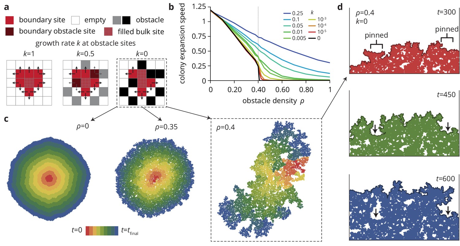
A minimal model captures the change in colony morphology in heterogeneous environments.

(a) The simulation proceeds by allowing cells with empty neighbors ('boundary sites’) to divide into empty space. Disorder sites (gray/black, density $ρ$ ) are randomly distributed over the lattice. (b) As the obstacle transparency, that is the growth rate $k$ at disorder sites, is reduced, the colony expansion speed decreases as a function of the obstacle density. For impassable disorder sites ('obstacles’, $k = 0$ ), the expansion speed vanishes above a critical obstacle density $ρ_{c} \approx 0.4$ , beyond which the population was trapped and could not grow to full size. (c) As $ρ$ approached $ρ_{c}$ colony morphology became increasing fractal. Colors from red to blue show the colony shape at different times. (d) Near the critical obstacle density $ρ_{c} \approx 0.4$ , only few individual sites near the front have empty neighbors, leading to local *pinning* of the front (arrows), where the front can only progress by lateral growth into the pinned region.

https://doi.org/10.7554/eLife.44359.024

Figure 4—source data 1 Source data for Figure 4 (Colony expansion rate in heterogeneous environments).: https://doi.org/10.7554/eLife.44359.027
Download elife-44359-fig4-data1-v2.csv

Figure 4—figure supplement 1

Download asset Open asset

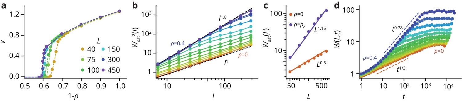
Characterization of Eden clusters with obstacles ( $k = 0$ ).

(a) Taking the front speed $v$ as the order parameter, there is a phase transition at a critical obstacle density $ρ_{c} (L)$ depending on system size $L$ . For an infinite system, $ρ_{c} \approx 0.41 \pm 0.01$ . For $ρ < ρ_{c}$ , we have $v \sim {| ρ - ρ_{c} |}^{0.21}$ . (b) Roughness $W$ of fully developed interfaces at $L = 400$ for varying obstacle densities, as a function of the window length $l$ , such that $W \sim t^{α}$ . At $ρ = 0$ , we find $α = 1 / 2$ , consistent with the KPZ universality class. At $ρ_{c}$ , we find $α_{loc} \approx 0.9$ , consistent with the QEW universality class (see *Theory* in the Materials and methods section), which is known to be characterized by two roughness exponents, a local exponent ( $α_{loc}$ , panel b), and a global exponent $α_{G} \approx 1.15 > α_{loc}$ when the roughness is measured over the whole system size (see panel c) (Amaral et al., 1995). Importantly for $0 < ρ < ρ_{c}$ , there is a crossover length scale below which the system displays QEW scaling, whereas it returns to the KPZ scaling on longer length scales. (d) The time evolution $W (t) \sim t^{β}$ of the interface also follows dynamics consistent with KPZ ( $β = 1 / 3$ ) and QEW ( $β \approx 0.78$ ) in the limiting cases. For intermediate $0 ≪ ρ ≪ ρ_{c}$ , there is a crossover from qEW at short times to KPZ dynamics at longer times, before the roughness saturates at a $ρ$ -dependent value. For easier analysis, all simulations were performed in a box-like geometry.

https://doi.org/10.7554/eLife.44359.025

Figure 4—figure supplement 1—source data 1 Source data for Figure 4—figure supplement 1 (Analysis of colony expansion rate (v(rho).xlsx), interface width as a function of window length (w(l).xslx) and time (w(t).xslx), and saturation width (Wsat.xlsx)).: https://doi.org/10.7554/eLife.44359.026
Download elife-44359-fig4-figsupp1-data1-v2.zip

Figure 5 with 1 supplement

Download asset Open asset

A simple lattice model reproduces strong impact of environmental heterogeneity on evolutionary dynamics.

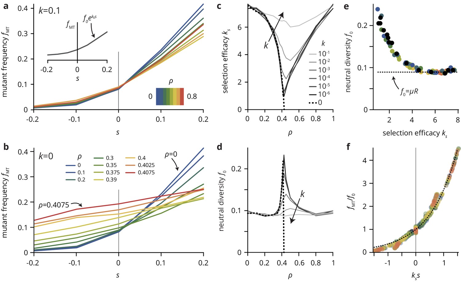
(**a,b**) The mutant frequency $f_{MT}$ as a function of the selective advantage $s$ of the mutants always increases with $s$ to a degree that depends on the density $ρ$ and the transparency $k$ of the disorder sites. (**c,d**) Parametrizing the mutant frequency for various values of $k$ and $ρ$ heuristically with $f_{MT} = f_{0} e^{k_{s} s}$ (panel a, inset), we fit the neutral diversity $f_{0}$ (shown in panel d) and the selection efficacy $k_{s}$ (panel c). The selection efficacy $k_{s}$ serves as an inverse selection scale, describing the dependence of $f_{MT}$ on $s$ . (e) A scatter plot of the fit parameters $f_{0}$ and $k_{s}$ for all values of $k$ and $ρ$ reveals that they are effectively not independent parameters, but that $f_{0}$ entirely determines $k_{s}$ and vice-versa (for a given population size $N$ and mutation rate μ; here, $N = 10^{5}$ and $μ = 0.0005$ ). The dashed line represents the expect neutral diversity for a circular colony, where $f_{0} = μ R$ , with $R = \sqrt{N / π}$ the colony radius (Fusco et al., 2016). (f) Rescaling all curves by fitted values of $k_{s}$ and $f_{0}$ , all points fall close to a master curve given by $e^{k_{s} s}$ (dashed line), motivating the parametrization introduced in (a).

https://doi.org/10.7554/eLife.44359.028

Figure 5—source data 1

Source data for Figure 5.

ks_values.csv. Source data for panel c (fit parameter $k_{s}$ for various parameter values $ρ$ and $k$ ). f0 values.csv Source data for panel d (fit parameter $f_{0}$ for various parameter values $ρ$ and $k$ ). rescaled fMT data.xlsx Source data for panel f (rescaled $f_{MT}$ for various parameter values $ρ$ and $k$ ).: https://doi.org/10.7554/eLife.44359.031
Download elife-44359-fig5-data1-v2.zip

Figure 5—figure supplement 1

Download asset Open asset

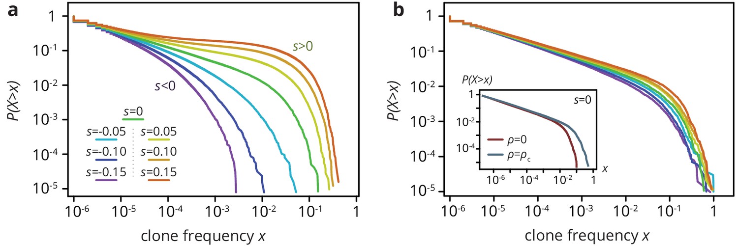
Clone size distribution $P (X > x)$ for colonies grown on smooth (a) and rough (b) substrates in simulations.

Deleterious mutants are shown in magenta tones; their clones are typically small. Neutral clones are shown green; their size distribution is broad. Advantageous mutations (red tones) are even more broadly distributed, as large sectors establish more often. In the absence of environmental heterogeneity, the clone size distribution $P (X > x)$ was very broad, with a low-frequency power-law regime $x^{- 2 / 5}$ corresponding to mutant bubbles and a steeper power-law at high frequencies characterizing sector sizes (Fusco et al., 2016). A deleterious fitness effect $s$ of the mutations created an effective cut-off because sectors no longer formed, whereas positive $s$ increased the likelihood of high-frequency clones, because sectors establish more often and grow to larger frequencies when they do. At the critical obstacle density, we found that a neutral clone size distribution that was remarkably similar to what we found without environmental heterogeneity (b, inset). By contrast, selective differences between mutants and wild type had a much less pronounced effect on the clone size distribution as the density of obstacles increased. The clone size distribution for both beneficial and deleterious mutations thus resembled the distribution for neutral mutations. In simulations at the critical obstacle density $ρ = ρ_{c}$ , $P (X > x)$ became roughly independent of $s$ , such that fitness effects associated with the mutations were effectively inconsequential at the level of individual clones.

https://doi.org/10.7554/eLife.44359.029

Figure 5—figure supplement 1—source data 1 Source data for Figure 5—figure supplement 1 (Clone size distribution for various $s$ for $ρ = 0$ and $ρ = 0.4$ ).: https://doi.org/10.7554/eLife.44359.030
Download elife-44359-fig5-figsupp1-data1-v2.zip

Figure 6 with 1 supplement

Download asset Open asset

Neutral lineage dynamics change with environmental heterogeneity.

Lineage trees extracted from simulated colonies without ( $ρ = 0$ ), (a) and with critical ( $ρ = 0.4$ ), (b) environmental heterogeneity. (c) The lineage structure is characterized by the fluctuations $l_{⟂}$ of the lineages in forward time $t$ , and the pair coalescence time $T_{2}$ (backwards in time) of two samples that are a distance $Δ x$ apart. (d) The lineage fluctuations depend on the environmental heterogeneity: in the absence of environmental disorder, lineage fluctuations scale as $t^{2 / 3}$ , whereas the lineages are rougher in strong disorder, scaling as $t^{0.86}$ . Strong lineage fluctuations in heterogeneous environments also impact the mean pair coalescence time of two samples a distance $Δ x$ apart by allowing lineages from distant regions of the colony to coalesce earlier than without environmental heterogeneity (panel e). As a consequence, the persistence probability $U (T_{2})$ , that is the probability that two sampled lineages have a pair coalescence time greater than $T_{2}$ is typically greater in homogeneous than in heterogeneous environments, even when conditioning on small distance between samples (solid lines, $Δ x < 0.05 Δ x_{m a x}$ ; dashed lines, $Δ x < 0.05 Δ x_{m a x}$ ).

https://doi.org/10.7554/eLife.44359.032

Figure 6—source data 1

Source data for Figure 6.

lineage_fluctuations.csv Source data for panel d (lineage fluctuations $l_{⟂}$ vs forward time $t$ ). T2vsDeltaX data.csv Source data for panel e (mean pair coalescence time $T_{2}$ vs pair distance $Δ x$ ). P(T2) data.csv Source data for panel f (persistence probability $U (T_{2})$ vs pair coalescence time $T_{2}$ ).: https://doi.org/10.7554/eLife.44359.035
Download elife-44359-fig6-data1-v2.zip

Figure 6—figure supplement 1

Download asset Open asset

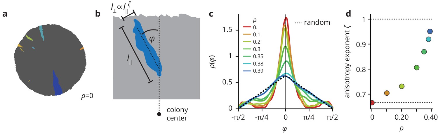
Environmental heterogeneity alters the shapes of mutant clones.

(a) Mutant clones (colored by the time of mutation) in a simulated colony grown in a homogeneous environment. (c) Environmental heterogeneity impacts the directionality of clones (measured by the angle $ϕ$ that a clone’s semi-major axis makes with the radial direction, see panel (b)), which are mostly aligned with the radial direction for smooth colonies, but point in essentially random directions in heterogeneous environments. (d) Clones become more isotropic as the pinning transition is approached, as measured by the anisotropy exponent $ζ$ which quantifies how the typical width $l_{⟂} \sim l_{∥}^{ζ}$ of a clone scales with its length $l_{∥}$ .

https://doi.org/10.7554/eLife.44359.033

Figure 6—figure supplement 1—source data 1 Source data for Figure 6—figure supplement 1 (Clone angles and anisotropy exponents for neutral mutations for various $ρ$ ).: https://doi.org/10.7554/eLife.44359.034
Download elife-44359-fig6-figsupp1-data1-v2.zip

Figure 7

Download asset Open asset

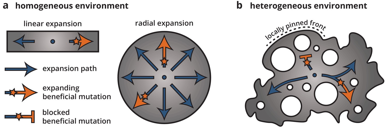
Cartoon of how environmental heterogeneity shapes evolutionary dynamics during range expansions.

In homogeneous environments (a), a locally established beneficial mutation (orange star), having survived genetic drift, can expand freely (arrows). By contrast, in heterogeneous environments (b), a beneficial mutation can become trapped in pinned stretches of the population, whereas expansion along open paths resembles a one-dimensional expansion.

https://doi.org/10.7554/eLife.44359.036

Figure 8

Download asset Open asset

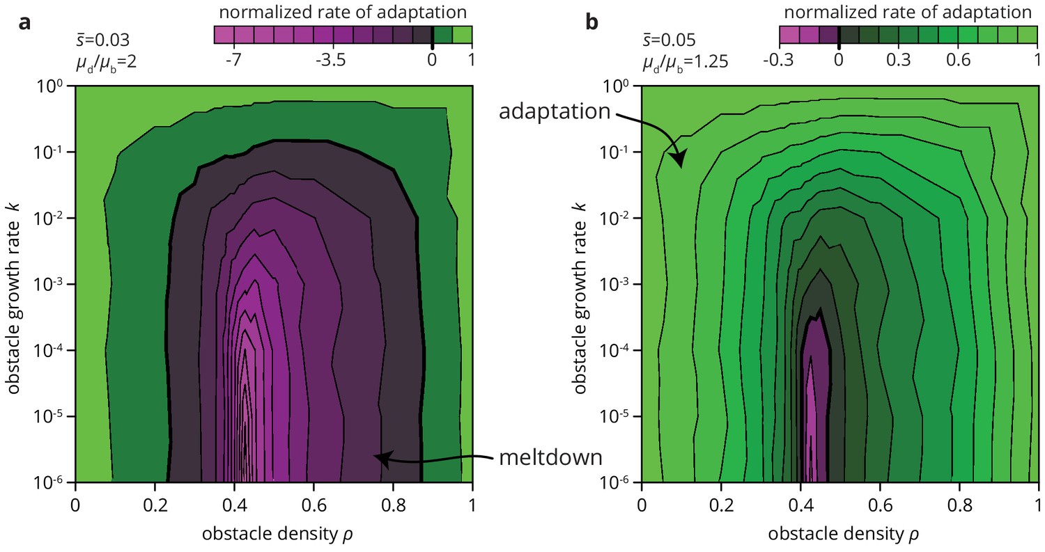
Environmental heterogeneity can alter evolutionary outcomes.

Rate of adaptation, defined as $\int D (s) s f_{MT} (s) 𝑑 s$ , computed for an exponential distribution of fitness effects $D (s)$ at various values of the environmental parameters $k$ and $ρ$ (see Materials and methods). The distribution of fitness effects is characterized by two parameters: the ratio $μ_{d} / μ_{b}$ of deleterious to beneficial mutation rate ( $μ_{d} / μ_{b} = 2$ in panel a, 1.25 in b), and $\bar{s}$ , the average fitness effect of a mutation ( $\bar{s} = 0.03$ in panel a, 0.05 in b). The rate of adaptation is normalized to its maximal value at $ρ = 0$ . Green tones correspond to adaptation (accumulation of beneficial mutations), magenta tones to accumulation of deleterious mutations.

https://doi.org/10.7554/eLife.44359.037

Tables

Table 1

Number of colonies assayed for each condition.

Pilot experiment one is reported in Figure 2—figure supplement 5, experiment two is reported in the main text.

https://doi.org/10.7554/eLife.44359.023

Experiment 1 (Figure 2—figure supplement 5)
dox (μg/ml)	0	0.2	0.4	0.6	0.8
n (smooth)	13	16	16	20	21
n (rough)	11	20	16	19	14
Experiment 2 (main text)
dox (μg/ml)	0	0.05	0.1	0.15	0.2	0.25	0.3	0.35	0.4	0.5	0.6	0.7	0.9	1.1
n (smooth)	8	30	37	26	31	27	32	41	30	36	30	24	31	28
n (rough)	20	24	32	20	32	25	19	22	31	28	18	19	27	29

Table 2

Characteristic exponents for the KPZ and QEW universality classes and measured in our simulations, which are in good agreement with the literature values in Amaral et al. (1995).

https://doi.org/10.7554/eLife.44359.038

Exponent	KPZ	This study ( $ρ = 0$ )	qEW	This study ( $ρ = ρ_{c}$ )
$α_{loc}$	1/2	0.5 ± 0.05	0.92 ± 0.04	0.9 ± 0.05
$α_{G}$	1/2	0.5 ± 0.05	1.23 ± 0.04	1.15 ± 0.05
$β$	1/3	0.3 ± 0.03	0.86 ± 0.03	0.78 ± 0.05
$θ$	N/A	N/A	0.24 ± 0.03	0.21 ± 0.03
$ζ$	2/3	0.66 ± 0.02	-	0.86 ± 0.04

Additional files

Transparent reporting form: https://doi.org/10.7554/eLife.44359.039
Download elife-44359-transrepform-v2.pdf

Download links

A two-part list of links to download the article, or parts of the article, in various formats.

Downloads (link to download the article as PDF)

Open citations (links to open the citations from this article in various online reference manager services)

Mendeley

Cite this article (links to download the citations from this article in formats compatible with various reference manager tools)

Matti Gralka
Oskar Hallatschek

(2019)

Environmental heterogeneity can tip the population genetics of range expansions

eLife 8:e44359.

https://doi.org/10.7554/eLife.44359

Share this article

Cite this article

Substrate roughness impacts bacterial colony morphology.

Likelihood of mutation rate for two different concentrations of doxycycline.

Figure 1—figure supplement 1—source data 1

Analysis of substrate roughness.

Figure 1—figure supplement 2—source data 1

Roughness of E.coli colonies on smooth and rough substrates, defined as the mean square deviation from the best-fit circle.

Figure 1—figure supplement 3—source data 1

Substrate roughness limits the efficacy of selection in bacterial colonies.

Figure 2—source data 1

Selective difference between mutants and wild type at different concentrations of doxycycline.

Figure 2—figure supplement 1—source data 1

Mutant frequency fMT as a function of radius r (see panel (c) for schematic), for smooth (a–b) and rough (d–e) colonies.

Figure 2—figure supplement 2—source data 1

Population size of colonies estimated by measuring colony height and area, and by resuspending and measuring the resulting optical density.

Figure 2—figure supplement 3—source data 1

Final frequency of mutants after 3 days of growth, on smooth (red) and rough (blue) plates.

Mutant frequency measured in colonies grown on smooth and rough substrates at five doxycycline concentrations (converted to fitness differences s as described in the main text) in a biological replicate experiment.

Figure 2—figure supplement 5—source data 1

Clone size distribution P(X>x) for colonies grown on smooth (a) and rough (b) substrates.

Figure 3—source data 1

A minimal model captures the change in colony morphology in heterogeneous environments.

Figure 4—source data 1

Characterization of Eden clusters with obstacles (k=0).

Figure 4—figure supplement 1—source data 1

A simple lattice model reproduces strong impact of environmental heterogeneity on evolutionary dynamics.

Figure 5—source data 1

Clone size distribution P(X>x) for colonies grown on smooth (a) and rough (b) substrates in simulations.

Figure 5—figure supplement 1—source data 1

Neutral lineage dynamics change with environmental heterogeneity.

Figure 6—source data 1

Environmental heterogeneity alters the shapes of mutant clones.

Figure 6—figure supplement 1—source data 1

Cartoon of how environmental heterogeneity shapes evolutionary dynamics during range expansions.

Environmental heterogeneity can alter evolutionary outcomes.

Number of colonies assayed for each condition.

Characteristic exponents for the KPZ and QEW universality classes and measured in our simulations, which are in good agreement with the literature values in Amaral et al. (1995).

Transparent reporting form

Downloads (link to download the article as PDF)

Open citations (links to open the citations from this article in various online reference manager services)

Cite this article (links to download the citations from this article in formats compatible with various reference manager tools)

Mutant frequency $f_{MT}$ as a function of radius $r$ (see panel (c) for schematic), for smooth (a–b) and rough (d–e) colonies.

Mutant frequency measured in colonies grown on smooth and rough substrates at five doxycycline concentrations (converted to fitness differences $s$ as described in the main text) in a biological replicate experiment.

Clone size distribution $P (X > x)$ for colonies grown on smooth (a) and rough (b) substrates.

Characterization of Eden clusters with obstacles ( $k = 0$ ).

Clone size distribution $P (X > x)$ for colonies grown on smooth (a) and rough (b) substrates in simulations.