State-dependent geometry of population activity in rat auditory cortex
- Champalimaud Center for the Unknown, Portugal
- University of Tübingen, Germany
- University of A Coruña, Spain
Figures
Figure 1
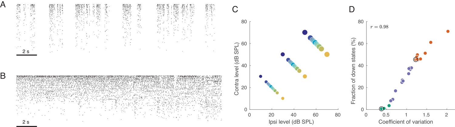
Population activity in rat auditory cortex during inactive and active states.
(A) Exemplary raster plot of 20 s of spontaneous activity in an inactive state ( neurons, sorted by firing rate). (B) Exemplary raster plot of 20 s of spontaneous activity in an active state ( neurons, sorted by firing rate). (C) Stimulus set. The auditory stimuli used throughout this study consisted of brief broad-band (5–20 KHz) noise bursts. The colors represent ILD and the dot sizes represent ABL. This color/size code is maintained throughout our study. (D) Relationship between coefficient of variation (CV) of the total spike count and the fraction of down states across all recorded sessions. Green/orange dots correspond to sessions that we will use as ‘active sessions’ and ‘inactive sessions’ (as the two extremes of the activation-inactivation continuum) but state-dependence will always be assessed using all recordings by regressing various quantities of interest against CV. Black circles show two sessions used for raster plots in (A), (B).
Figure 2 with 2 supplements
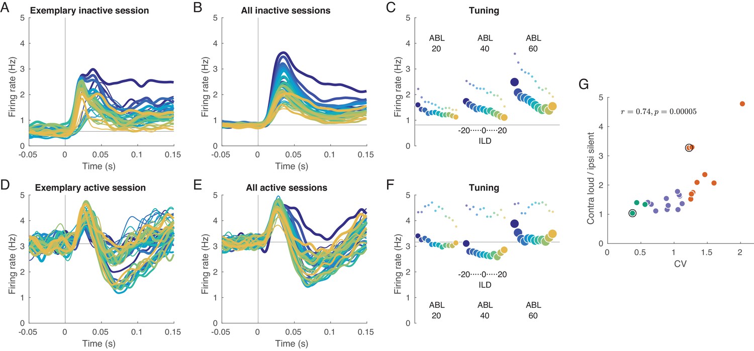
Evoked activity in inactive and active states, averaged across neurons.
(A) Exemplary inactive session. Each line is a population PSTH (peri-stimulus time histogram) corresponding to one stimulus (color coded as in Figure 1, line thickness corresponds to ABL). Population PSTHs were computed by averaging the Gaussian-smoothed ( ms) PSTHs of single neurons. (B) Mean of the population PSTHs across nine inactive sessions. (C) Average firing rate over 150 ms of stimulus duration for each stimulus, corresponding to panel B. Dots show the early response, defined as the average over 20–40 ms window. (D–F) The same for one exemplary and three overall active sessions. (G) The ratio of the evoked responses for the loudest, most contralateral stimuli and the most silent, most ipsilateral stimuli, computed for each session. Green dots are active sessions, orange dots are inactive sessions, black circles mark the two exemplary sessions used in (A) and (D).
Figure 2—figure supplement 1
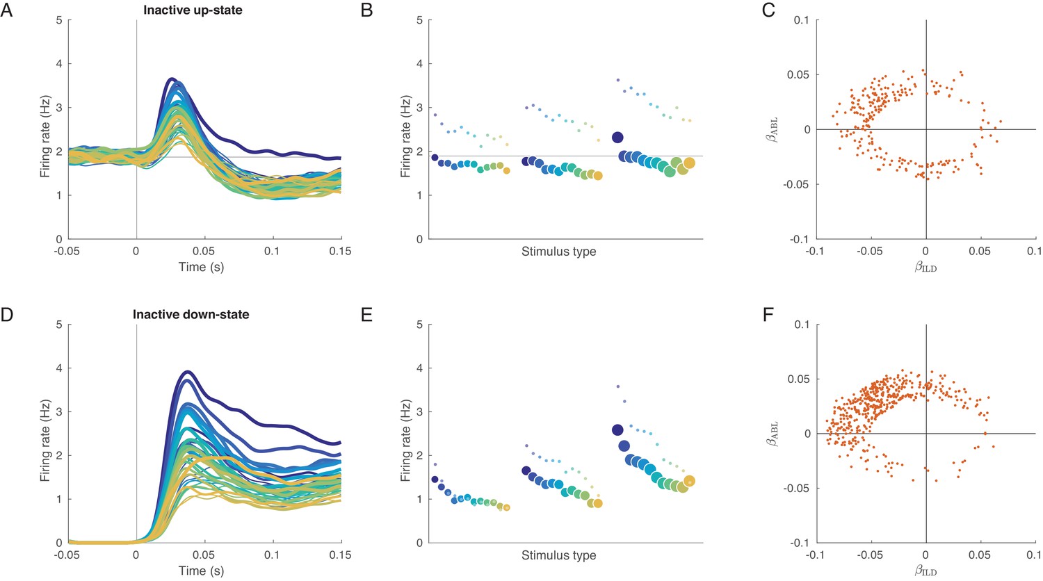
Evoked responses in the inactive sessions conditioned on the state before the stimulus presentation.
(A) Mean evoked response for each stimulus conditioned on the up-state (average over inactive sessions). Note some tuning in the early responses. (B) The tuning curve corresponding to (A), based on the 0–150 ms interval. Small dots: tuning curve based on the 20–40 ms interval. (C) Coefficients of linear fits to the up-state-conditioned tuning curves of all single neurons from all inactive sessions. Only neurons with significant linear tuning () are shown, as in Figure 3. Note that most significantly tuned neurons are located in the upper-left quadrant, corresponding to the loud contralateral preference. (D–F) The same for conditioning on the down-state. The loud contralateral preference is much more pronounced.
Figure 2—figure supplement 2
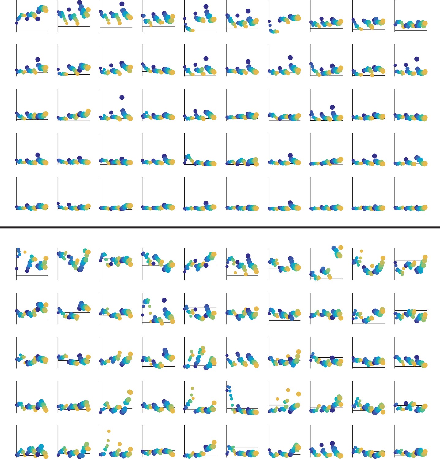
Tuning curves for 50 neurons with the highest average evoked responses in the exemplary inactive (top) and active (bottom) sessions.
Horizontal line shows baseline firing rate. Vertical line shows the scale from 0 to 20 Hz (same in all subplots).
Figure 3 with 5 supplements
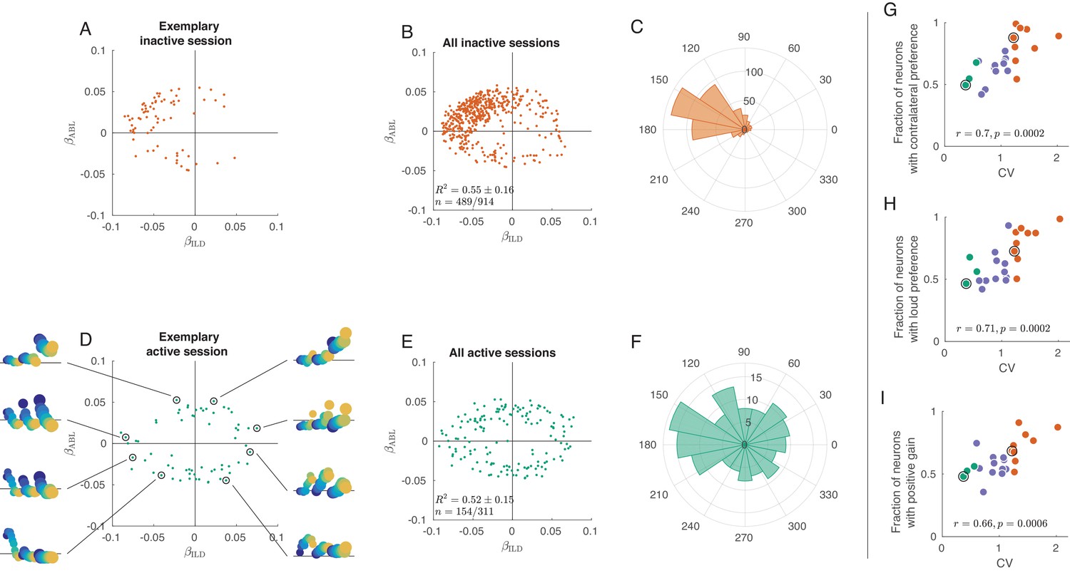
Tuning curves in inactive and active states.
(A) Single neurons from one exemplary inactive session. The tuning of each neuron was characterized with a linear additive model (see text); horizontal axis shows ILD coefficient and vertical axis shows ABL coefficient. Only neurons with significant tuning () are shown. (B) Single neurons ( neurons with significant tuning out of ) from nine inactive sessions. values correspond to the average ± standard deviation across the significantly tuned neurons. (C) Circular distribution of the neurons from panel (B). (D) Single neurons from one exemplary active session. Insets show tuning curves of eight exemplary neurons. (E) Single neurons ( neurons with significant tuning out of ) from three active sessions. (F) Circular distribution of the neurons from panel (E). (G) Fraction of neurons with contralateral preference (located to the left of the axis in panels (A) and (D)) across sessions. Green dots are active sessions, orange dots are inactive sessions, black circles mark the two exemplary sessions used in (A) and (D). (H) The same for the fraction of neurons with loud preference (located above the axis). (I) The same for the fraction of neurons with positive gain modulation (see text).
Figure 3—figure supplement 1
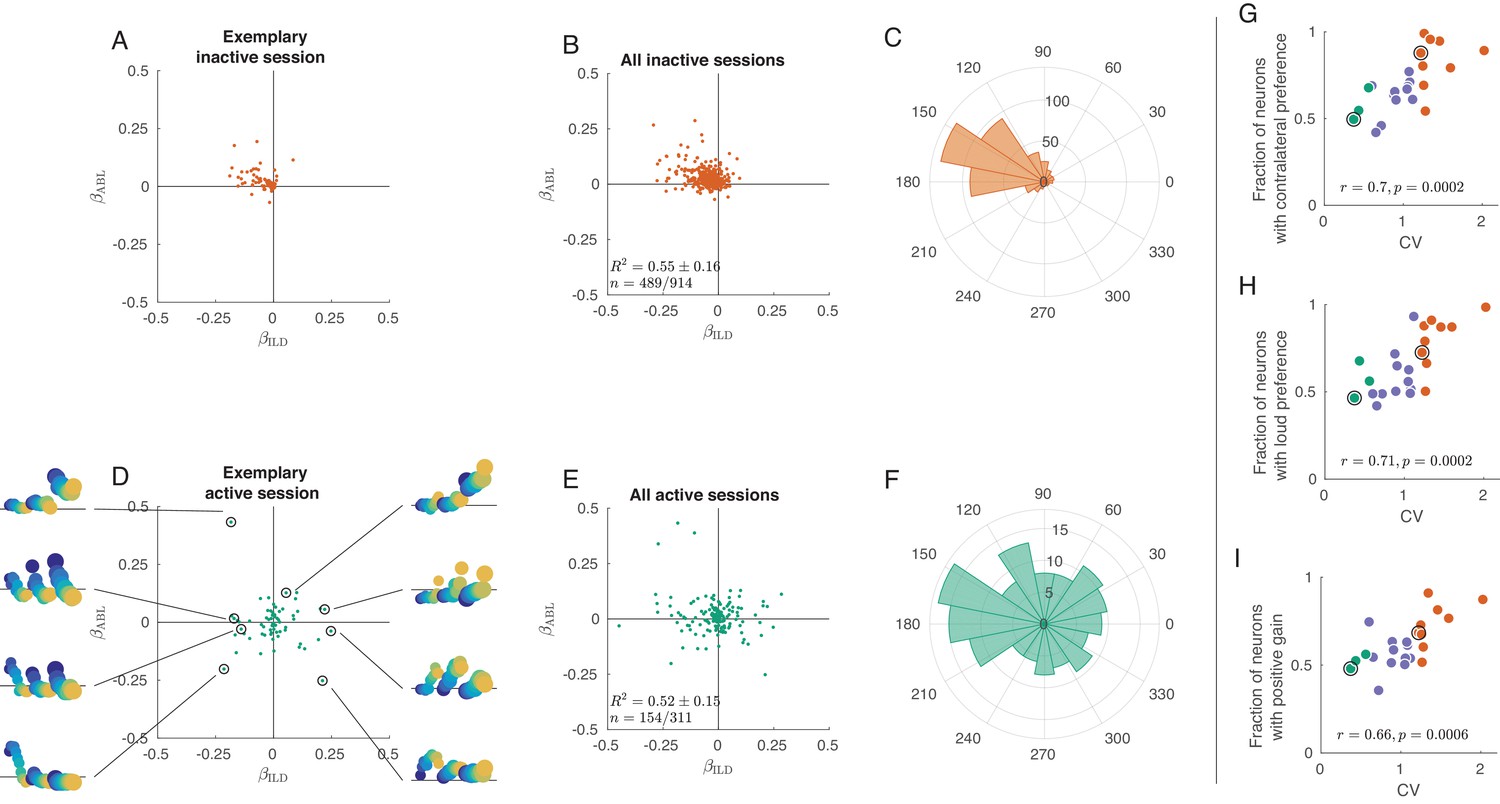
Exact analogue of Figure 3, but without z-scoring the tuning curves.
It only affects panels A, B, D, and E.
Figure 3—figure supplement 2
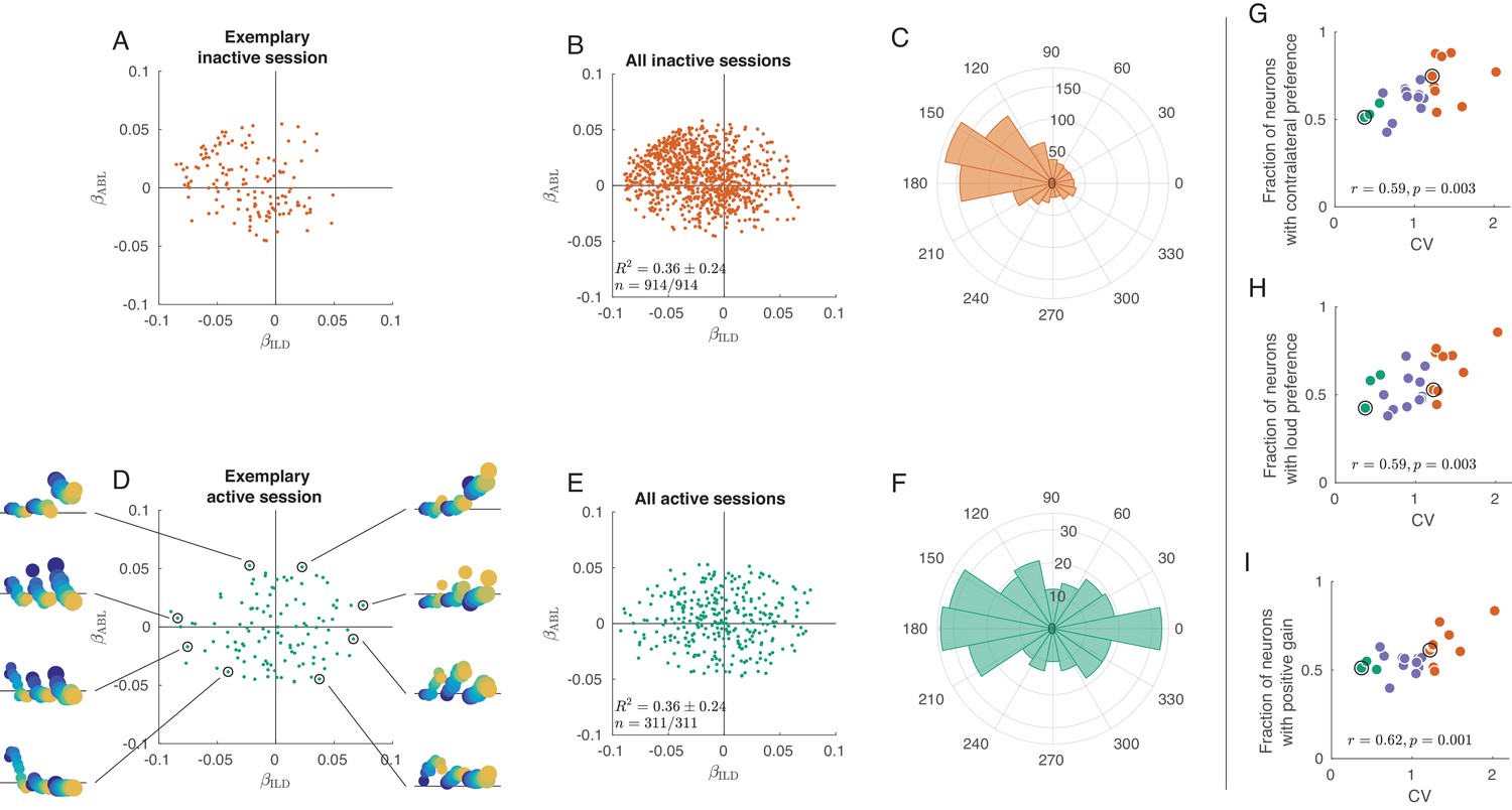
Exact analogue of Figure 3, but without filtering the neurons based on p-value.
https://doi.org/10.7554/eLife.44526.008
Figure 3—figure supplement 3
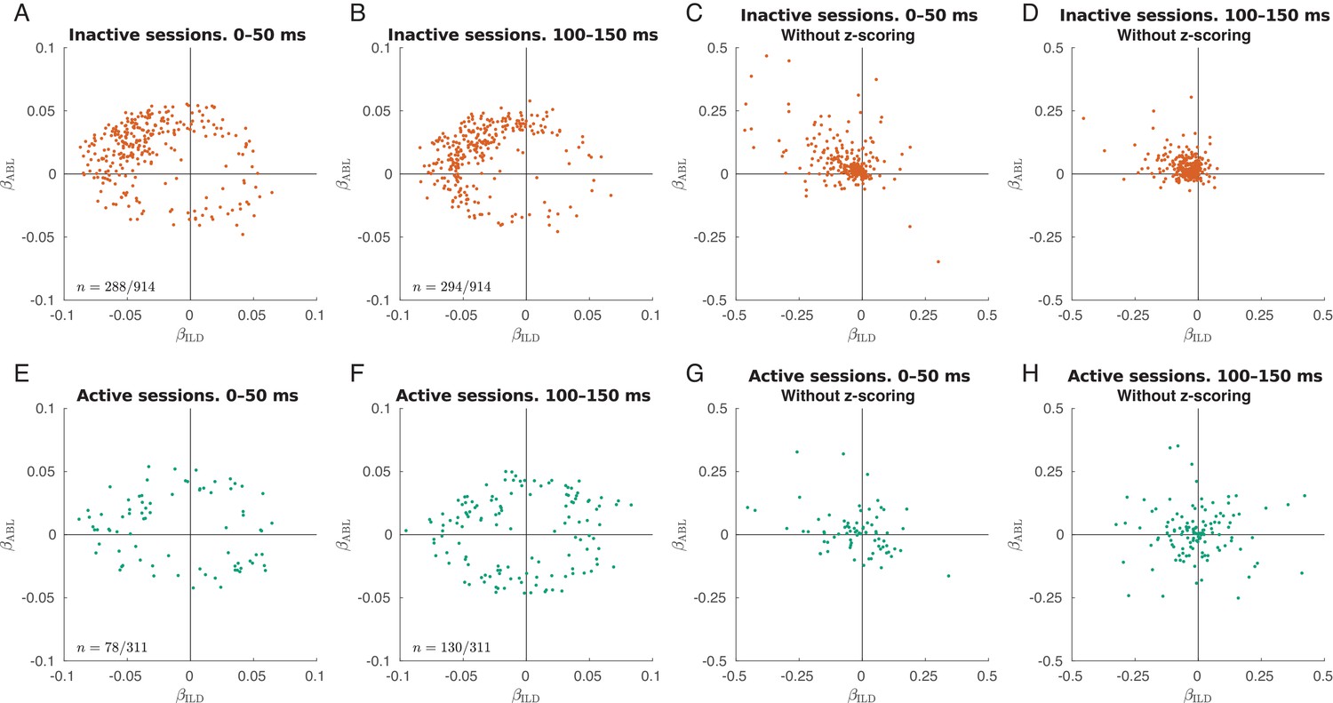
Early and late single neuron tuning.
Only neurons with significant linear tuning () are shown, as in Figure 3. (A) Distribution of the ILD coefficients and ABL coefficients across all neurons in the inactive sessions for evoked responses in 0–50 ms after stimulus onset. The early responses are mostly contralateral and loud preferring. The fraction of significantly tuned neurons is 31.5% (288/914). (B) The same but for evoked responses in 100–150 ms after stimulus onset. The fraction of significantly tuned neurons is 32.2% (294/914). (C–D) The same as in (A–B) but without -scoring the tuning curves. Here, one can see that the late responses are smaller than the early responses. (E–H) The same for all active sessions. In the last two panels, one can see that the high-firing early responses are mostly contralateral and loud preferring, while the late responses are more balanced. The fractions of significantly tuned neurons in the early and in the late responses were 23.1% (78/311) and 41.8% (130/311), a significant difference (, Fisher’s exact text). The distances between the ‘'early’' and the ‘late’' locations were very similar in both states: 0.036 ± 0.023 in the active state (mean ± SD for 117 neurons present in panels A and B) and 0.036 ± 0.023 in the inactive state (mean ± SD for 41 neurons present in panels E and F).
Figure 3—figure supplement 4
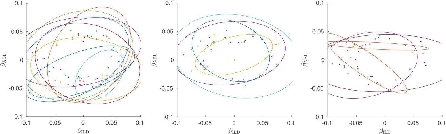
Single neurons from all three active sessions, colored by shanks.
Left subplot shows the same session as in Figure 3D), the other two subplots show two other active sessions. Ellipses show 90% coverage for each shank, assuming 2D Gaussian distributions. Only neurons with significant linear tuning () are shown, as in Figure 3.
Figure 3—figure supplement 5
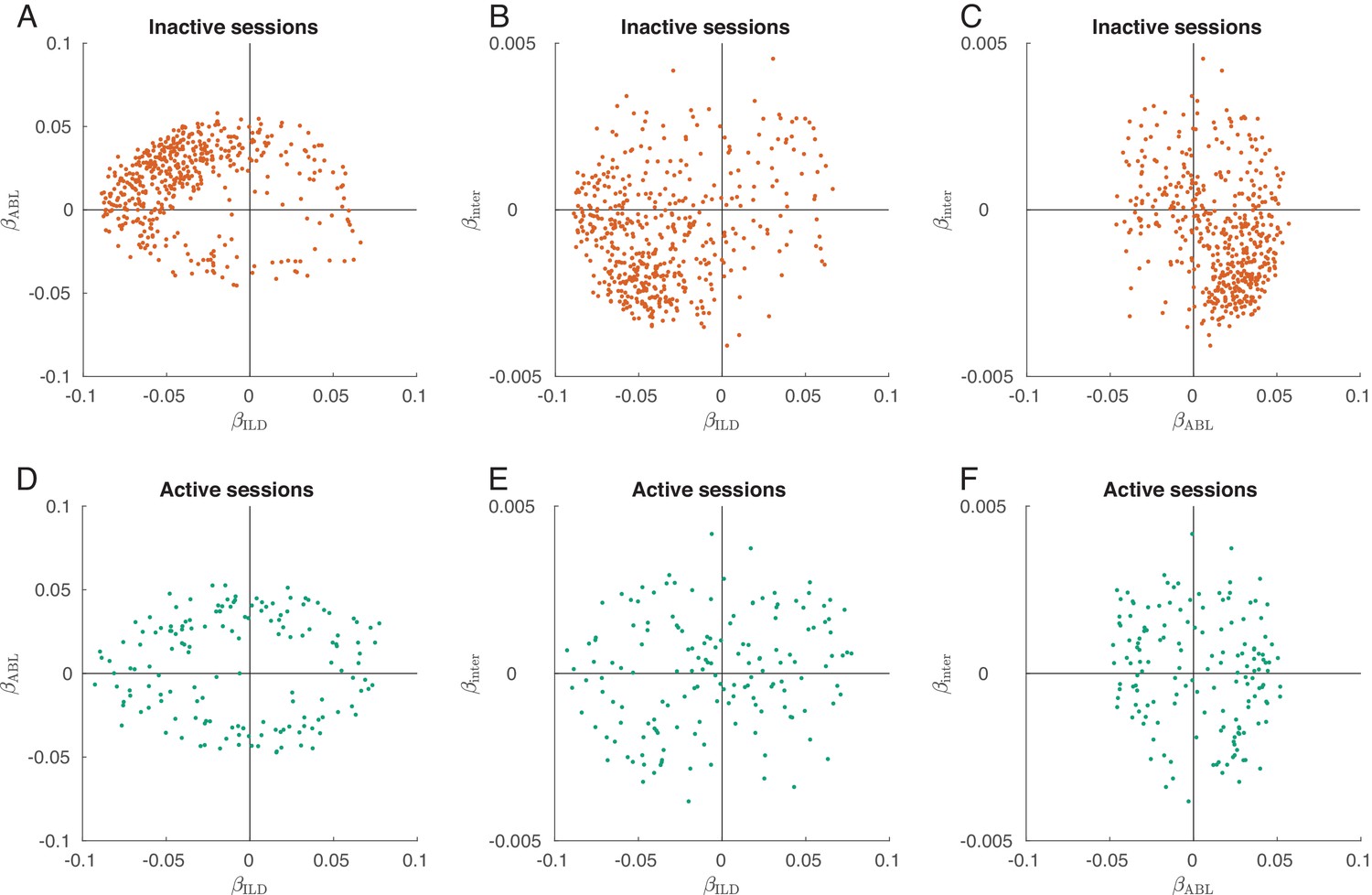
Interaction term in the linear model of single neuron tuning.
Only neurons with significant linear tuning () are shown, as in Figure 3. (A) Distribution of the ILD coefficients and ABL coefficients across all neurons in the inactive sessions. This panel reproduces Figure 3B. (B) Distribution of the ILD coefficients and coefficients across all neurons in the inactive sessions. Most neurons have negative ILD coefficient and negative interaction coefficient, meaning that increasing ABL increases the ILD tuning. This shows gain modulation. (C) Distribution of the ABL coefficients and coefficients across all neurons in the inactive sessions. (D–F) The same for the active sessions. Panel (D) reproduces Figure 3D. If large ABLs increased the slope of ILD tuning (that in active sessions is sometimes positive and sometimes negative) then we would expect to see a positive correlation on panel (E). Correlation is indeed positive () but rather weak.
Figure 4
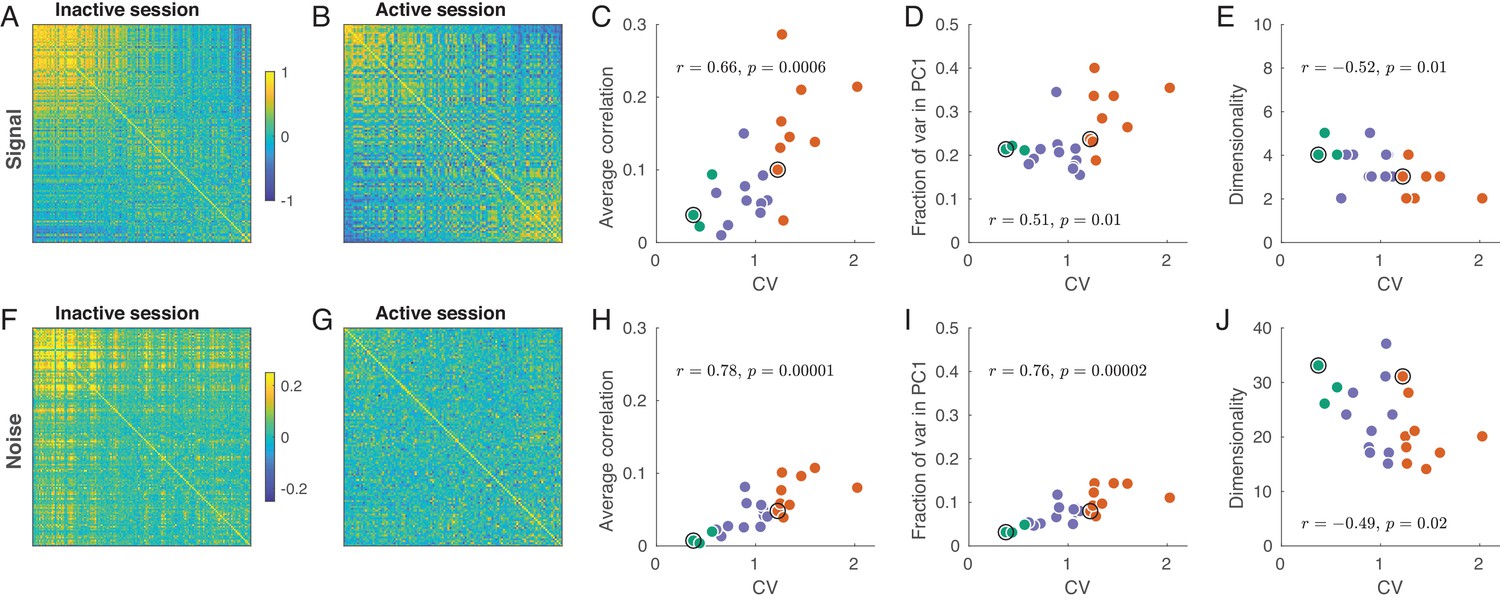
Signal and noise correlations in inactive and active states.
(A) Signal correlation matrix in an exemplary inactive session. Neurons are ordered by their ILD tuning from contralateral (top/left) to ipsilateral (bottom/right). (B) Signal correlation matrix in an exemplary active session. Neurons are ordered in the same way. (C) Average off-diagonal signal correlation as a function of CV. Here and in the other panels green dots are active sessions, red dots are inactive sessions, black circles mark the two exemplary sessions. (D) Fraction of variance explained by the first principal component of the signal correlation matrix as a function of CV. (E) Estimated dimensionality of the signal correlation matrix as a function of CV. (F–J) The same for noise correlation matrices. Note that the color scale in (F), (G) is different from (A), (B).
Figure 5 with 1 supplement
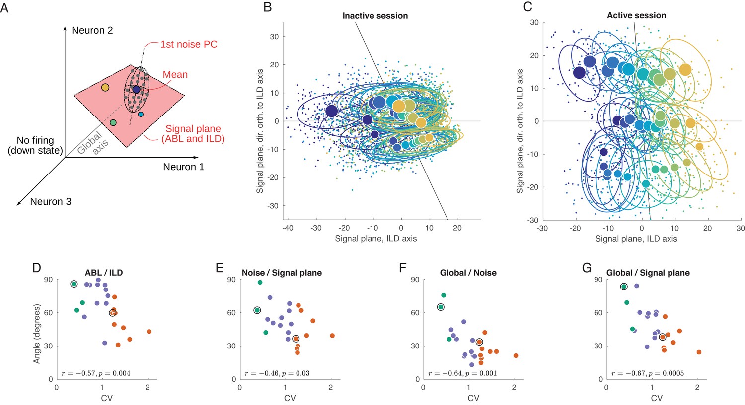
Geometry of population activity in inactive and active states.
(A) Schematic of the population geometry analysis. The firing rate of each neuron forms a dimension, and evoked activity in each trial is represented by a dot in this space. (B) Projection of all single trials on the signal plane in one exemplary inactive session. Big dots and ellipses show averages and 50% coverage ellipses for each stimulus. Color coding as in previous figures. Horizontal black line is the ILD axis, the other black line is the ABL axis. (C) The same for one exemplary active session. (D–G) Relationship between CV and the angles between the ILD axis and the ABL axis (D), between the noise axis and the signal plane (E), between the noise axis and the global axis (F), and between the global axis and the signal plane (G).
Figure 5—figure supplement 1
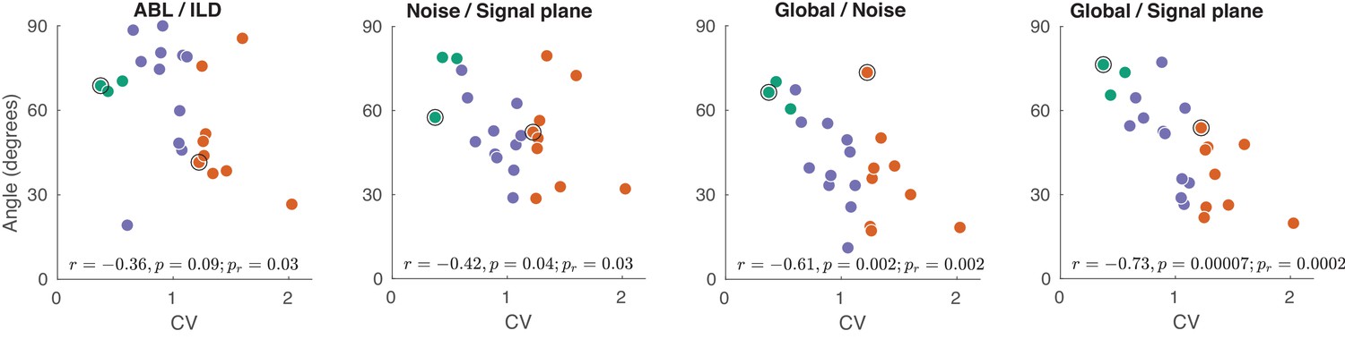
The exact analogue of Figure 5D–G, but using spike counts in the 0–50 ms window, instead of 0–150 ms.
All correlations (and p-values) apart from ABL/ILD stay very similar to the ones in Figure 5D–G. The correlation of ABL/ILD angle with CV drops to −0.36 with . It seems that the decrease might be mostly explained by one strong outlier (the session with the smallest angle). For that reason we added a p-value for the slope of robust regression (robustfit in MATLAB) to all panels (). For the ABL/ILD angle it was .
Figure 6 with 2 supplements
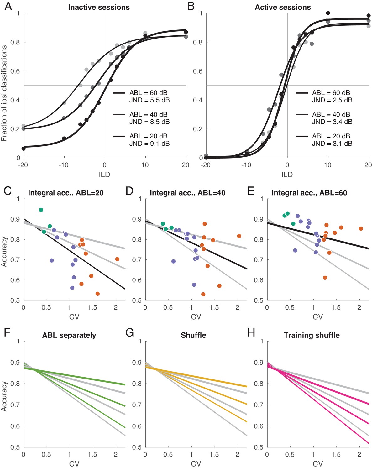
Decoding analysis in inactive and active sessions.
(A) Population neurometric curves in inactive sessions. Dots show the fraction of ipsilateral classifications when classifying the sign of ILD (from grey to black, ABL = 20 dB to ABL = 60 dB), averaged across inactive sections. Curves show logistic fits. (B) Population neurometric curves in active sessions. (C–E) Integral classification accuracy for across sessions for each ABL separately. Gray lines show constrained linear fits for each ABL. Black lines highlight the fit corresponding to the respective scatter plot. (F) The change of linear fits when one uses separate decoder for each ABL (green). (G) The change of linear fits after shuffling trials for each neuron in each condition (yellow). (H) The change of linear fits after shuffling the training sets only (magenta).
Figure 6—figure supplement 1
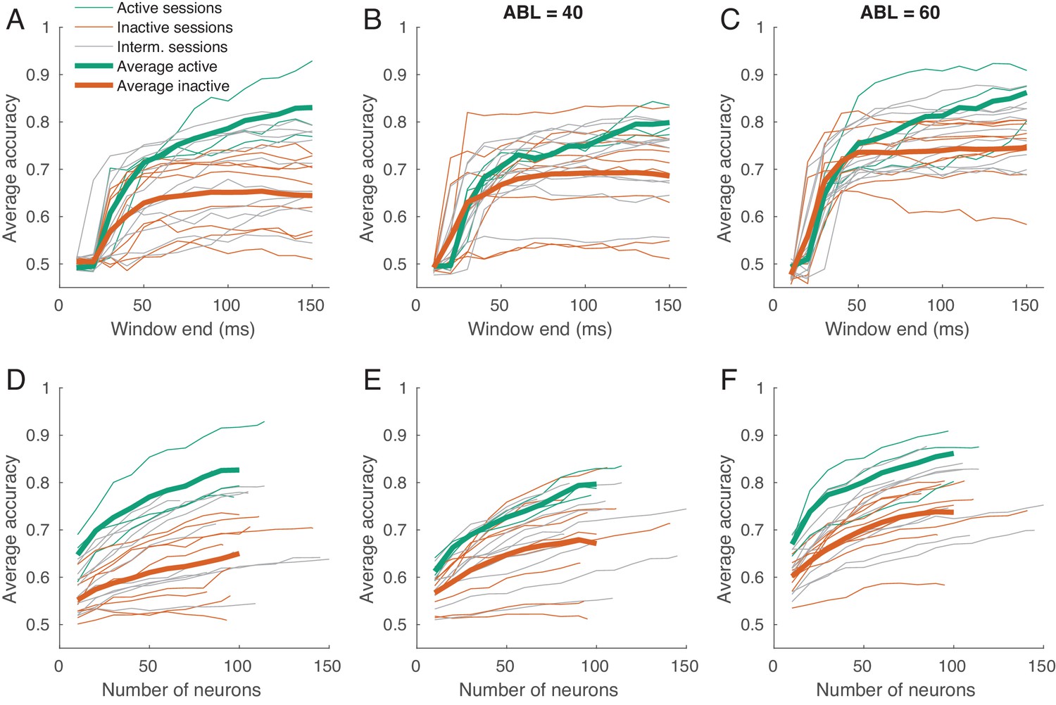
Classification accuracy as a function of spike count window length and of the number of neurons.
(A–C) Time-resolved average classification accuracy (average over all ILD values) for each ABL separately, using the spike counts in time window ms. The window end changed between 10 and 150 ms in steps of 10 ms. Thin lines are individual sessions, thick lines are averages over active and inactive sessions. (D–F) The average classification accuracy (average over all ILD values) for each ABL separately using a subsampled pool of neurons (averages over 10 random subsamples are shown). The number of neurons ranged between 10 and the number of neurons in a session, in steps of 10. Thin lines are individual sessions, thick lines show averages across sessions. The averages over sessions are shown until 100 neurons only.
Figure 6—figure supplement 2
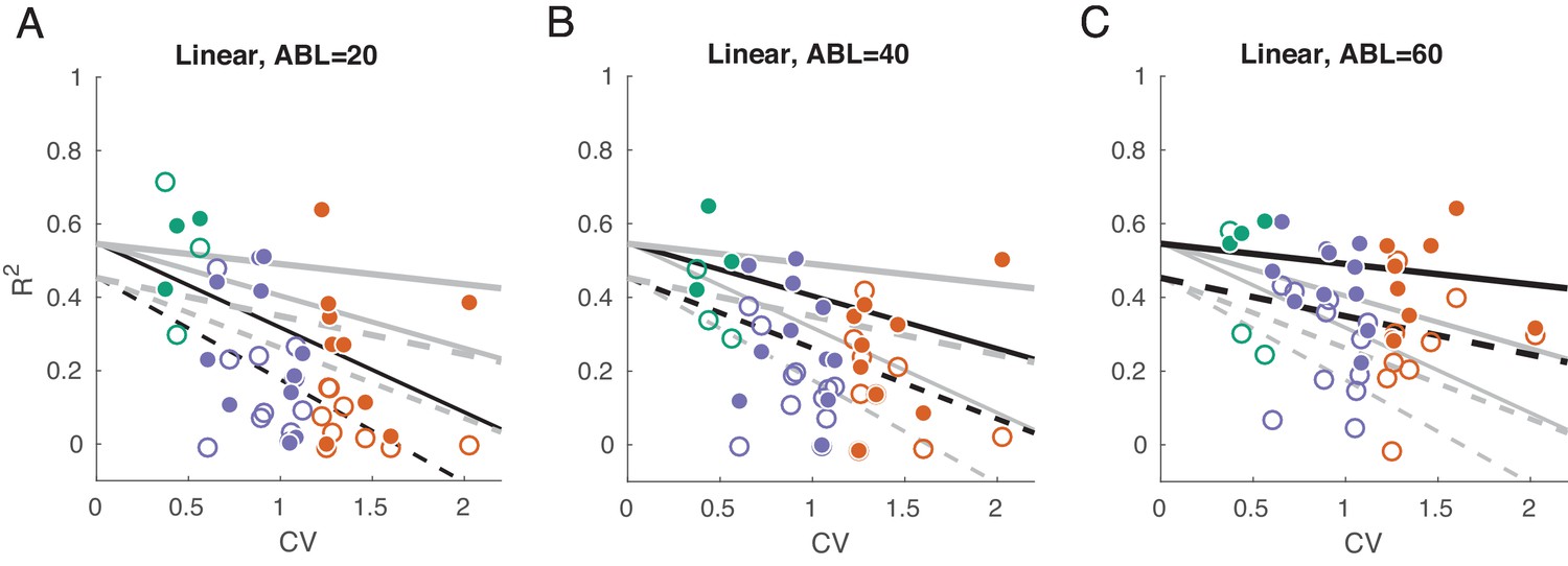
We used linear decoding of ILD, separately for the contralateral and ipsilateral sounds and separately for each ABL.
Linear fits are the form . This fits a linear dependency between CV and the goodness of ILD prediction (cross-validated ), and we allow the slope and the intercept to change with ABL and be different for ipsilateral () and contralateral () decoding. This model has only six coefficients instead of 12 that six independent regressions would have but this simpler model was preferred by both AIC and BIC . (A–C) of linear decoder of ILD value, separately for each ABL and for ipsilateral and contralateral ILD values. Grey lines show constrained linear fits (solid lines: contralateral decoding, dashed lines: ipsilateral decoding). Black lines highlight fits corresponding to the respective subplot. Solid dots show values for contralateral decoding, open circles show values for ipsilateral decoding.
Videos
Video 1
Three-dimensional subspace spanned by the signal plane and the global axis in the exemplary inactive and in the exemplary active sessions.
https://doi.org/10.7554/eLife.44526.015Additional files
-
Transparent reporting form
- https://doi.org/10.7554/eLife.44526.019
Download links
A two-part list of links to download the article, or parts of the article, in various formats.
Downloads (link to download the article as PDF)
Open citations (links to open the citations from this article in various online reference manager services)
Cite this article (links to download the citations from this article in formats compatible with various reference manager tools)
State-dependent geometry of population activity in rat auditory cortex
eLife 8:e44526.
https://doi.org/10.7554/eLife.44526


