Functional and anatomical specificity in a higher olfactory centre
- MRC Laboratory of Molecular Biology, United Kingdom
- University College London, United Kingdom
- The Francis Crick Institute, United Kingdom
- Howard Hughes Medical Institute, United States
- University of Cambridge, United Kingdom
Figures
Figure 1 with 1 supplement
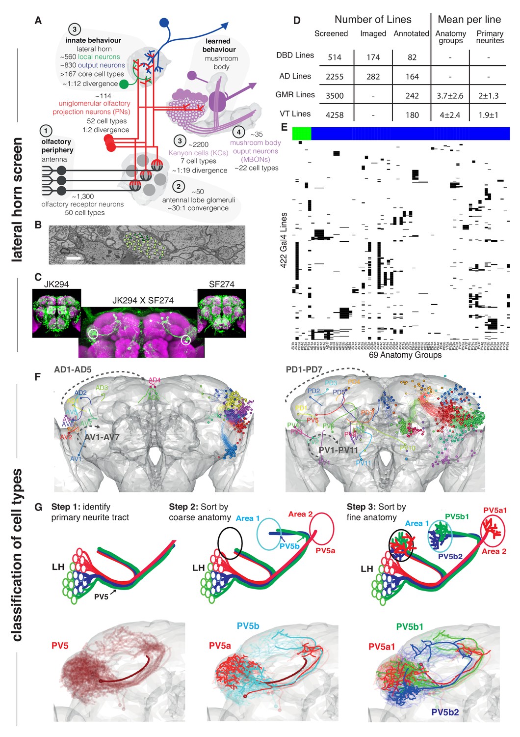
Screen for genetic driver lines labeling Lateral Horn Neurons.
(A) Flow diagram following olfactory information to third order neurons of the LH and MB calyx. (B) Section through the PV5 primary neurite tract within the EM data; each profile was identified as an LHN (circles) or non LHN (triangles) by tracing to the first branch point. Scale bar 1 μm. (C) Sample Split-GAL4 intersection with parental lines inset. Cell body locations marked with white circle. (D) Summary table for the genetic screen. (E) Matrix summarizing which driver lines contained which anatomy groups (colored LHON = blue, LHLN = green). The vast majority of genetic driver lines labeled only a few LH anatomy groups. NB these data are also available as a supplementary spreadsheet. (F) Anterior (left) and posterior (right) views of the different LHN primary neurite tracts demonstrating the broad origin of LHNs. Grey dashed arrow indicates the order of increasing tract numbers for ventral PNTs (Lower arrow) and dorsal PNTs (above). The entry point into the brain rather than soma location was the point of reference for naming tracts. (G) Upper panels, cartoons summarizing the logic of the LHN naming system, lower panels, the PV5 primary neurite as an example. Note this includes only 3 out of 24 cell types in PV5. For each cell type one cell is highlighted (thick lines).
Figure 1—figure supplement 1
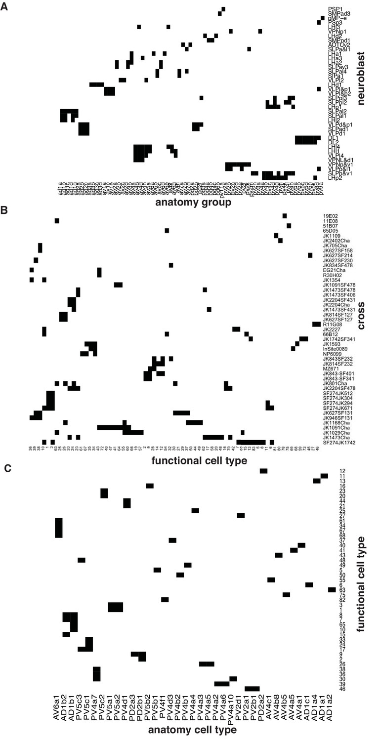
Summary of anatomical and functional screen.
(A) Matrix showing putative neuroblast origin for anatomy groups identified in the screen. (B) Matrix showing physiology classes together with the cross from which they were recorded. (C) Matrix connecting each of the physiology classes with the anatomy cell types to which it belongs.
Figure 2 with 2 supplements
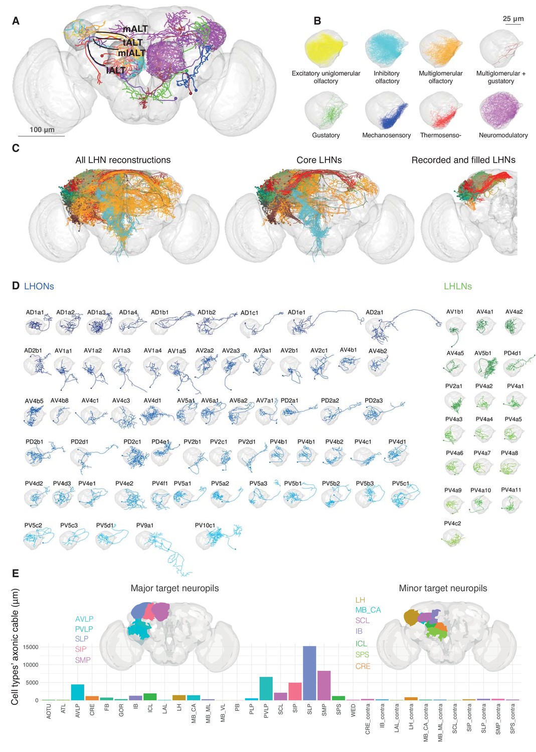
Single cell anatomy of the Lateral Horn.
(A) Sample single projection neurons with axonal projections in the LH, showing all major axon tracts and sensory modalities that provide input. (B) Close up of the LH with axonal arbors for all FlyCircuit neurons of each presumptive sensory modality. (C) Overview of our annotated LHN skeleton library showing all skeletons with LH arbors, core LHN cell types (see Figure 2—figure supplement 1) and those neurons reconstructed after electrophysiological recording in the present study. Neurons colored by anatomy group. (D) Visualization of single exemplars for all cell types for which we have >=3 skeletons in the library, or from which we made electrophysiological recordings in this study. Output neurons in blue, local neurons in green. (E) Bar chart showing, for each target neuropil, the total axonal cable length contributed by all core LHONs (calculated as sum of mean for each identified cell type). Brains plots show in major (> 3 mm axonal cable) and minor (1–3 mm) targets of LHONs. Brain neuropil according to Ito et al. (2014); mALT, medial antennal lobe tract, tALT, transverse antennal lobe tract, mlALT, medio-lateral antennal lobe tract, lALT, lateral antennal lobe tract.
Figure 2—figure supplement 1
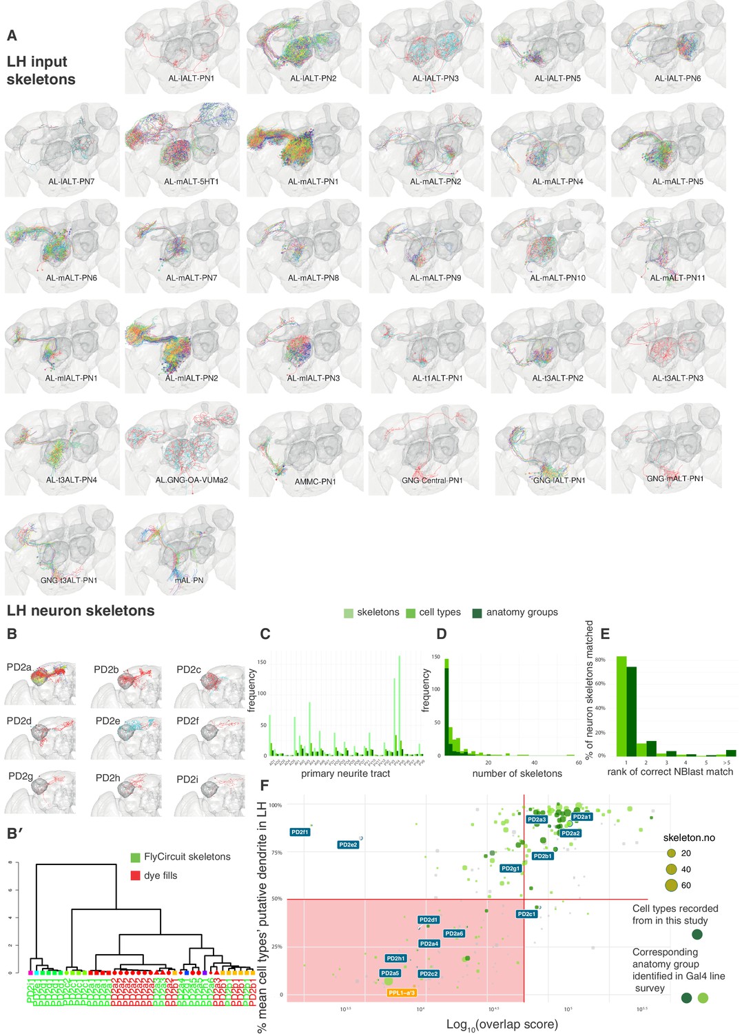
Summary of neuron skeleton data for LHNs and PNs.
(A) FlyCircuit PN skeletons co-registered in a standard brain and separated by anatomy group (panels). Each skeleton is plotted in a different color. The number of skeletons is determined by frequency in the FlyCircuit dataset not the number of cells in a single brain. LH, MB lobes and AL shown in darker grey. (B) Example LHN primary neurite cluster, PD2, broken down into its constituent anatomy groups (panels) and cell types (colors). (B’) Using NBLAST to disambiguate cell types and anatomy groups. Dendrogram based on hierarchical clustering of NBLAST scores. Node shape and color indicate different anatomy groups. Leaf color indicates whether each skeleton is from the FlyCircuit dataset or a dye-fill from this study. (C) The number of skeletons, cell types and anatomy groups in the LHN dataset in each primary neurite cluster. (D) Histogram showing the number of skeletons for each LHN anatomy group and cell type. (E) Using NBLAST to match a neuron skeleton to the correct anatomy group. Each skeleton in the dataset was removed, NBLASTed against the rest, mean scores were taken per anatomy group, and anatomy groups ranked. Bar chart shows percentage of skeletons matched to, 1, the correct anatomy group and, >=2, incorrect anatomy groups. (F) Defining a ‘core' set of LHNs. Scatter plot shows cell type plotted against the Log10 of their overlap score (see Materials and methods) with PN termini and the proportion of their dendritic arbor (see Materials and methods) in the standard LH (Ito et al., 2014). Horizontal decision boundary at 50%, vertical decision boundary at 50000, red box, non ‘core' LHNs. The dopaminergic MB input neuron, PPL1-a'3 (Aso et al., 2014a), is flagged in orange as an example of a non-core LHON. Points bounded in blue indicate cell types shown in panel A. Points in chartreuse and dark green (rather than gray) indicate cell types belonging to anatomy groups identified in the Gal4 lines we screened. We made electrophysiological recordings from cell types in dark green.
Figure 2—figure supplement 2
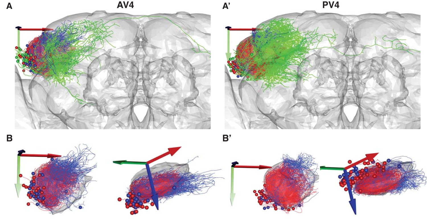
Local vs. Output AV4 and PV4 clusters.
(A) A frontal view of the two largest tracts containing local interneurons. Local anatomy group AV4a (A) and PV4a (A’) are colored red. Similar clusters with local arborization just outside the LH AV4b (A) and PV4b (A’) are colored blue. The rest of the anatomy groups in these primary neurite tracts are colored green. (B) Same as A but showing frontal (left) and dorsolateral (right) views with the two main anatomy groups only.
Figure 3 with 1 supplement
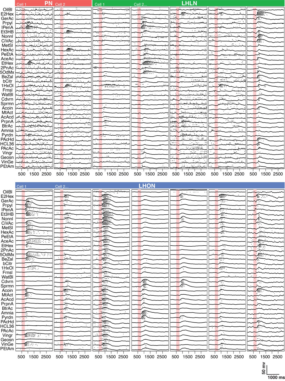
Comparing odor responses of second and third order olfactory neurons.
Raster plots for two PNs (red), five LHLNs (green), and seven LHONs (blue). Each odor was presented 4 times to each cell with a 250 ms valve opening starting 500 ms after recording (red bar). For each odor the voltage response of the four trials was averaged (continuous line) while rasters show the spiking response for each presentation. Note the progressive reduction in baseline firing rate and sparseness between PNs and LHLNs, and LHONs. Odors abbreviated on the left can be identified from a supplementary spreadsheet.
Figure 3—figure supplement 1
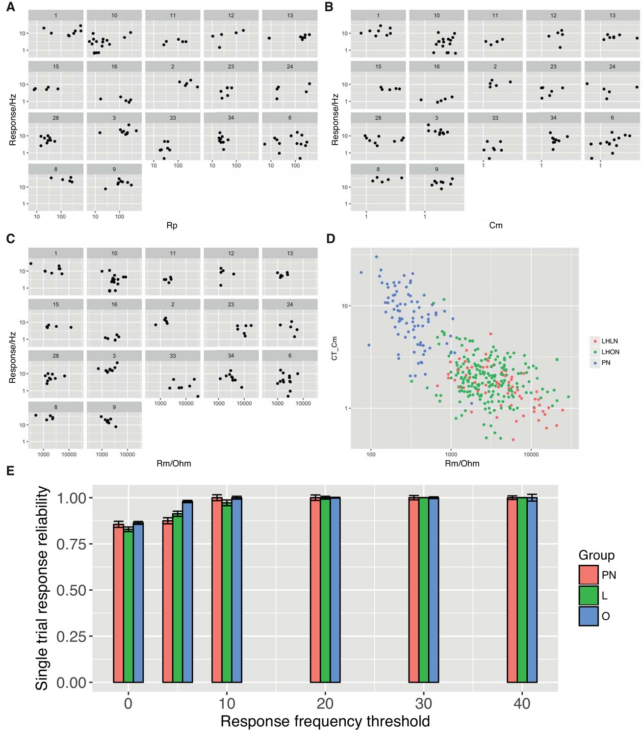
Cell Physiolgical Parameters.
For each physiology class the mean response is plotted against the access resistance (A), the cell capacitance (B), and the membrane resistance (C). (D) Cell capacitance is plotted against membrane resistance with cells colored according to their group (PN, LHLN, LHON). (E) Single trial response reliability using different mean response thresholds.
Figure 4
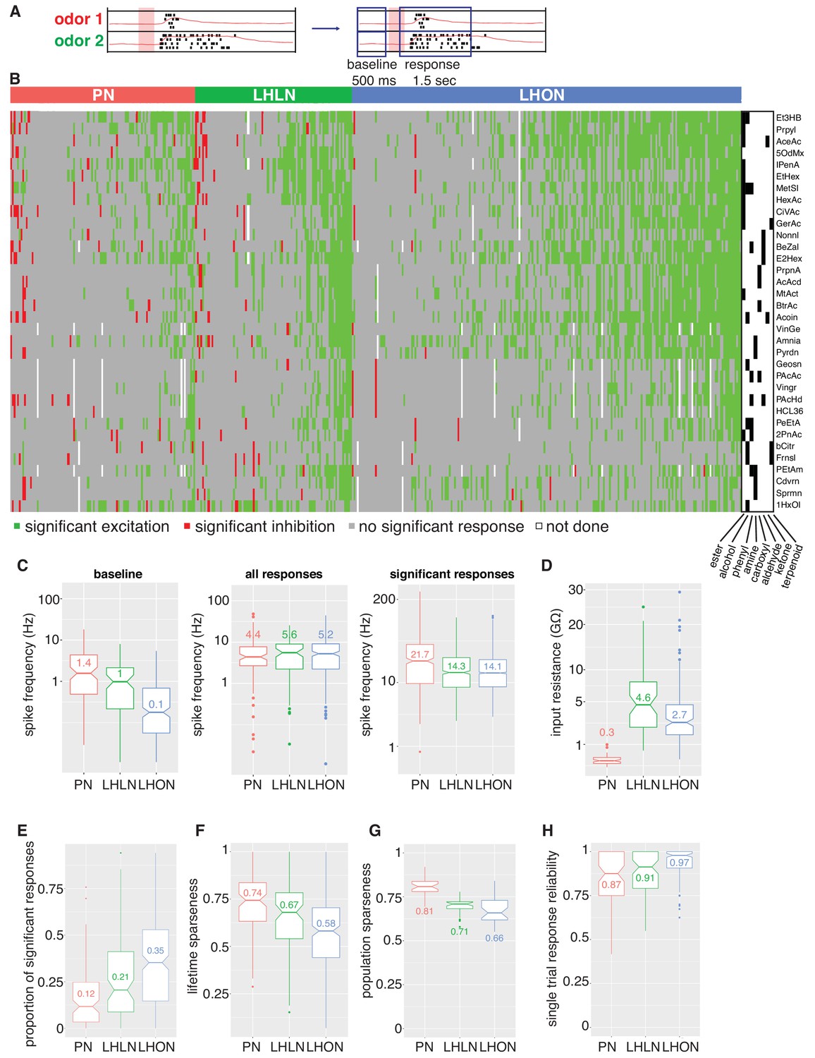
Population summaries of second and third order olfactory neurons.
(A) Diagram of time windows used when identifying significant spiking responses (see Materials and methods). (B) Matrix showing significant spiking responses of PNs, LHLNs, and LHONs (colors match Figure 3) to different odors. A black and white matrix shows the chemical groups of the different odors (see supplementary spreadsheet). (C) Comparing firing rates of PNs, LHLNs, and LHONs. Baseline firing rate (baseline), firing rate in the response window (all responses), and firing rate in the response window for significant responses only (significant responses). LHONs have a lower baseline firing rate and, when using significant response only, a lower odor-evoked firing rate then PNs. (D) Input resistance of PNs, LHLNs, and LHONs. (E) Different measures of sparseness of odor responses in PNs, LHLNs, and LHONs showing that LHONs are broader then PNs. (F) Single trial response reliability using a threshold of 5 Hz for PNs, LHLNs, and LHONs. Responses were reliable for all three groups with LHON responses slightly more reliable probably due to differences in baseline firing rate.
Figure 5
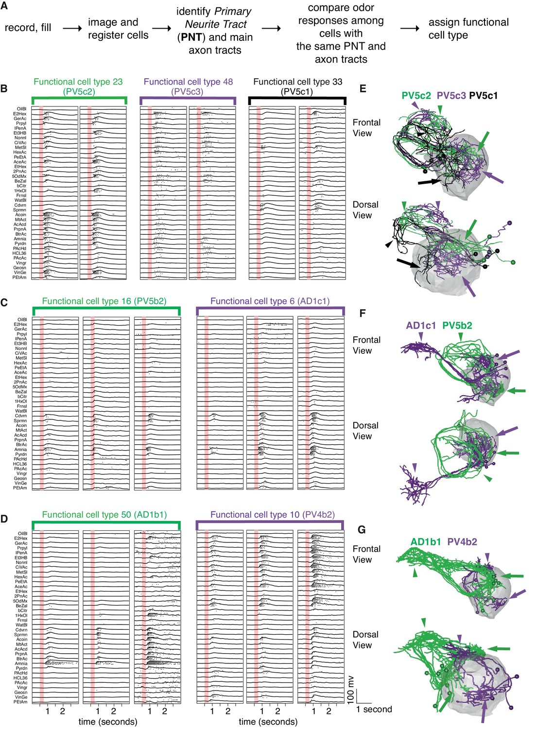
Comparing physiology and anatomy of different cell types.
(A) Our pipeline for identifying cell types. (B) Odor responses for three cell types (n = 2 neurons each) belonging to the same anatomy group. Each pair of neurons that belongs to the same functional cell type are marked by a colored bar with the functional cell type number. Although the three cell types have really similar anatomy, their responses are clearly very different. (C) Example of two functional cell types (n = 3 neurons each) that have very similar response properties but very different anatomy. (D) Some cell types showed significant variability in the strength of their odor responses across recorded cells while still showing consistency (n = 3 neurons for each of 2 cell types). (E, F, G) Frontal (top) and dorsal (bottom) images of dye filled neurons correspond to the functional cell types in B-D. Colored arrows (dendritic) and arrowheads (axonal) pointing to the arbors of each cell type. Altogether the figure demonstrates cons functional cell type classification.
Figure 6
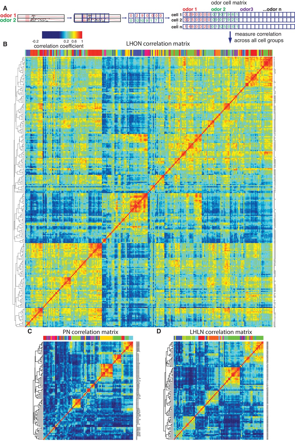
Cross-correlation clustering of odor response data for PNs, LHLNs, and LHONs.
(A) Analysis pipeline for generating the cell-odor response correlation matrix and measuring correlation across cells. Responses were binned (blue squares, 50 ms) and the mean firing rate was calculated for each time bin. For each cell, the responses to all odor, ware concatenated into a single vector and a matrix of all the cell odor responses was generated. This cell-odor matrix was used to calculate the Pearson’s correlation between the odor responses for all pairs of cells. (B–D) Heatmaps of the resultant cross-correlation matrices for LHONs, PNs and LHLNs, respectively. To allow comparison all three heatmaps share the same color scale for the correlation coefficient (top left) demonstrating a higher correlation between LHONs as well as considerable higher level of off-diagonal correlation structure.
Figure 7 with 1 supplement
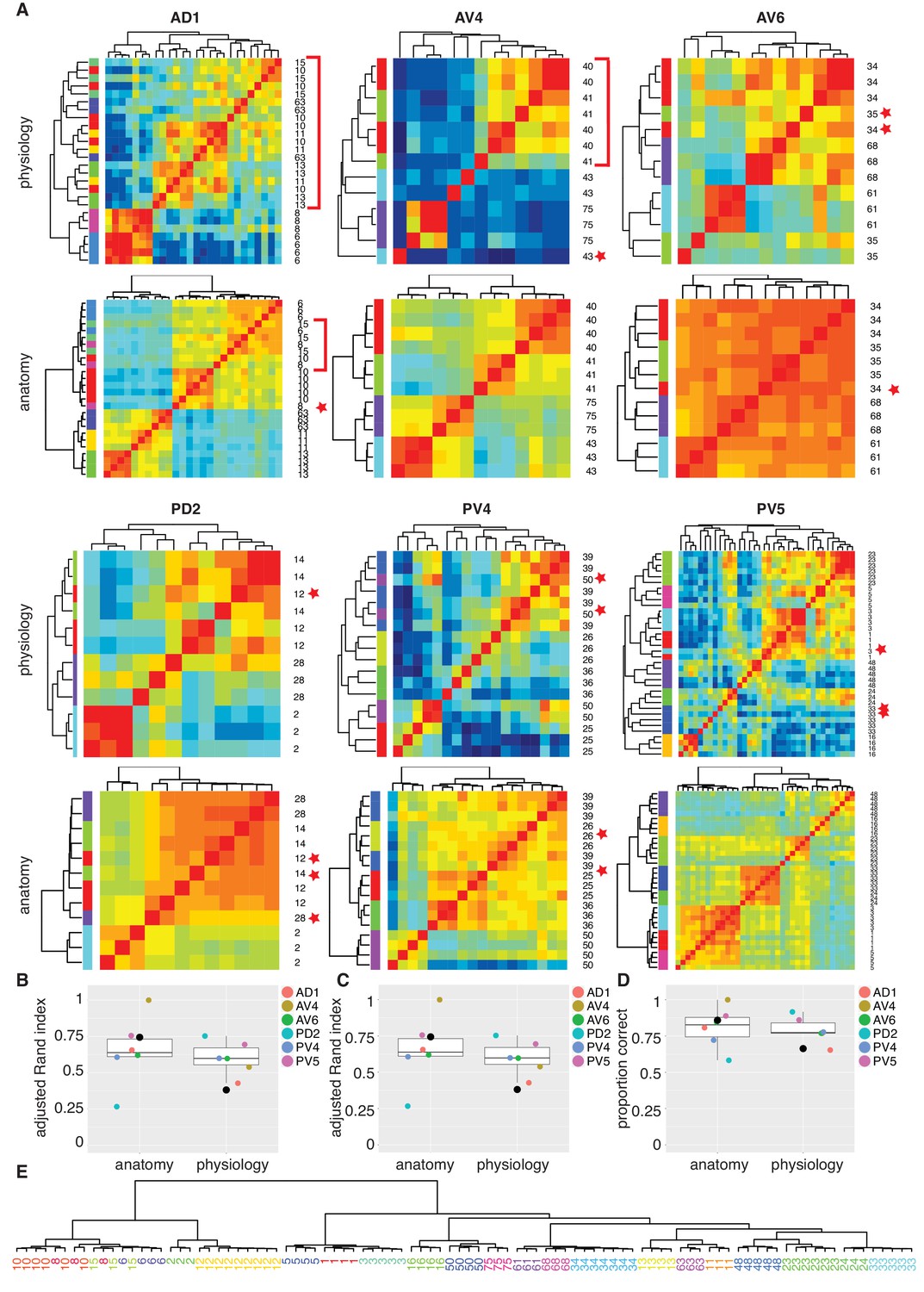
Comparing anatomy and physiology classification.
(A) Cross correlation matrix of odor responses and fine anatomy (NBLAST) for the same cells. Cells were divided according to their PNT. Only classes with at least three traced cells were used. We highlighted areas of misclassification with either a star (single mis-classified cell) or a red bar for a section of several cells. Correlation matrices for six primary neurites were organized in pairs with physiology on top and Anatomy below. Color scale for all physiology Correlation matrices and all anatomy Correlation matrices is the same. (B) Summary comparing Adjusted Rand Index clustering score for each primary neurite tract by physiology and anatomy. Black dot in B to D marks the results of analyzing the entire data set together. (C) Summary comparing Adjusted Rand Index clustering score for each primary neurite tract by physiology and anatomy after correcting class labels in two cases. (D) Summary comparing percent correct clustering score for each primary neurite tract by physiology and anatomy after class correction. (E) NBLAST clustering of all functional cell types with >=3 traced cells after merging two cases of indistinct cell types (see Figure 7—figure supplement 1 for details). Note the excellent agreement between the anatomical clustering and our manually defined functional cell types.
Figure 7—figure supplement 1
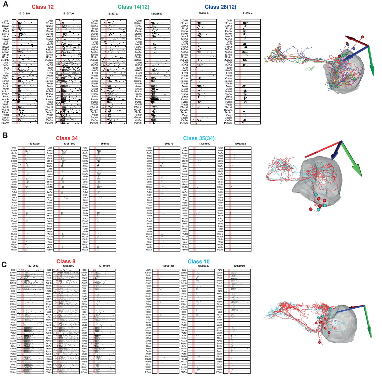
Morphologically and Physiologically Similar Classes.
We examined three cases in which both odor tuning and anatomy had significant similarities. (A) Functional cell types 12, 14, and 28 are very similar in their anatomy and their odor responses were showed high variability. We therefore decided to merge them into a single class (12). (B) We had initially separated cell types 34 and 35 due to a large difference in response strength, however in the absence of a difference in anatomy and given that they responded to the same odors we decided to merge them into a new class (34). (C) Classes 8 and 10 are similar both in physiology and anatomy but nevertheless significant differences still enabled them to be separated.
Figure 8
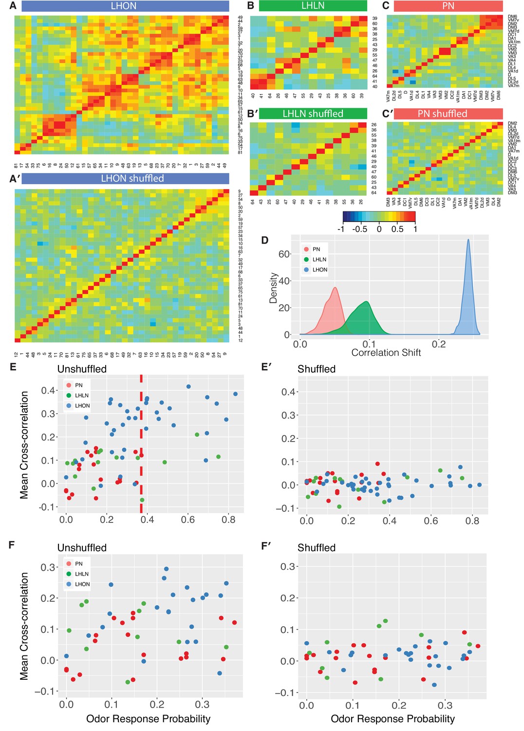
Comparing odor coding of LHNs with their inputs.
(A–C) Aggregated correlation heatmaps for LHONs, LHLNs, and PNs generated by calculating a mean odor response profile for each cell type and then computing the correlation matrix across all cell types. (A’–C’) Aggregated correlation heatmaps calculated after shuffling odor labels. For comparison all six heatmaps share the same color scale. (D) Histogram of mean correlation shift by randomizing the odor labels (n = 1000 replicates). (E, E’) For each cell type the mean cross-correlation against all other cell types was plotted against the proportion of significant odor responses of that cell type, either with or without shuffling of odor labels. (F, F’) As for E but only including correlation between sparse cell types (left to the red line in E indicating p(response)¡0.36, the highest odor response probability for PNs). Note that F and F’ are not just a subset of E and E’ as we recalculated the mean cross-correlation after selecting the sparsest LHON and LHLN cell types. Altogether the figure shows that the higher cross-correlation in LHON responses is due to LHONs sampling of odor space less homogeneously than PNs and not because of increased tuning breadth of LHONs or the increased number of LHON classes.
Figure 9
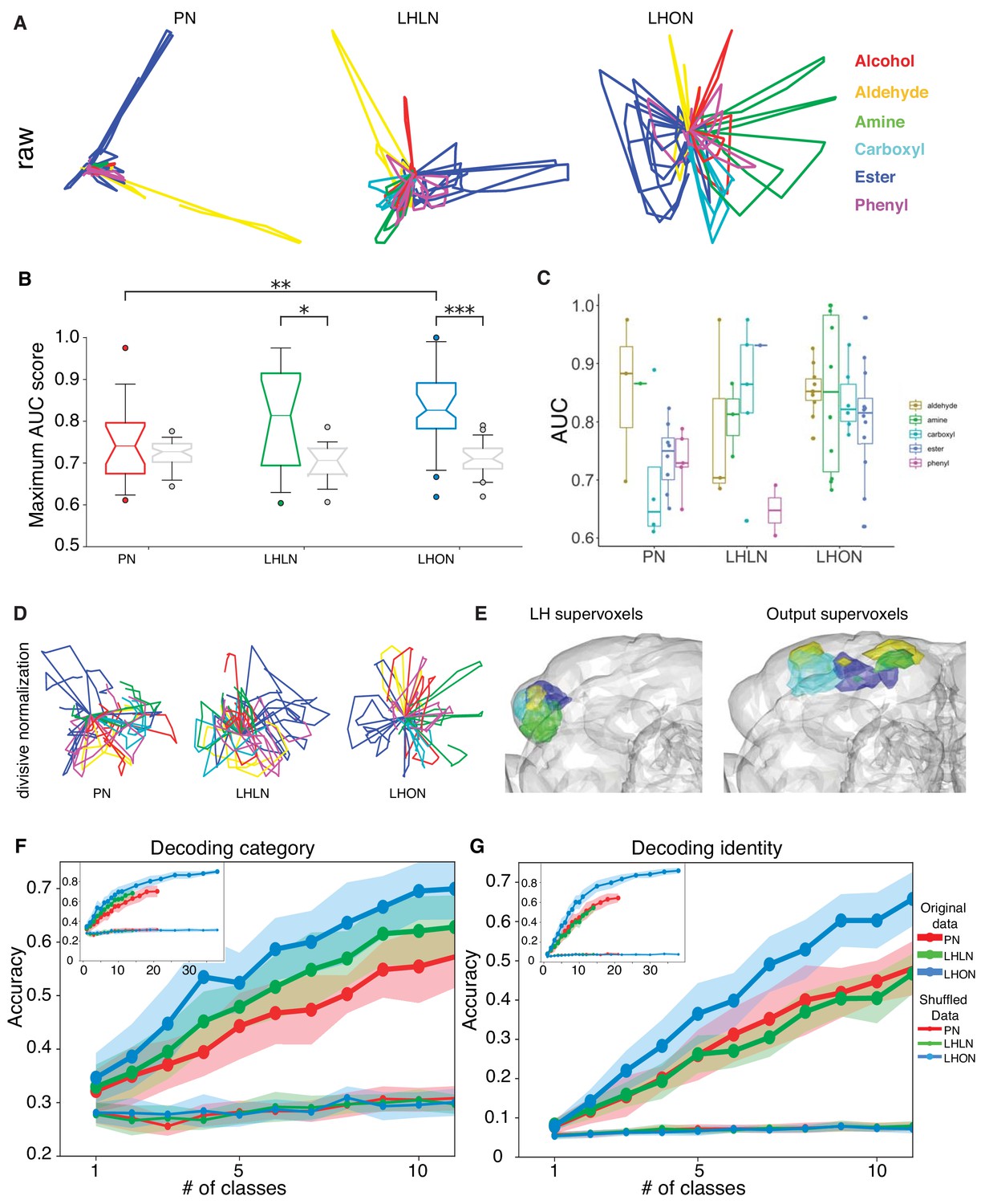
Odor categorization in the LH.
(A) Population representations of odors. Responses are projected into the spaces of the second and third principal components, and color-coded by odor category. (B) Distribution of AUC scores for PNs and LHLNs, and LHONs. An AUC score of 0.5 indicates no information about odor category. Box = 25–75% centiles, line = median, whiskers 5–95% centiles, notch indicates bootstrap 95% confidence interval of the median. LHON odor responses convey more category information than PNs (), one-sided Mann-Whitney U-test (C) Distribution of AUC scores for each population divided into the different odor categories (D) PCA analysis after divisive normalization. (E) Mapping of the different odor categories to brain voxels (see Materials and methods: Odor coding analysis). (F–G) Decoding accuracy of linear support vector classifiers (SVC) trained to perform category (F) or identity (G) classification using different numbers of cell classes. The main figure shows the result of using 1 to 10 classes while the inset shows the result of using all available classes for each group. Altogether we show that LHONs are better at encoding odor chemical categories than PNs.
Figure 10

Structural connectivity between antennal lobe glomeruli and third order olfactory neurons.
(A) Input tuning curves for a set of EM reconstructions comprising 17 LHLNs, and 29 LHONs (Schlegel, Bates et al. ms in prep) whose dendrites are restricted to the LH. The x axis is rank ordered by the number of synaptic inputs from uniglomerular PNs from each of 51 glomeruli. (B) Dot plots showing distribution of number of input glomeruli for LHLNs, and LHONs, and the number of dendritic claws for KCs. KC claw number data was based on light microscopy (LM) data presented in Caron et al. (2013) or EM reconstructions in Zheng et al. (2018). Some LHNs receive no excitatory uniglomerular PN input; their feed-forward input may come from multiglomerular or non-olfactory projections to the LH. Group means are shown by large black dots, error bars indicate a single standard deviation from the mean. See also Materials and methods. In sum, a reasonable cut-off for the observed structural connectivity in our EM-reconstructed wiring diagram reveals that the average LHN and each KC may sample the same number of glomeruli, via uniglomerular excitatory olfactory PNs. LHNs exhibit a larger standard deviation; some LHNs may act in a specific labelled line for unique and behaviorally significant odors, others may need to sample a larger number of ethologically connected odors more broadly.
Tables
Table 1
LHN tracts characterized in electron microscopy data.
match the Primary Neurite Tract nomenclature defined in Figure 1. indicates whether the tract contains output or local neurons or a mix of both. indicates the total number of profiles within the tract. indicates the sampling based estimate for the number of LHNs in the tract. gives a 90% confidence interval.
| Tract | Type | Profiles | Est. LHNs | Range | Recorded |
|---|---|---|---|---|---|
| AV4 | LHLN>>LHON | 324 | 252 | 244–259 | Yes |
| PV4 | LHLN>LHON | 158 | 155 | 152–158 | Yes |
| PV2 | LHLN>>LHON | 193 | 92 | 81–102 | Yes |
| PD3 | LHLN | 75 | 59 | 43–75 | |
| PD4 | LHLN | 88 | 22 | 10–33 | |
| –LHLNs– | 838 | 578 | 555–602 | ||
| AV3 | LHON>LHLN | 144 | 140 | 140 | |
| PD2 | LHON | 193 | 128 | 128 | Yes |
| PV5 | LHON | 127 | 119 | 119 | Yes |
| AD1 | LHON | 286 | 116 | 102–130 | Yes |
| AV6 | LHON | 323 | 106 | 96–115 | Yes |
| AV2 | LHON>>LHLN | 98 | 63 | 49–77 | Yes |
| AD3 | LHON | 59 | 59 | 59 | |
| AV7 | LHON | 141 | 48 | 25–70 | |
| AV1 | LHON | 33 | 25 | 25 | |
| AV5 | LHON | 108 | 17 | 7–27 | |
| PV3 | LHON | 52 | 12 | 0–25 | |
| AD2 | LHON | 52 | 0 | 0 | |
| –LHONs– | 1616 | 832 | 797–868 | ||
| –Total– | 2454 | 1411 | 1368–1454 |
Additional files
-
Supplementary file 1
Summary odor response data for recorded neurons expressed as baseline subtracted spike rate (Hz).
- https://doi.org/10.7554/eLife.44590.018
-
Supplementary file 2
The drive lines used in this study to target specific populations of neurons.
More specific driver have now been reported our sister paper, Dolan et al. (2019).
- https://doi.org/10.7554/eLife.44590.019
-
Supplementary file 3
A zip file containing SWC format neuronal skeletons.
- https://doi.org/10.7554/eLife.44590.020
-
Supplementary file 4
The metadata associated with each skeleton, including cell type annotations.
- https://doi.org/10.7554/eLife.44590.021
-
Supplementary file 5
The odors set used in our study, including details of their chemical categories and their CAS numbers.
- https://doi.org/10.7554/eLife.44590.022
-
Supplementary file 6
Summary of the EM connectivity between the EM reconstructed PNs and LHNs in Figure 10.
- https://doi.org/10.7554/eLife.44590.023
Download links
A two-part list of links to download the article, or parts of the article, in various formats.
Downloads (link to download the article as PDF)
Open citations (links to open the citations from this article in various online reference manager services)
Cite this article (links to download the citations from this article in formats compatible with various reference manager tools)
Functional and anatomical specificity in a higher olfactory centre
eLife 8:e44590.
https://doi.org/10.7554/eLife.44590


