Imaging single-cell blood flow in the smallest to largest vessels in the living retina
- University of Rochester, United States
Figures
Figure 1 with 1 supplement
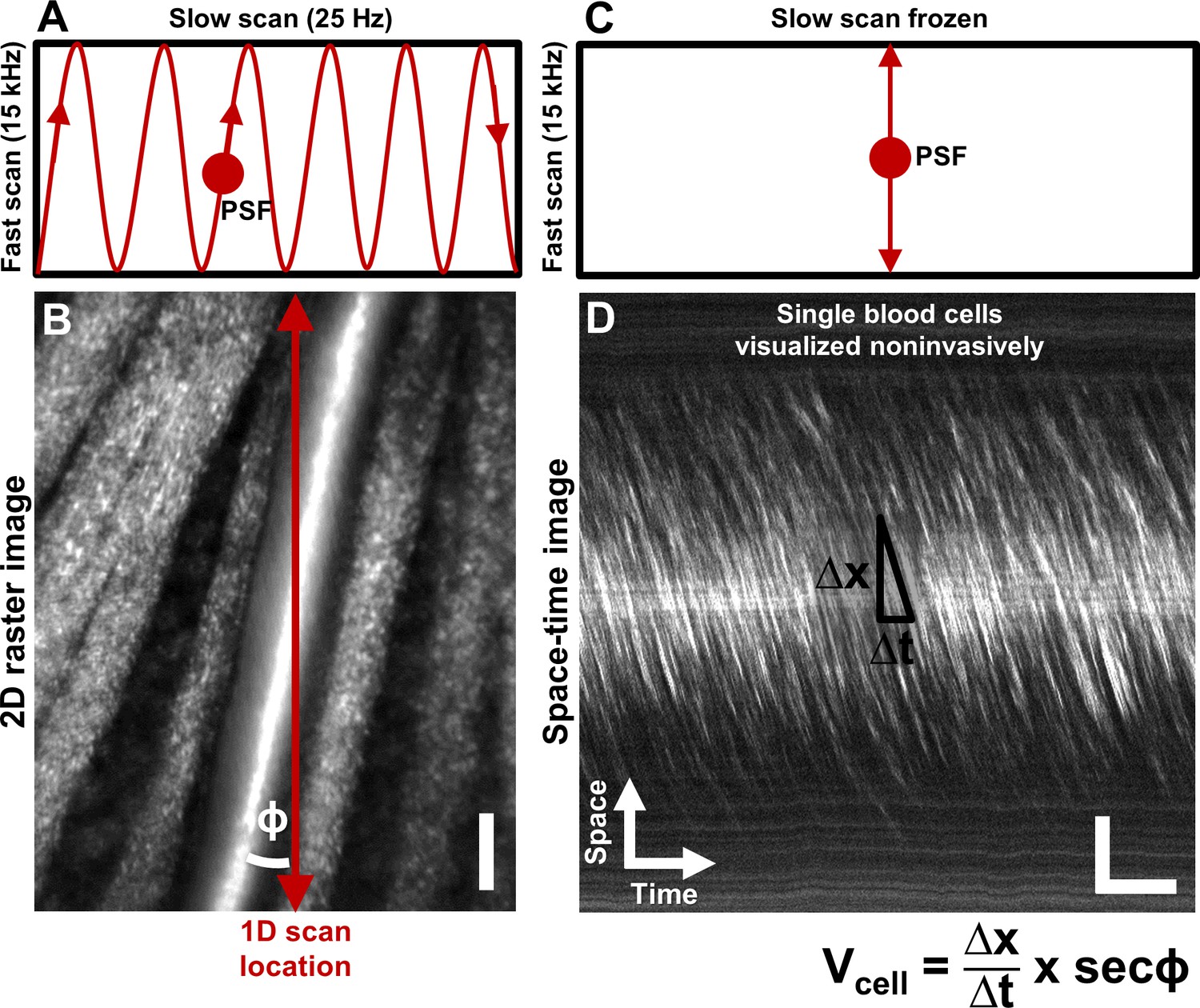
Noninvasive imaging of single blood cells and their velocity.
(A) 2D scan pattern of an adaptive optics scanning light ophthalmoscope (AOSLO) that produces a conventional Cartesian or XY image, shown in B. Two orthogonal scanners raster scan the point spread function (PSF) to produce a video (frame rate = 25 Hz, defined by the slow scan rate). (B) A Cartesian image of a first generation arteriole emerging from the optic disk, imaged with 796∆17 nm direct backscatter. The arteriole (intersected by red arrow) is surrounded by nerve fiber bundles. Typically, 250 frames (10 s) of such a video are recorded (Video 1) and averaged to produce the image shown. The scanning field of view was 4.80° x 3.73°. For visualization only, image brightness has been increased by 20–40% in figures of this paper. No brightness or contrast modifications were done for data analysis. Scale bar: vertical = 20 µm (C) To directly image all blood cells without aliasing, the scan pattern was modified to freeze the slow scan at a preferred location intersecting the vessel, shown by the red arrow in B. The PSF is now scanned repeatedly in a 1D path at 15 kHz, enabling high temporal resolution and direct quantitative imaging of all biologically possible blood cell speeds in any vessel size in the mouse retina. (D) Successive 1D scans are stacked horizontally to produce a space-time or XT image, a small snapshot of which is shown. The white streaks are single blood cells in motion, imaged label–free. The slope of these streaks gives the velocity of the cells along the 1D (fast) scan direction. Correcting for the angle of intersection between the 1D scan and the vessel gives the absolute velocity of the individual blood cells (equation in bottom right is Equation 1 in text). Visual inspection of the slopes shows that there are fast moving blood cells at the center of the blood column, and slower cells at the edge. ‘Stationary’ objects, like the nerve fiber bundles, vessel wall or other retinal tissues, manifest as near horizontal features, with near-zero velocity (removed in post-processing by background subtraction, Figure 2). Scale bars: horizontal = 5 ms, vertical = 20 µm. Note: In Figure 1—figure supplement 1, example of capillary flux imaging is shown, with 1D scan placed orthogonal to the capillary to image individual blood cells and determine exact counts of number of cells passing per unit time.
Figure 1—figure supplement 1
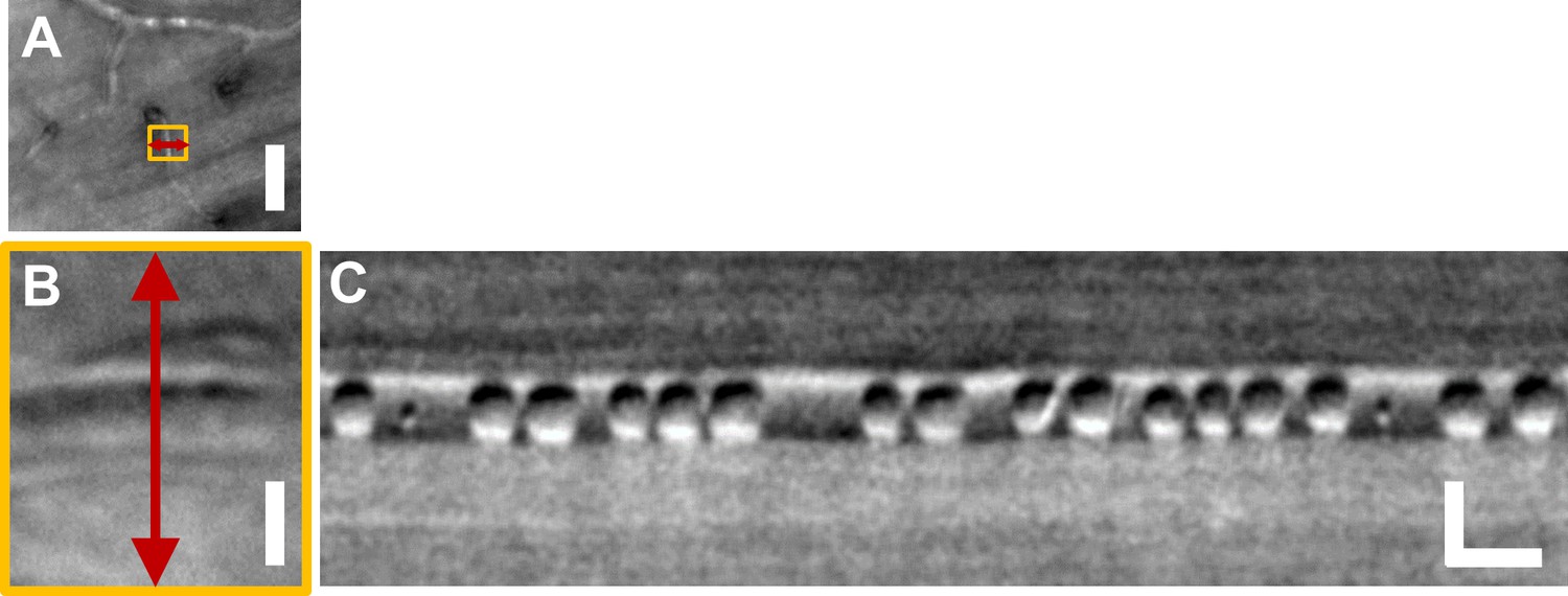
Label-free imaging of single blood cell flux in capillaries.
(A) Cartesian image showing imaged capillary in yellow box. Imaged with 796∆17 nm split-detection AOSLO imaging. Scale bar: vertical = 30 µm (B) Zoomed-in version of yellow box in A, rotated by 90°, clearly showing imaged capillary. Red double-arrow shows line-scan location, similar to Figure 1B. 1D line-scan is placed orthogonal to capillary to image blood cell flux, unlike the oblique scanning shown in Figure 1B when imaging velocity in larger vessels. Scale bar: vertical = 4 µm (C) Space-time image collected at 15 kHz 1D scan rate shows individual blood cells imaged label-free. Scale bars: horizontal = 10 ms, vertical = 4 µm. Please refer to our detailed study on label-free measurement of cell flux in mouse retinal capillaries in Guevara-Torres et al. (2016).
Figure 2
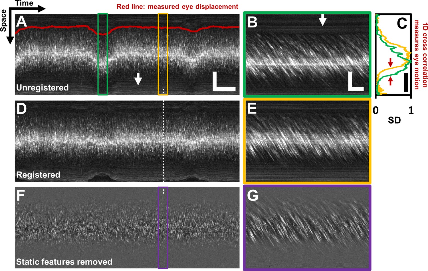
Registration of space-time image and removal of ‘static’ features.
(A) A one second long raw space-time image from the vessel in Figure 1. Actual image is 608 × 15063 pixels across. Eye motion (due to respiration etc.) causes vessel lumen position to change, as observed in image, making laminar profile measurement challenging if eye motion is not corrected for. For visualization, especially of the static features, image brightness of A–E has been increased by 20%. Scale bars: horizontal = 100 ms, vertical = 40 µm (B) A sample target image, 40 ms long, which is a zoomed-in version of green box in A. For each line in A, information from a symmetric 40 ms window around it is used as the ‘target’ for eye-motion registration. Scale bars: horizontal = 5 ms, vertical = 40 µm. (C) Standard deviation (SD) of pixel values in time dimension (or ‘motion contrast’), is plotted as a function of spatial coordinate. Scale bar: 40 µm. Green and yellow plots correspond to SD profiles of B and E respectively. To register all time points to the same reference lumen position, 1D normalized cross-correlation between SD profiles of target image and a user-defined reference image is used. Thus, eye displacement along fast-scan direction is quantified for each time-point (each line) in space-time image in A. Measured eye motion trace is overlaid on same spatial scale in A (dark red line). This eye motion trace is compared to blood cell velocity trace (measured from same space-time image) later. (D) Registered version of space-time image in A. (E) A 40 ms long reference image, which is a zoomed-in version of yellow box in A. (F) Background subtracted version of image in D. White arrows in A and B shows ‘static’ features (retinal tissue outside lumen) which move much slower than blood cells do. These static features may interfere with slope measurement of moving blood cells. Therefore, a moving-average window of 10 ms is used to subtract the background, leaving only moving blood cells in the image. (G) Background-subtracted version of E. Near horizontal lines due to vessel side-walls, other retinal tissue and specular reflection from top of the vessel have been suppressed.
Figure 3
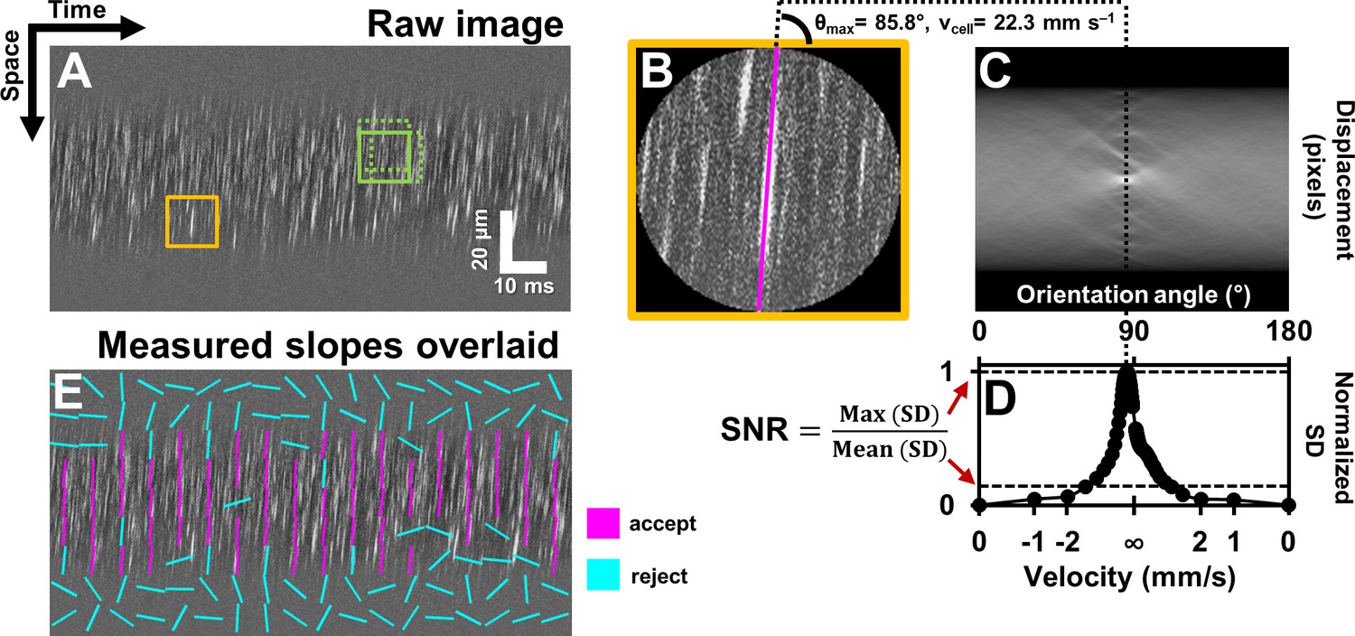
Automated measurement of blood velocity using Radon transform.
(A) A 110 ms long space-time image of a 23.3 µm arteriole scanned obliquely, with static features removed, as described in Figure 2. Solid yellow box shows a square ROI of side 157 pixels (~15 µm x 10 ms) used to inspect single-cell velocity. Dashed green boxes show typical 75% overlap of inspection ROIs. (B) Zoomed-in version of solid yellow box in A. The ROI is circularly cropped to make the interpretation of the Radon transform easier. (C) Radon transform of the ROI in B. Local maxima in pixel intensity correspond to individual blood cell streaks in the single ROI in B. (D) Normalized standard deviation (SD) of pixel values of Radon image in C plotted as a function of orientation angle. The horizontal axis is shown both in angle space and corresponding velocity space (angle to velocity mapping given by Equation 1). Angle corresponding to peak of variance profile in D gives dominant orientation and velocity of streaks in single ROI in B. Measured cell orientation is overlaid as magenta line in B. The cell was moving at 22.3 mm s–1. To determine strength/believability of velocity measurement, a custom signal-to-noise-ratio (SNR) metric is defined as the peak standard deviation (SD) divided by the mean SD. (E) Space-time image in A with measured cell orientations in each ROI overlaid using straight lines. For visualization, only a subset of ROIs are displayed, with no overlap. Magenta lines represent ROIs which passed the custom defined SNR threshold (SNR >2.5). Notice that the magenta lines consistently report a tight range of orientation angles, as expected from normal physiology in such a small time epic. Meanwhile, cyan lines often correspond to measured orientations which seem to incorrectly report actual cell orientations, thus showing that the SNR threshold does a good job separating signal from noise. Such dense reporting of single-cell velocity enables measuring subtle fluctuations in velocity due to laminar profile and cardiac pressure wave. Velocities corresponding to measured cell orientations are displayed on a colormap, as shown in Figure 4.
Figure 4 with 1 supplement
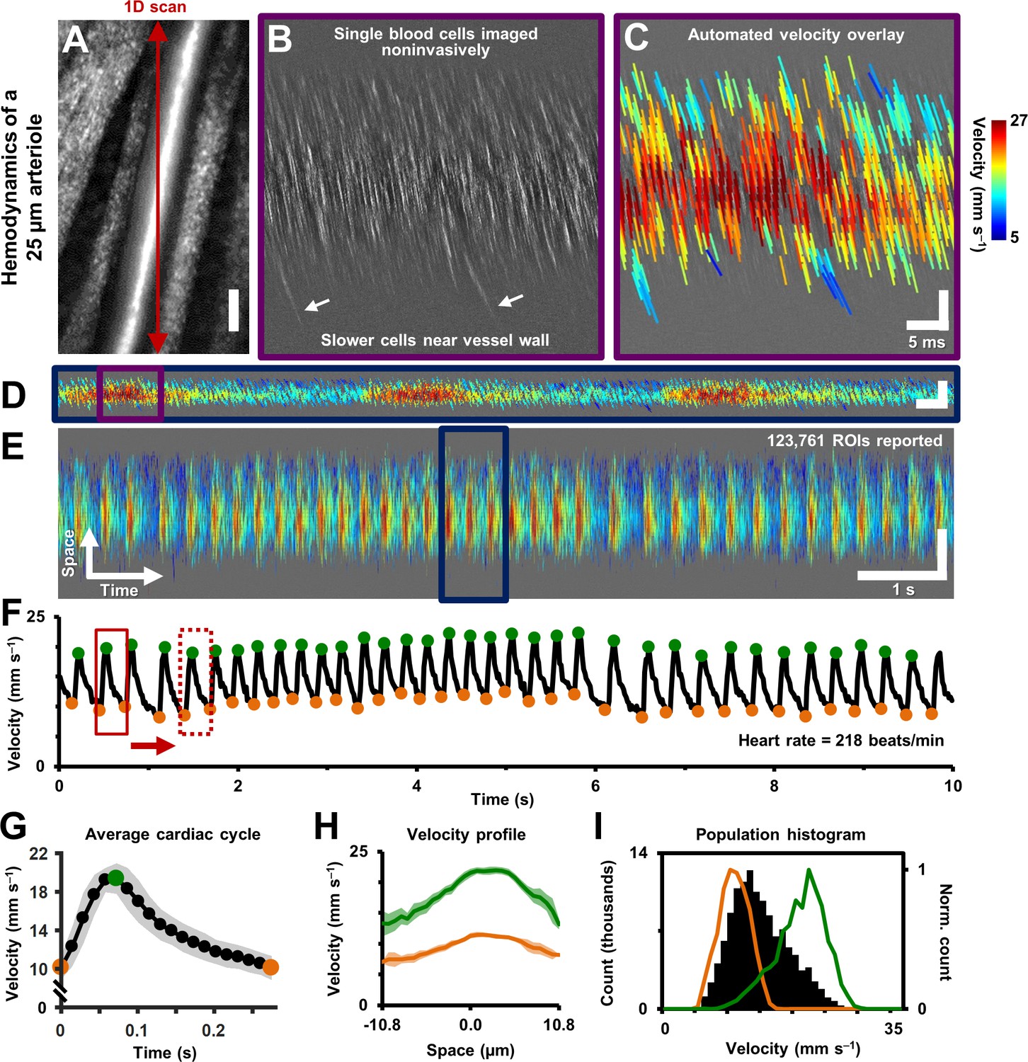
Single-cell hemodynamics of a 25.3 µm retinal arteriole, measured in vivo and noninvasively.
(A) Cartesian image of an arteriole. Dark red arrow marks position of fast 1D oblique scanning. Scale bar: 20 µm. (B) Space-time image showing single blood cells, imaged with 796 nm direct backscatter. White arrows show slower blood cells near vessel wall. For visualization only, image contrast increased by 40%. (C) Automatically measured slopes of cell streaks overlaid on space-time image from B. Color shows absolute cell velocity. Algorithm successfully measured local variations in velocity, including slower cells near vessel wall, marked by white arrows in B. Scale bars: vertical = 20 µm, horizontal = 5 ms. (D) Zooming out: space-time image showing ~711 ms of data in the same vessel, with velocity overlaid in color, spanning ~3 cardiac cycles. Time epoch in C is marked with purple box in D. Scale bars: space: 100 µm, time: 25 ms. (E) Further zooming out: space-time image showing 10 s of data in same vessel. Time epoch in D is marked with dark blue box in E. Several cardiac pulses can be seen (n = 35). Automated algorithm measured single-cell velocity in 123,761 overlapping analysis regions (ROIs). Videos 2 and 3 show all ROIs across 10 s with single-cell detail. Scale bars: space: 50.5 µm, time: 1 s. (F) Instantaneous velocity vs time: cell velocity data was binned across all space and over a 15 ms time window. Putative systolic (green) and diastolic (orange) points shown. (G) High SNR ‘average’ cardiac cycle, which shows highly repetitive pulse waveform, with an asymmetry in time (n = 35 cardiac cycles). Averaging window shown with red boxes in F. Shaded region represents mean ± SD. Figure 4—figure supplement 1 compares this plot to the average cardiac cycle of a similar sized venule. (H) Cross-sectional velocity profile at systolic and diastolic cardiac phases, marked by green and orange time points in G. A blunted parabolic profile is observed, different from prediction of Poiseuille/parabolic flow (vessel lumen diameter = 25.3 µm). Bluntness index of velocity profile changed with cardiac phase (Bsystolic = 1.67, Bdiastolic = 1.39). Shaded regions represent mean ± SD. (I) Population histogram of all the raw velocity data in E, from 123761 ROIs (in black). Overlaid in color are normalized histogram of cell velocities in all diastolic (orange) and systolic (green) phases.
Figure 4—figure supplement 1
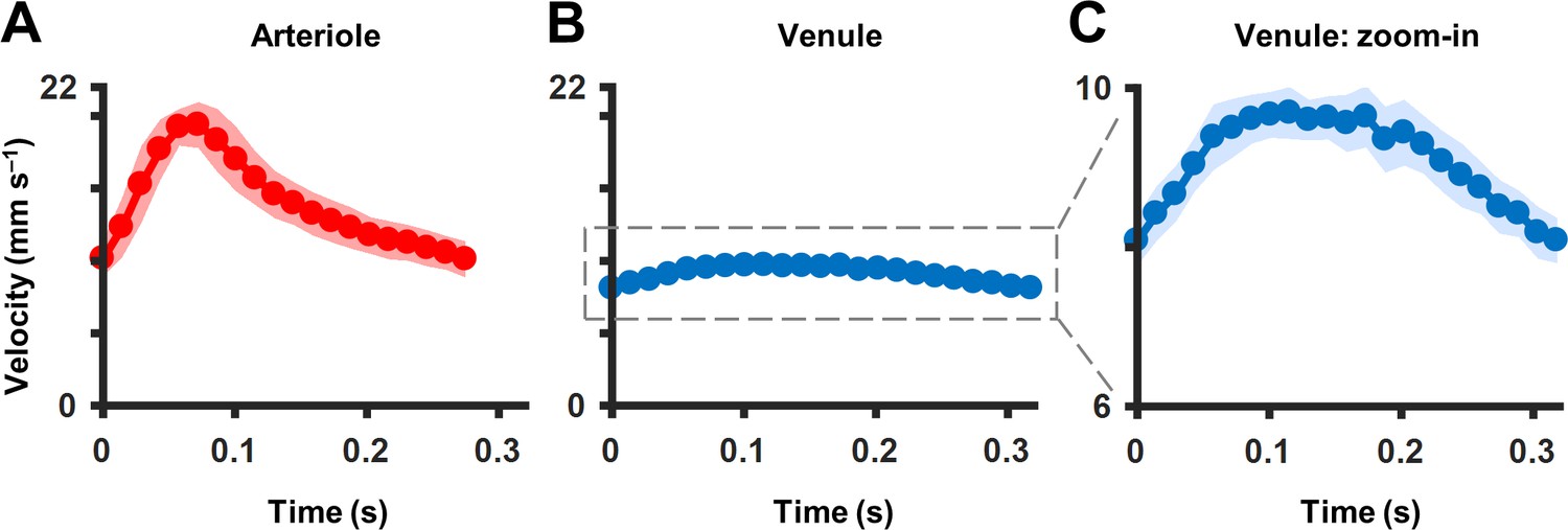
Comparison of average cardiac cycle in an arteriole and venule.
(A) Cardiac waveform from averaging n = 35 cardiac cycles of a 25.3 µm first-generation arteriole (as shown in parent Figure 4G). Pulsatility index (PI) = 0.67 and asymmetry index (AI) = 2.8. (B) Cardiac waveform from averaging n = 29 cycles of a 33.5 µm first-generation venule, shown in the same scale as in A. PI = 0.18 and AI = 1.75. (C) Zoomed-in version of B showing difference in temporal asymmetry of cardiac waveform in venule compared to that of arteriole in A. All shaded regions in plots represent mean ± SD.
Figure 5
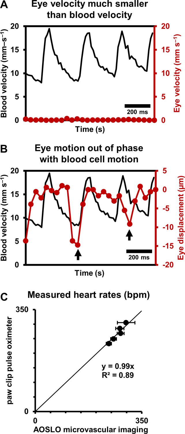
Eye motion minimally affects pulsatile blood velocity measurements.
(A) Comparison of simultaneously measured eye velocity and pulsatile blood velocity (both along fast scan direction). Maximum eye velocity was 23 times smaller than minimum velocity of blood cells, showing that error in blood velocity measurement is less than 4.3%. Data from same vessel as shown in Figure 2 and Figure 4 (B) Comparison of eye displacement with pulsatile blood velocity. Black arrows point towards two time points when the phase of blood cell motion and eye motion are markedly different, showing that the measured periodicity in blood cell motion is not due to any type of periodic eye motion. (C) Comparison of heart rates measured by AOSLO retinal microvascular imaging and simultaneous paw-clip pulse oximeter (Physiosuite Kent Scientific) measurements. Each data point is a unique vessel imaged for 1 s. Error bars represent standard deviation in instantaneous heart rate (AOSLO) measured in a pulse-by-pulse basis (n = 2 to 4 pulses).
Figure 6

Measurement of cross-sectional velocity profile of a vessel only a few times larger than an RBC.
(A) Measured flow profile, averaged over all cardiac phases in 10 s of data, from the arteriole in Figure 4 (lumen diameter = 25.3 µm, typical RBC size = 6.7 µm). Profile is a flattened bell-shaped curve, in contrast to predictions of parabolic/laminar profile from Newtonian law. Slight asymmetry is observed (peak velocity is 1.5 µm away from the assigned zero position of vessel, based on the farthest cell velocities that could be reliably measured). A small gap (1.8 µm) between the known lumen diameter and the RBC column is observed, predicted to arise from the known cell-free regions near the vascular wall. Shaded region represents mean ± SD, where variation is across all ROIs in a 10 s window. Number of ROIs analyzed varied from 7333 in the lumen center to 217 near the vessel wall. (B) Assuming symmetric flow, models are fit to the measured flow profile of this vessel. The flatness of the curve is quantified using Equation 7 (blue line, Zhong et al., 2011) (bluntness index B = 1.51, scale factor β = 0.44). A parabolic profile (red line) would have B = 2 and β = 0. The plasma velocity is extrapolated using a linear-decline model (yellow line), to satisfy the no-slip boundary condition at the vascular wall. The bottom table shows that calculation of mean flow rate in the vessel using only centerline velocity and an assumption of parabolic flow profile results in a 39% underestimation of flow, underlining the importance of direct measurement of velocity profiles in vessels this small, and not relying only on models of flow.
Figure 7
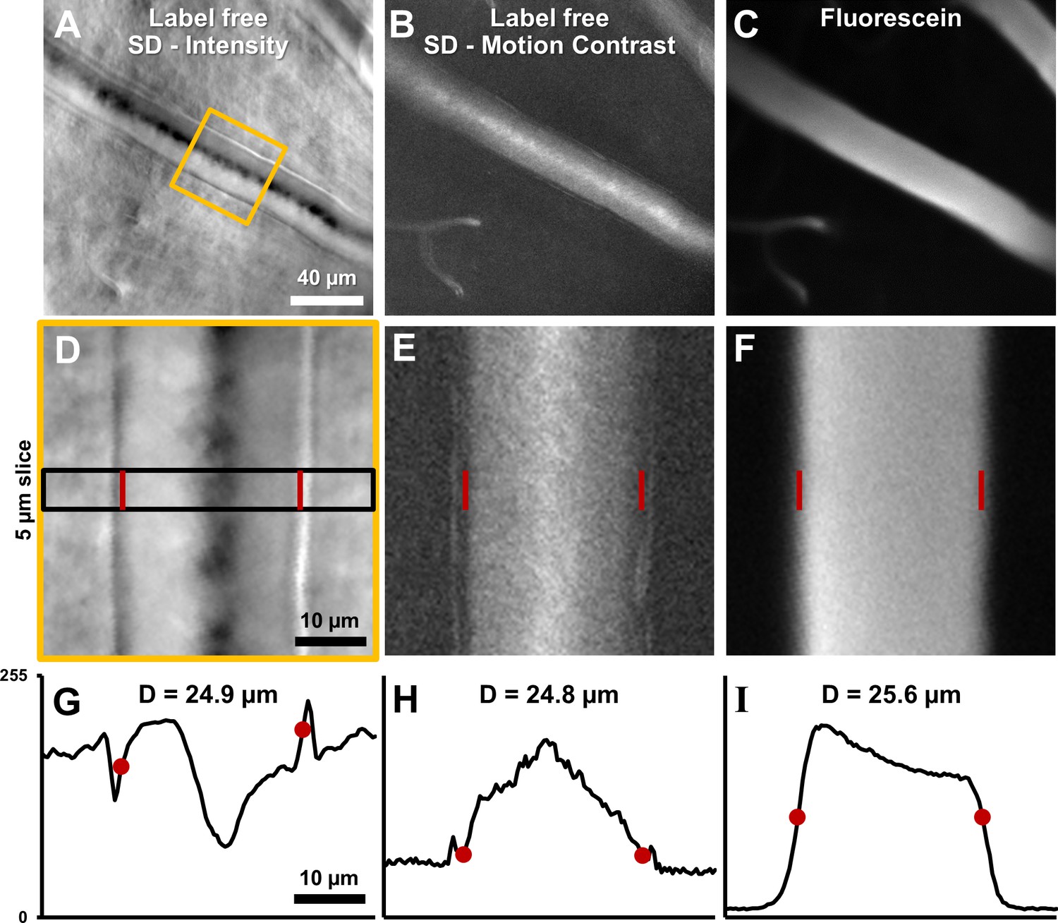
Label-free lumen diameter measurement of microvessel matches conventional fluorescein measurement of the same (both modalities simultaneously collected).
(A) Average intensity image of an arteriole using label-free split detection modality. (B) Motion contrast image (temporal standard deviation of pixel values) obtained from eye-motion corrected video from A. Bright pixels show regions of blood cell motion, clearly outlining the lumen of these tiny microvessels. (C) Flourescien image of same vessel collected simultaneously. (D–F) Zoomed-in images corresponding to yellow box in A, all at the same scale. Radon transform was used to accurately rotate the vessel with its length (and therefore, flow direction) vertical. The vascular wall is clearly seen in D. The side bands in E likely correspond to uncorrected/residual motion of the vascular wall corresponding to respiration/cardiac motion. (G–I) 1D intensity profiles in the three modalities computed in a 5 µm slice (shown by black rectangle in D. The lumen boundaries are marked with red circles in G–I and red bars in D–F. Details of these objective measurements are given in manuscript’s text. Lumen diameters match across modalities, with errors within 3%. The slightly larger fluorescein diameter is likely attributed to fluorescein representing true lumen width while split-detection motion contrast represents the RBC column width, not including the cell-free zone near vessel walls.
Figure 8
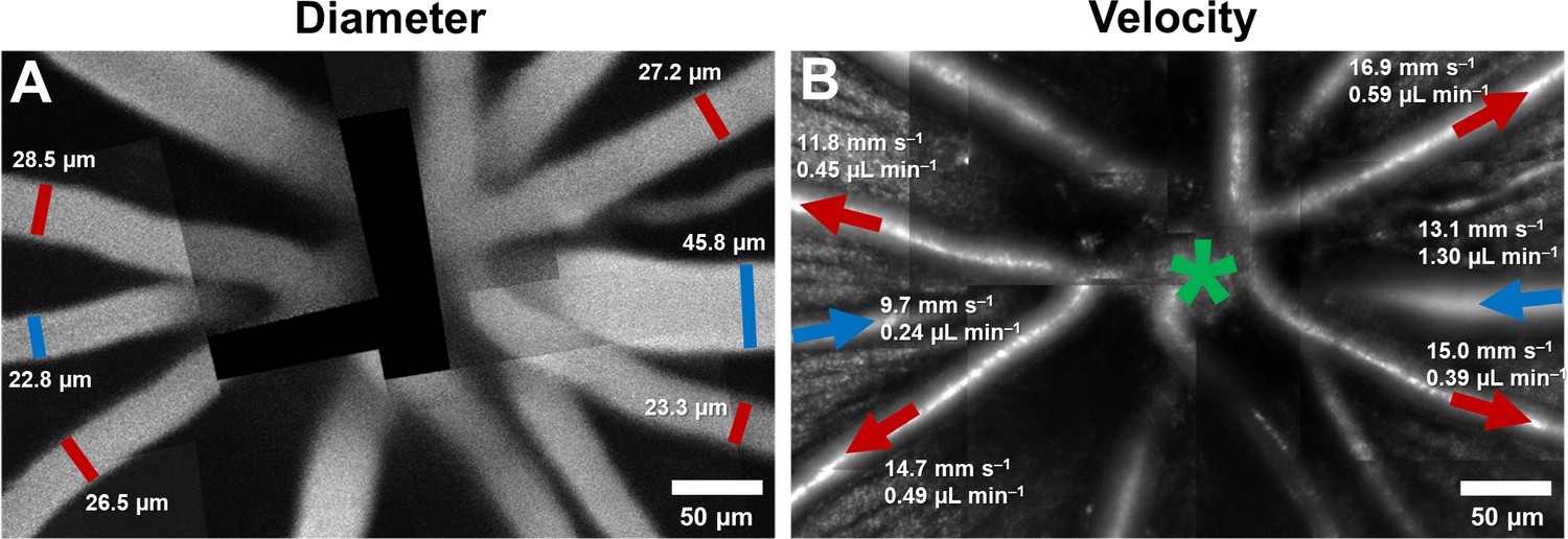
Montage of multiple AOSLO fields showing hemodynamics in primary vessels radiating from the optic disk in one mouse.
(A) Montage of fluorescein images. (B) Montage of infrared reflectance images at same retinal location. Green star marks center of optic disk. Lumen diameter and mean flow rate are reported for each analyzed vessel. Arrows point towards direction of flow. Red color represents arterioles and blue, venules.
Figure 9

Functional mapping of hemodynamics across five vessel generations in the retina.
(A) Montage of multiple AOSLO imaging fields showing structure of the mouse retinal vascular tree. The center of the optic disk is marked with a green star. Arterioles in which flow was studied in this mouse are shown with red arrows: A1 (2nd gen), A2 (4th gen.), A3 (5th gen.) and A4 (5th gen.). Blue arrow shows a 1st gen. venule (V1) adjacent to this arteriolar branch. All arrows point toward direction of blood flow. (B) Quantification of conservation of flow at a branch point, in the vessels A2, A3 and A4. Flow is conserved within a < 8.9% error, validating our technique’s measurement accuracy in these independent measures made within minutes of each other. (C) Instantaneous velocity vs time plots for the vessels labelled in A. (D) Instantaneous flow rate vs time profiles, derived by multiplying each profile in B with the lumen diameter of the vessel. In summary, a functional map across five vessels generations in the same mouse is shown, showing temporal dynamics of microvascular blood flow.
Figure 10
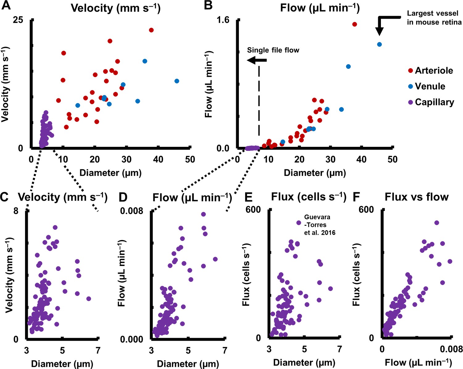
Hemodynamics in complete spectrum of retinal vessel sizes in population of vessels (in 19 normal C57BL6/J mice, across 123 vessels: 25 arterioles, 8 venules and 90 capillaries across all vessel generations in retina).
(A) Mean velocity vs lumen diameter in all vessels. Heterogeneity in velocity is observed across the spectrum (for arbitrary linear fits on velocity-diameter relationship, arteriole: R2 = 0.31, venule: R2 = 0.43, capillary: R2 = 0.21). (B) Mean flow rate vs lumen diameter in all retinal vessels, from single-file-flow capillaries to the largest vessel near optic disk in mouse retina. Inclusion of diameter in flow calculation induces strong dependence of flow rate on diameter (for power fit, arterioles: exponent = 2.56, R2 = 0.86, venules: exponent = 2.49, R2 = 0.96). Murray’s theoretical model for blood vessels predicts a cubic relationship between flow rate and diameter. (C–D) Zoom-in of velocity and flow rate vs diameter for capillaries only (n = 90 capillaries). The linear vertical axis in B prevented the visualization of the near four orders of magnitude range of blood flow rates measured. Wide heterogeneity is observed, with weak correlation of capillary velocity and flow rate with lumen diameter (for arbitrary linear fit, velocity vs diameter: R2 = 0.21, flow vs diameter: R2 = 0.61). (E) Data from label-free measurements of single-cell flux in capillaries reported in our previous publication, reproduced here for 90 vessels. (F) Correlation of measured flux and flow rate in the same 90 single-file-flow capillaries (linear fit, R2 = 0.79). The spread in the data represents variations in discharge hematocrit due to plasma skimming. Thus, in single-file-flow vessels (i.e. capillaries), measurement of velocity and flow alone gives an incomplete picture of nutrient delivery; cell flux gives a more accurate picture of the same.
Figure 11
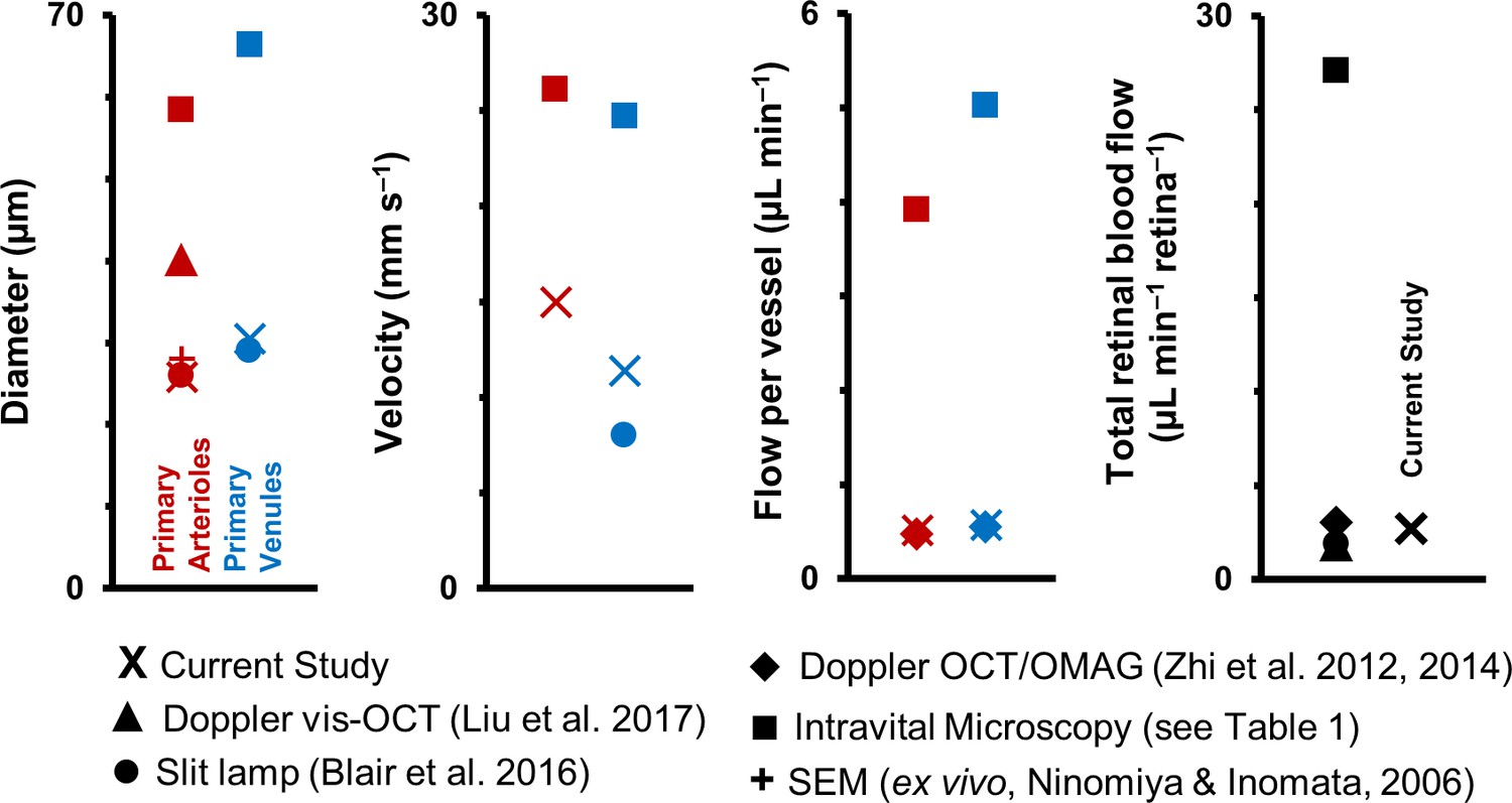
Graphical representation of data in Table 1.
Previous studies of retinal blood vessel diameter, mean velocity and mean flow in first-generation (or ‘primary’) vessels radiating out of optic disk in normal mice. Wide disparity is observed across studies. (Note: Values for Intravital Microscopy are averaged from Wright et al., 2012; Yadav and Harris, 2011; Wang et al., 2011; Wang et al., 2010; Wright et al., 2009; Lee and Harris, 2008) and Wright and Harris, 2008).
Videos
Video 1
Video of a first-generation arteriole (25.3 µm) emerging from the optic disk of a mouse, imaged at conventional 25 Hz frame rate using a raster scanning AOSLO.
The fast-scan (15 kHz) is in the horizontal direction and slow (25 Hz) in the vertical direction. Direct backscatter is imaged using a 796∆17 nm super-luminescent diode (~500 µW). Single blood cells can be seen passing as bright streaks within the lumen of the vessel. However, frame-rate of 25 Hz is too slow to quantify the velocity of these fast moving blood cells without aliasing or missing cells. To overcome this problem, 1D scanning is performed at the vessel at 15 kHz to form space-time images of blood cell motion, as shown in Figure 1 . The video is 10 s long and has dimensions of 4.80° x 3.73° (163.2 × 126.8 µm). The video has been corrected for eye motion as described in the paper. The 250 frames in this video were averaged to form the high SNR image of the same vessel shown in Figure 1B.
Video 2
All 10 s of high-resolution data of single-cell blood flow captured in the 25.3 µm arteriole shown in Figure 4.
Top: Raw space-time image. Bottom: Cell slopes and velocity overlaid on the original space-time image. N = 35 unique cardiac cycles shown. Scale bars: 4 ms (horizontal), 20 µm (vertical).
Video 3
Blood velocity profile across 20 cardiac phases imaged noninvasively in a 25.3 µm arteriole.
Top: Space-time image (10 s) of the 25.3 µm arteriole shown in Figure 4. Image is overlaid with measured absolute single-cell velocity, as described in the paper. Scale bars: 300 ms (horizontal), 60 µm (vertical). Middle: Zoom-in of purple box, showing a single representative cardiac pulse in the space time image. Scale bars: 10 ms (horizontal), 25 µm (vertical). Bottom-left: A ~ 12 ms window of the space-time image (red box) is shown in both raw form (showing single blood cell streaks) and in velocity overlaid form. Scale bars: 3 ms (horizontal), 10 µm (vertical). Bottom right: The first plot shows an average cardiac cycle computed from n = 35 cycles, same as Figure 4G. The second plot shows the velocity (spatial) profile as a function of cardiac phase. Figure 4H had only shown the diastolic and systolic phases. The bluntness and height of the profile can be observed to change with cardiac phase. Bluntness index (B) and relative height of profile edges (β) were quantified using Equation 7 in the paper. Bsystolic = 1.67, Bdiastolic = 1.39, βsystolic = 0.34, βdiastolic = 0.46. Shaded regions in both plots show mean ± SD.
Tables
Table 1
Previous studies of vessel diameter, mean velocity and mean flow rate in first-generation retinal blood vessels radiating out of optic disk in normal mice.
Wide disparity in measured values is observed across studies. Figure 11 graphically summarizes differences across studies. Abbreviations: Nm: number of mice, Nv: number of vessels, D: Mean diameter of vessels, Vm: Mean velocity per vessel, Fm: Mean flow rate per vessel, TRBF: total retinal blood flow per mouse (calculated by summing flow from all primary arterioles/venules around optic disk), A: primary arterioles, V: primary venules, SD: standard deviation, NOD: Non-obese diabetic. Special markers: ^ Assuming 3–7 primary arterioles and venules each per mouse retina. * SD represents variation across mice and not across vessels. An average arteriolar and venular value was calculated first for each mouse. # values represent mean ± standard error of mean. Variation is across mice and not across vessels. a: Values are mean ± SD, where SD represents variation across vessels, and not mice. Value ranges mentioned in brackets. Measurements in the current study were performed on primary retinal arterioles and venules radiating out of optic disk, at locations within a ~170–300 µm radius from the center of the optic disk. a1: Estimated by multiplying the measured Fm per vessel with the number of vessels per retina. Assumed 3–7 primary arterioles and venules per retina. b: Mean velocities are not reported here as it is unclear if the velocities reported in that study represent the mean or the sum of the individual vessel velocities per retina. c: Variation in Fm per vessel represents variation (SD) across six vessels. Variation in total flow represents variation across three independent measurements. d: Numbers correspond to diameter measurements only. For velocity measurements, Nm = 5–13, Nv = 27–71.
| Study | Technique | Species | Class | Nm | Nv | D (µm) | Vm (mm s–1) | Fm per vessel (µL min–1) | TRBF (µL min−1retina−1) |
|---|---|---|---|---|---|---|---|---|---|
| Current study | Adaptive optics line-scan | 15–73 week old C57BL/6J mice | A | 7 | 11 | 25.9 ± 4.6 a (20.1–37.7) | 15.0 ± 4.0 a (9.9–23.1) | 0.52 ± 0.36 a (0.22–1.55) | 1.56–3.64 a1 |
| V | 6 | 7 | 30.6 ± 8.4 a (22.8–45.8) | 11.4 ± 3.0 a (8.6–17.0) | 0.57 ± 0.42 a (0.24–1.30) | 1.71–3.99 a1 | |||
| Liu et al., 2017 | Dual ring scanning Doppler vis-OCT | 13 week old non-diabetic TSP1-/- mice | A | 7 | 21–49 ^ | 40.1 ± 1.8 * | - b | - | 1.86 ± 0.24 * |
| V | 7 | 21–49 ^ | - | - | - | - | |||
| Blair et al., 2016 | Slit lamp biomicroscope | 24 week old C57BL/6J mice | A | 10 | 30–70 ^ | 26 ± 2 * | - | - | - |
| V | 10 | 30–70 ^ | 29 ± 3 * | 8 ± 1 * | - | 1.9 ± 0.5 * | |||
| Zhi et al., 2014 | En face Doppler OCT/OMAG | BTBR wild-type mice | A/V | 10 | 30–70 ^ | - | - | - | 3.05 ± 0.20 # |
| Wright et al., 2012 | Intravital microscopy | 30–31 week old male C57BL/6J mice | A | 9 | 45 | 57.3 ± 1.1 # | 25.3 ± 1.3 # | 4.02 ± 0.28 # | - |
| V | 9 | 45 | 62.5 ± 2.4 # | 23.2 ± 1.1 # | 4.83 ± 0.41 # | - | |||
| Zhi et al., 2012 | En face Doppler OCT/OMAG | 22 week old female BTBR mice | A | 1 | 6 | - | - | 0.47 ± 0.05 c | 2.82 ± 0.30 c |
| V | 1 | 6 | - | - | 0.55 ± 0.10 c | 3.27 ± 0.28 c | |||
| Yadav and Harris, 2011 | Intravital Microscopy | 16 week old male C57BL/6 mice | A | 12 | 36–84 ^ | 60.0 ± 1.3 # | 30.2 ± 1.4 # | 5.29 ± 0.34 # | - |
| V | 12 | 36–84 ^ | 67.6 ± 1.6 # | 28.0 ± 1.2 # | 6.39 ± 0.31 # | - | |||
| Wang et al., 2011 | Intravital microscopy | 13 week old male C57BL/6 mice | A | 7 | 21–49 ^ | 56.0 ± 1.1 # | 29.0 ± 0.8 # | - | - |
| V | 7 | 21–49 ^ | 66.4 ± 2.8 # | 25.1 ± 0.7 # | - | 25.08 ± 1.92 # | |||
| Wang et al., 2010 | Intravital microscopy | 13–14 week old male C57BL/6 mice | A | 6 | 30–42 | 54.7 ± 1.0 # | 20.9 ± 0.7 # | 2.98 ± 0.14 # | - |
| V | 6 | 30–42 | 60.8 ± 2.7 # | 21.0 ± 0.7 # | 3.86 ± 0.36 # | - | |||
| Wright et al., 2009 | Intravital microscopy | 15–16 week old male C57BL/6 mice | A | 7–8 | 28–49 | 59.4 ± 0.9 # | 28.3 ± 1.4 # | - | 26.34 ± 2.52 # |
| V | 7–8 | 28–49 | 69.5 ± 1.4 # | 26.3 ± 1.2 # | - | 31.80 ± 2.40 # | |||
| Lee and Harris, 2008 | Intravital microscopy | 16–30 week old female euglycemic NOD mice | A | 5 | 9–13 | 61.0 ± 1.5 # | - | 3.36 ± 0.18 # | - |
| V | - | - | - | - | - | - | |||
| Wright and Harris, 2008 | Intravital microscopy | 16 week old C57BL/6 mice | A | 7–9 d | 41–50 d | 60.4 ± 1.1 # | 23.0 ± 0.5 # | - | - |
| V | 7–9 d | 37–49 d | 71.4 ± 2.9 # | - | - | - | |||
| Ninomiya and Inomata, 2006 | Scanning electron microscopy (ex vivo) | 16 week old male mice | A | 10 | 80 | <28 | - | - | - |
| V | - | - | - | - | - | - |
Key resources table
| Reagent type (species) or resource | Designation | Source or reference | Identifiers | Additional information |
|---|---|---|---|---|
| Strain, strain background (Mus musculus) | C57BL/6J mice | The Jackson Laboratory, Bar Harbor, Maine, USA. https://www.jax.org/strain/000664 | RRID:IMSR_JAX:000664, JAX stock #000664 | |
| chemical compound, drug | AK-FLUOR 10% (100 mg mL–1) | Akorn, Lake Forest, Illinois, USA | NDC: 17478-253-10 | IP injection of 0.1 mL of 2.5% weight/volume |
Additional files
-
Supplementary file 1
The number and type of mice used in each figure.
Our study is focused on (1) the method and (2) generating a novel dataset of hemodynamics in the healthy mouse. As such, Figures 1–9 are designed to show the method and analysis steps, algorithm validation and representative examples of measurements made. Therefore, these figures typically show one or a few vessels, from one mouse, unless otherwise mentioned in the table above. The population data across all mice imaged is shown in Figure 10. Population data are reported for mean velocity, flow, diameter and flux, across multiple mice, as quantified in the table above.
- https://doi.org/10.7554/eLife.45077.020
-
Supplementary file 2
Raw space-time image corresponding to top-half of Video 2.
- https://doi.org/10.7554/eLife.45077.021
-
Supplementary file 3
Cell slopes and velocity overlaid on the original space-time image in Supplementary file 2.
N≈three unique cardiac cycles shown.
- https://doi.org/10.7554/eLife.45077.022
-
Transparent reporting form
- https://doi.org/10.7554/eLife.45077.023
Download links
A two-part list of links to download the article, or parts of the article, in various formats.
Downloads (link to download the article as PDF)
Open citations (links to open the citations from this article in various online reference manager services)
Cite this article (links to download the citations from this article in formats compatible with various reference manager tools)
Imaging single-cell blood flow in the smallest to largest vessels in the living retina
eLife 8:e45077.
https://doi.org/10.7554/eLife.45077


