Inference of nonlinear receptive field subunits with spike-triggered clustering
Figures
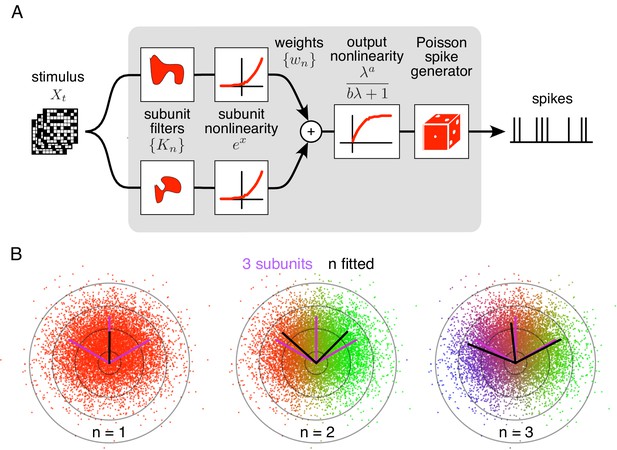
Spiking response model, and estimation through spike-triggered stimulus clustering.
(A) The model is constructed as a cascade of two linear-nonlinear (LN) stages. In the first stage, subunit activations are computed by linearly filtering the stimulus () with kernels () followed by an exponential nonlinearity. In the second stage, a sum of subunit activations, weighted by (), is passed through a saturating output nonlinearity (), yielding a firing rate that drives an inhomogeneous Poisson spike generator. (B) Estimation of subunits in simulated three-subunit model cell. Responses are generated to two-dimensional Gaussian stimuli (iso-probability circular contours shown) with three subunits (magenta lines), generating a spike-triggered stimulus ensemble (colored dots). Weights for different subunits are assigned to each spike triggered stimulus, with colors indicating the relative weights for different subunits. Subunits are then estimated by weighted summation of spike triggered stimulus ensemble (black lines). Soft-clustering of spike triggered stimuli with different number of clusters results in progressive estimation of the underlying subunits. Clustering with correct number of subunits (right panel) results in estimated subunits (black lines) aligned with the true subunits.
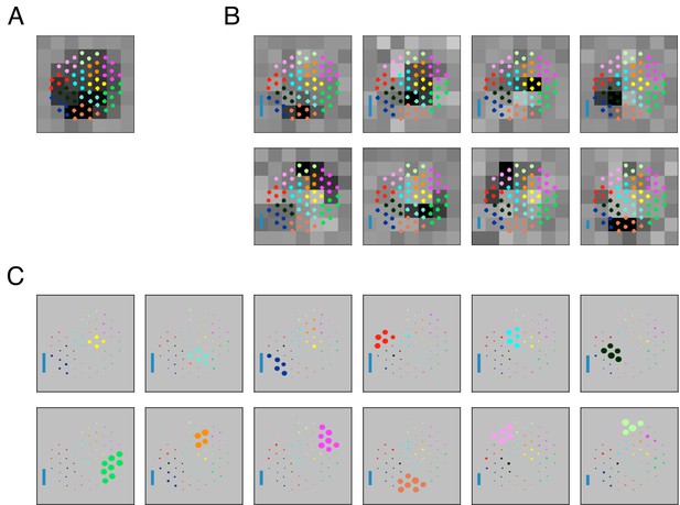
Validation of the subunit fitting algorithm on simulated RGC data.
(A) Receptive field obtained via spike-triggered average of a simulated RGC with cascaded linear nonlinear units. The stimulus is temporally filtered by 64 photoreceptors organized on a jittered hexagonal grid. Inputs from 4 to 8 photoreceptors are summed by each of 12 bipolar cells. Bipolar activations are exponentiated and added to produce the firing rate, and spikes are generated by sampling from a Poisson process. Dots indicate photoreceptor locations, with color indicating photoreceptors connecting to a common bipolar cell. See Materials and methods for further details. (B) Subunits estimated from simulated RGC responses to coarsely-pixelated white noise reveals fewer subunits (8) than the actual number of bipolar cells (12). The estimated subunits are spatially localized, and partially overlapping (corresponding to weighted aggregates of adjacent underlying bipolar cells), and together cover the receptive field. Inset: Blue bar height indicates the relative strength (average contribution to response over the stimulus ensemble) of each subunit (see Equation 6 in Materials and methods). (C) Subunits estimated from simulated RGC responses to a white noise stimulus in which the individual elements of the stimulus target individual cones. The simulation correctly recovers 12 subunits (cross-validated), in which the groups of cones correspond to those that feed each of the simulated bipolar cells. Sizes of dots indicate relative weights of different photoreceptors to the estimated subunits. Inset: Same as B.
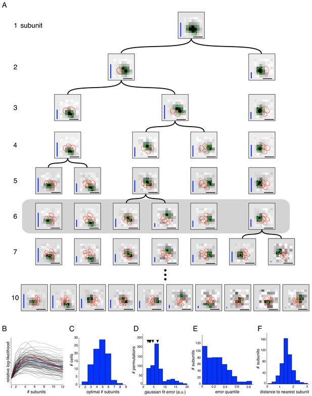
Estimated subunit properties.
(A) Subunits, shown as grayscale images, estimated from OFF parasol cell responses to 24 min of white noise. Each pixel was temporally prefiltered with a kernel derived from the spike-triggered average (STA). Rows show estimated spatial subunits for successive values of N. Subunit locations are indicated with ellipses (green for same subunit, red for other subunits from the same fit), corresponding to the contour of a fitted two-dimensional Gaussian with standard deviation equal to the average nearest neighbor separation between subunits. As N increases, each successive set of subunits may be (approximately) described as resulting from splitting one subunit into two (indicated by lines). Large N (e.g. last row) yields some subunits that are noisy or overlap substantially with each other. Height of vertical blue bars indicate the relative strength (average contribution to the cell's firing rate over stimulus ensemble, ignoring the output nonlinearity) of each subunit (see Equation 6 in Materials and methods). Horizontal black bars indicate spatial scale (150μm). (B) Log-likelihood as a function of number of subunits (relative to single subunit model) for 91 OFF parasol cells (black) on 3 min of held-out test data, averaged across 10 random initializations of the model, from a distinct randomly sampled training data (24 min from remaining 27 min of data). Population average is shown in blue and the example cell from (A) is shown in red. (C) Distribution of optimal number of subunits across different cells, as determined by cross-validated log-likelihood on a held-out test set for OFF parasol cells. (D, E) Spatial locality of OFF parasol subunits, as measured by mean-squared error of 2D gaussian fits to subunits after normalizing with the maximum weight over space. Control subunits are generated by randomly permuting pixel weights for different subunits within a cell. For this analysis, the optimal number of subunits was chosen for each cell. (D) Distribution of MSE values for randomly permuted subunits for the cell shown in (A). MSE of six (optimal N) estimated subunits indicated with black arrows. (E) Distribution of quantiles of estimated OFF parasol subunits, relative to the distribution of MSE values for permuted subunits, across all cells and subunits. Null hypothesis has uniform distribution between 0–1. (F) Distribution of distances to nearest neighboring subunit within each OFF parasol cell. Distances are normalized by geometric mean of standard deviation of the gaussian fits along the line joining center of subunits. For this analysis, each cell is fit with five subunits (most frequent optimum from (C)).
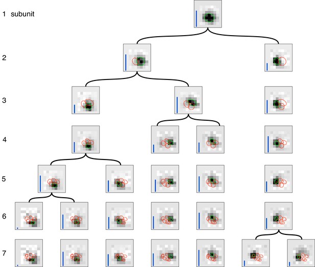
Gradual partitioning of the receptive field into subunits by hierarchical clustering.
Different number of subunits (rows) estimated by splitting one parent subunit into two subunits at each step. Children subunits estimated by soft-clustering the simulated spikes of the parent subunit, with the simulated spikes for parent subunit computed as the spiking activity of the cell, weighed by its soft-max subunit activation (see Materials and methods). The parent subunit that gives maximum decrease in log-likelihood on training data is chosen for splitting. The choice of training data, preprocessing and figure details same as Figure 2. The achieved splitting of subunits is similar to the pattern of splitting in Figure 2 for small number of subunits (1–5 subunits), but differs for larger number of subunits (6, 7 subunits). This suggests that enforcing the hierarchical constraint could lead to a more efficient estimation procedure.
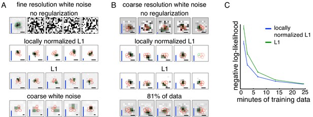
Spatially localized subunit estimation.
Comparison of different regularizers for estimating subunits using limited data. Examples of OFF parasol cells are shown. (A) Five subunits (most frequent optimum across cells from Figure 2) estimated using all data (1 hr 37 min) for fine resolution white noise without regularization (top row). The first estimated subunit is identical to the full receptive field and the others are dominated by noise. Locally normalized L1 (second row) and L1 (third row) regularization both give spatially localized subunits, with L1 regularization leaving more noisy pixels in background. In both cases, optimal regularization strength was chosen (from 0 to 1.8, steps of 0.1) based on performance on held-out validation data. The contours reveal interdigitation of subunits (red lines). Subunits estimated using white noise with 2.5x coarser resolution (24 min) and no regularization are larger, but at similar locations as subunits with fine resolution (bottom row). Height of vertical blue bars indicate the relative strength (average contribution to response) for each subunit (see Equation 6 in Materials and methods). Scale bar: 75 µm (B) For the cell in Figures 1A, 5 subunits estimated using the 3 min (10% of recorded data) of coarse resolution white noise responses are noisy and non-localized (top row). Similar to the fine case, using locally normalized L1 (second row) and L1 (third row) regularization both give spatially localized subunits, with L1 regularization subunits having noisier background pixels. The regularization strength (between 0 and 2.1, steps of 0.1) was chosen to maximize log-likelihood on held out data (last 5 min of data). Subunits estimated using 24 min (81% of data) of data are spatially localized and partition the receptive field (bottom row). Vertical bars same as (A). Scale bar: 150 µm (C) Held out log-likelihood for a 5 subunit model estimated from varying durations of training data with L1 (green) and locally normalized L1 (blue) regularization. Results averaged over 91 OFF parasol cells from Figure 1A.
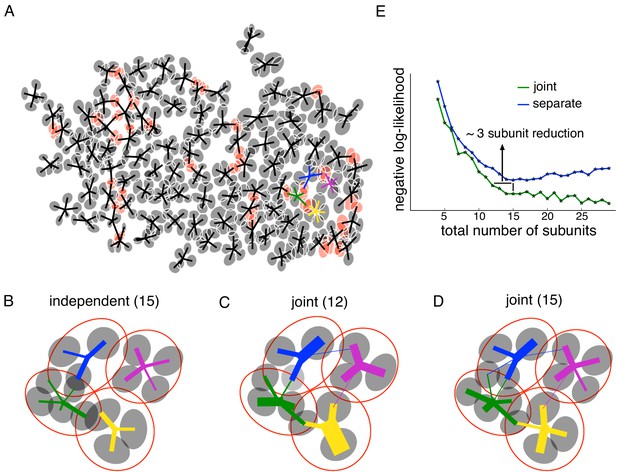
Joint estimation of subunits across multiple nearby cells.
(A) Gaussian fits to the subunits estimated for an entire OFF parasol cell population (5 subunits per cell, with poorly estimated subunits removed). Lines connect center of each cell to its subunits. Subunits which are closer to their nearest neighbor than average (below 15 percentile) are indicated in red. (B) Detailed examination of four neighboring cells from the population (color-coded). Number of subunits for each cell is chosen (total 15 subunits) to give the highest summation of log-likelihood (on validation data) for four nearby cells. Gaussian fits to receptive field of the cells (red) and their subunits (gray). Connection strength from a cell (distinct color) to its subunits is indicated by thickness of line. (C) A common bank of 12 subunits estimated by jointly fitting responses for all four cells gives similar accuracy as (B). Sharing is indicated by subunits connected with lines of different colors (different cells). (D) A model with a common bank of 15 subunits (same number as B) gives better performance than estimating the subunits for each cell separately. (E) The total negative log-likelihood on test data for these four cells (y-axis) v/s total number of subunits (x-axis) for the two population models with subunits estimated jointly across cells (green) and a combination of separately estimated subunits chosen to maximize total log-likelihood on validation data (blue). Horizontal shift between curves indicates the reduction in total number of subunits by jointly estimating subunits for nearby cells for similar prediction accuracy. The vertical shift indicates better performance by sharing subunits, for a fixed total number of subunits. For both separate and joint fitting, the best value for locally normalized L1 regularization (in 0–3, step size 0.2) for a fixed number of subunits was chosen based on the performance on a separate validation dataset (see Materials and methods).
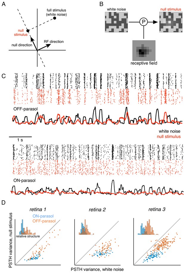
Cells respond to stimulus in null space of receptive field.
(A) Construction of null stimulus, depicted in a two-dimensional stimulus space. Each dimension of stimulus space consists of intensity along a particular pixel. A stimulus frame is represented as a point in this space. Each stimulus frame can be represented geometrically as the sum of the component along the receptive field (RF) direction (the response component of a linear nonlinear model) and the component orthogonal to the RF direction (the null component). (B) The null stimulus is constructed by projecting out the RF contribution from each frame of white noise stimulus. (C) Rasters representing responses for an OFF parasol (top) and ON parasol (bottom) cell to 30 repeats of 10 s long white noise (red) and the corresponding null stimulus (black). (D) Response structure for ON parasol (blue) and OFF parasol (orange) populations for white noise (x-axis) and null stimulus (y-axis) across three preparations (different plots). The response structure was measured as variance of PSTH over time. Variance of PSTH converged with increasing number of trials (not shown), suggesting minimal contribution of inter-trial variability to response structure. Insets: Histogram of relative structure in white noise responses that is preserved in null stimulus for ON parasol (blue) and OFF parasol (orange). Relative structure is measured by ratio of response structure in the null stimulus and response structure in white noise stimulus.
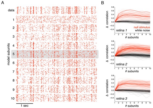
Subunits improve prediction of responses to null stimuli.
(A) Rasters for recorded responses of an OFF parasol cell to 30 presentations of a 5 s long null stimulus (top row). Predictions of models with increasing (1 to 10) number of subunits (subsequent rows). (B) The change in correlation (relative to the correlation obtained with one subunit) between PSTH for recorded and predicted responses with different numbers of subunits across three preparations. Spatial kernels were estimated from 24 min of non-repeated white noise stimulus, with scales and output nonlinearity estimated from the first 5 s of the repeated stimulus. Performance on the last 5 s of the repeated stimulus was averaged over 10 fits, each with a random subsample of the non-repeated white noise stimulus. Individual OFF parasol cells (thin lines) and population average (thick lines) for the null stimulus (red) and white noise (black). The cell in (A) is indicated with dashed lines.
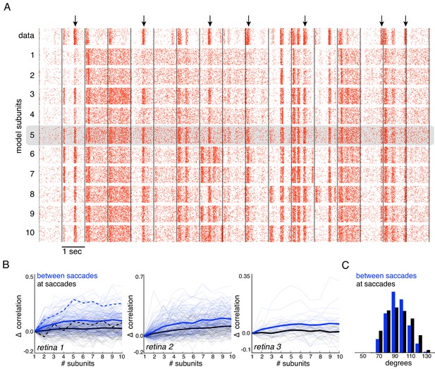
Subunits improve response prediction accuracy for naturalistic stimuli.
(A) Top row: Rasters of responses for an OFF parasol cell from 40 presentations for 30 s long naturalistic stimuli. Natural scene images are presented and spatially jittered, with a new image every 1 s (black lines). Subsequent rows indicate model predictions using different number of subunits (1 to 10), respectively. (B) Change in correlation (relative to the correlation obtained with one subunit) between PSTH for recorded and predicted responses with different number of subunits across three preparations. Individual OFF parasol cells (thin lines) and population average (thick lines) for two conditions: 250 ms immediately following saccades (black) and inter-saccadic stimuli (red). Cell from (A) shown with dashed lines. (C) Distribution of angle between vectors representing the spatial receptive field and natural stimuli (temporally filtered using time course from white noise STA) at saccades (black) and between saccades (blue). Angles with inter-saccadic stimulus are more peaked around 90 degrees, with a standard deviation of 12 degrees, compared with 15 degrees for the saccadic stimulus.
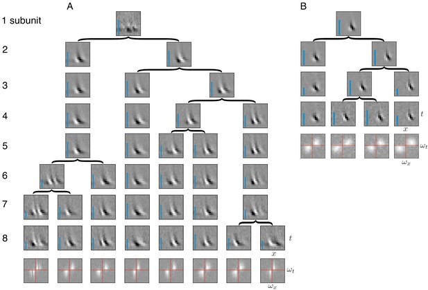
Application of subunit model to V1.
(A) Hierarchical relationship between subunits estimated using responses to flickering bar stimuli for the complex cell featured in Rust et al. (2005). Rows show estimated spatio-temporal filters for different number of subunits (N). As N increases, each successive set of subunits may be (approximately) described as resulting from splitting one subunit into two (indicated by arrows, see Materials and methods). Largest N represents the optimal number of subunits, determined by cross-validation. Fourier magnitude spectrum of the optimal subunits (bottom row) show translational invariance of estimated subunits. Inset : Relative contribution to cell's firing rate for each subunit indicated by height of blue bar (see Equation 6 in Materials and methods). (B) Same as (A) for the simple cell from Rust et al. (2005).
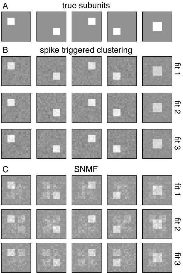
Comparison with spike-triggered non-negative matrix factorization.
(A) Spatial filters for five simulated subunits. Responses are generated by linearly projecting white noise stimulus onto these spatial filters, followed by exponential subunit nonlinearity, summation across subunits and saturating output nonlinearity. (B) Results from the core spike triggered clustering method (without regularization), applied with N = 5 subunits. Rows indicate fits with different initializations. (C) Results from spike-triggered non-negative matrix factorization (SNMF) applied to simulated data. Code provided by Liu et al. (2017). For comparison with to the present method, SNMF applied with no regularization, N = 5 subunits and one perturbation. Similar to (B), rows correspond to fits with different initializations.
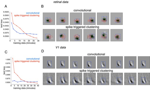
Comparison with convolutional subunit model.
Subunits estimated for the retinal ganglion cell from Figure 1A using a convolutional model, similar to Vintch et al. (2015). The visual stimulus is convolved with a 4 × 4 spatial filter, separately scaled for each location of filter, followed by exponentiation and weighted summation, resulting in Poisson firing rate. Parameters fit using gradient descent. (A) Comparison of neural response predictions for convolutional and spike-triggered clustering analysis. Negative log-likelihood loss on 3 min of test data (y-axis) is shown as a function of increasing duration of training data (x-axis), for the convolutional model (blue) and spike triggered clustering (with locally normalized L1 regularization,=0.1, no output nonlinearity, red). The convolutional model is more efficient (better performance with less training data), but spike triggered clustering performs better with more training data. (B) Estimated subunits for convolutional model (top row) and spike triggered clustering (bottom row, six subunits after cross-validation) for 24 min of training data. Six filters are presented for the convolutional model, translated at location of six strongest learned weights. Columns indicate overlapping subunits from the two methods, matched greedily based on the inner product of the spatio-temporal filters. (C) Similar to (A) for the complex cell from Figure 8A, evaluated on 5 min of test data (y-axis) with a convolutional model that has 8 × 8 spatio-temporal filter (same dimensions as Vintch et al., 2015 and the spike triggered clustering model without regularization. (D) Matched subunits (similar to B) for convolutional model and spike triggered clustering (eight filters selected after cross-validation, see Figure 8A), estimated using 45 min of training data.
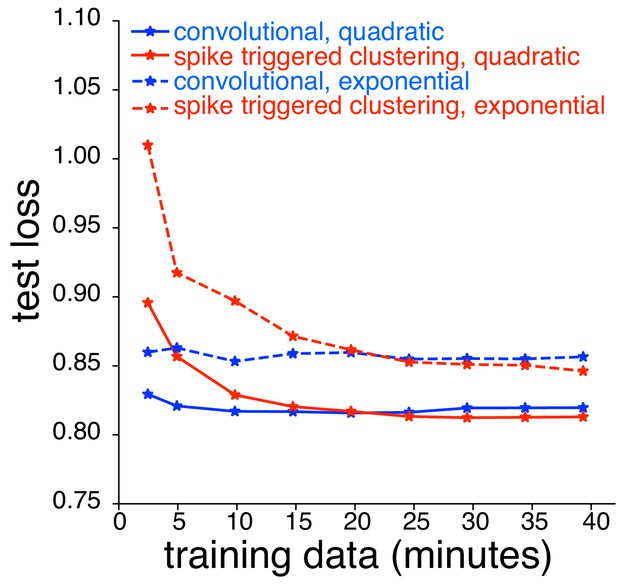
Comparison between spike triggered clustering and convolutional subunit model (Vintch et al., 2015) with quadratic nonlinearity.
Dashed lines correspond to models with exponential nonlinearity (same as Figure 10C); solid lines correspond to quadratic nonlinearity. For the convolutional model, the stimulus is passed through a common subunit filter, with location-specific scales and biases, followed by a quadratic nonlinearity. Parameters are estimated using gradient descent. For spike triggered clustering, the subunit filters are first estimated with spike-triggered clustering (assuming an exponential nonlinearity), and then fine-tuned for the quadratic nonlinearity using gradient descent.
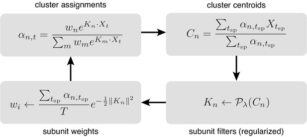
Iterative fitting of subunits, partitioned into four steps.
The subunit kernels () and weights () are randomly initialized, and used to compute soft cluster assignments ( upper left), followed by cluster centroid computation ( - upper right), estimation of subunit kernels ( - lower right) and subunit weights ( - lower left). The summations are only over times when the cell generated a spike ().
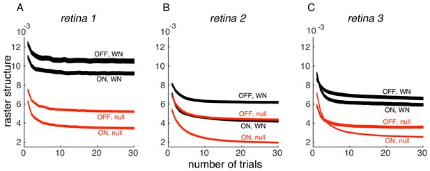
Convergence of PSTH variance.
(A) PSTH variance (y-axis), averaged over ON and OFF populations for white noise (black) and null stimulus (red) as a function of the number of randomly sampled trials (x-axis). Line thickness corresponds to +/- 1 s.d. in estimation error. Same retina as in Figure 5, main paper. (B, C) Same as A, for two other retinas.
Tables
| Reagent type (species) or resource | Designation | Source or reference | Identifiers | Additional information |
|---|---|---|---|---|
| Biological Sample | Macaque retina | UC Davis Primate Research Center | ||
| Biological Sample | Macaque retina | Stanford University | ||
| Biological Sample | Macaque retina | University of California Berkeley | ||
| Biological Sample | Macaque retina | Salk Institue | ||
| Biological Sample | Macaque retina | The Scripps Research Institute | ||
| Chemical compound, drug | Ames' medium | Sigma-Aldrich | Cat #1420 | |
| Software, algorithm | MGL | Gardner Lab | http://gru.stanford.edu/doku.php/mgl/overview | |
| Software, algorithm | MATLAB | Mathworks | ||
| Software, algorithm | Python | https://www.python.org/ | ||
| Software, algorithm | Intaglio | Purgatory Design | ||
| Software, algorithm | Custom spike sorting software | Chichilnisky Lab |


