Combining genomics and epidemiology to analyse bi-directional transmission of Mycobacterium bovis in a multi-host system
- University College Dublin, Ireland
- Animal & Plant Health Agency (APHA), United Kingdom
- University of Edinburgh, United Kingdom
- European Molecular Biology Laboratory, European Bioinformatics Institute (EMBL-EBI), United Kingdom
- University of Glasgow, United Kingdom
- Agri-Food & Biosciences Institute Northern Ireland (AFBNI), United Kingdom
- University of Aberystwyth, United Kingdom
- Genomics Medicine Ireland, Ireland
- Quadram Institute Bioscience, United Kingdom
- University of Oxford, United Kingdom
Figures
Figure 1 with 1 supplement
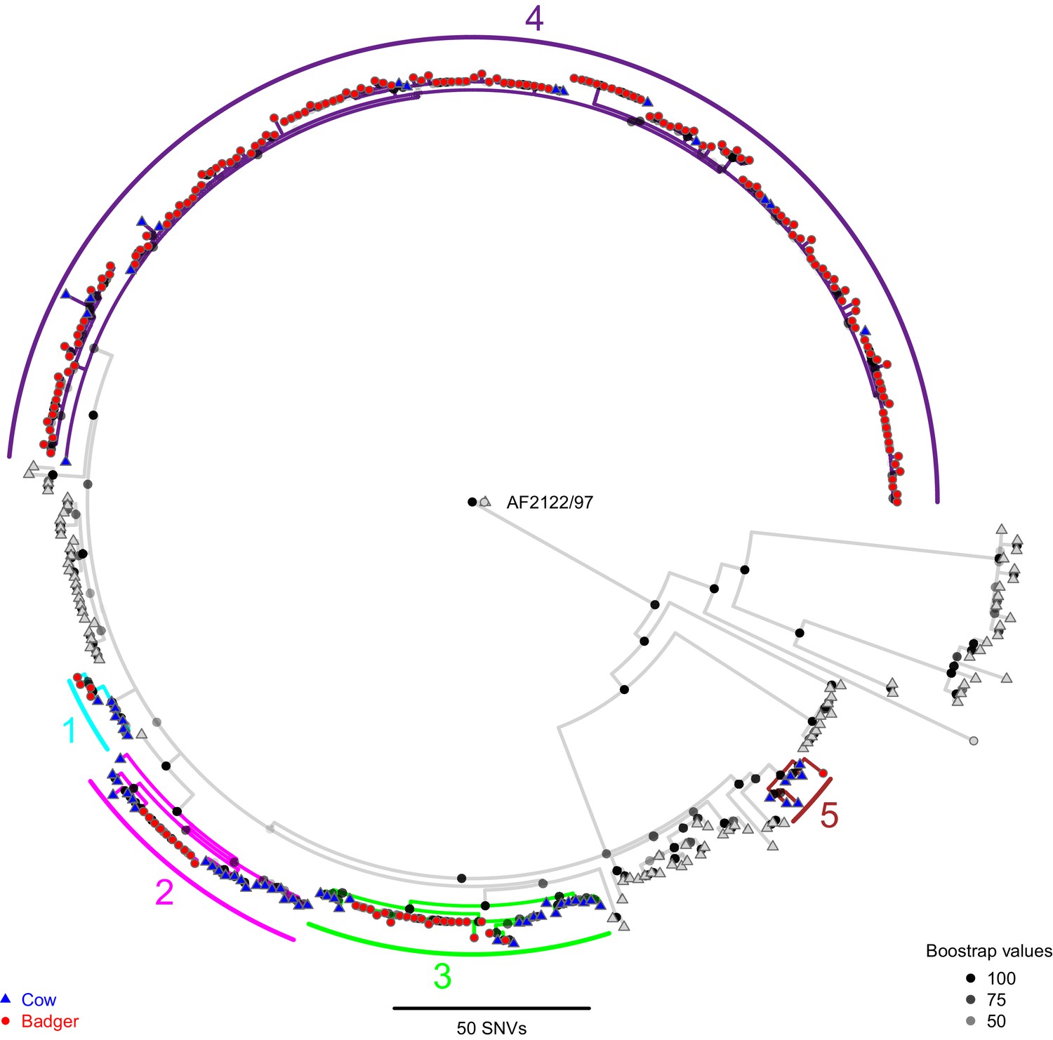
A Maximum Likelihood phylogenetic tree constructed using RAxML (v8.2.11; Stamatakis, 2014) and rooted against the Mycobacterium bovis reference sequence, AF2122/97 (Malone et al., 2017).
Badger and cattle isolates are represented at the tips of the phylogeny by circles and triangles, respectively. Five clades, labelled 1–5, are highlighted with cyan, pink, green, purple, and brown branches, respectively. Cattle and badger isolates within the clades can be distinguished by their shape and colour. Each internal node in the phylogeny is shown as a grey to black shaded circle, with the intensity of the shading indicating the amount of support each node had across 100 bootstraps.
Figure 1—figure supplement 1
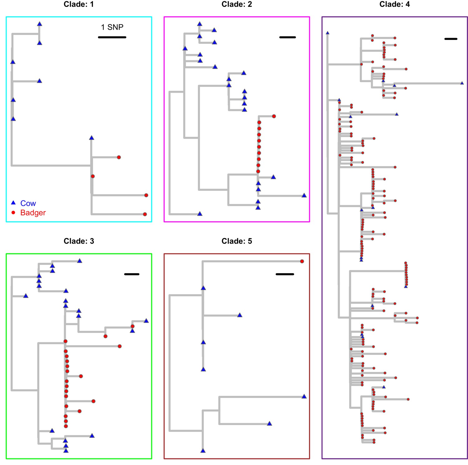
Each of the clades from Figure 1 in the main manuscript are plotted separately.
These clades were extracted from the Maximum Likelihood phylogenetic tree constructed using RAxML (v8.2.11; Stamatakis, 2014) and rooted against the M. bovis reference sequence, AF2122/97 (Malone et al., 2017). Badger and cattle isolates are represented at the tips of the phylogeny by red circles and blue triangles, respectively.
Figure 2 with 4 supplements
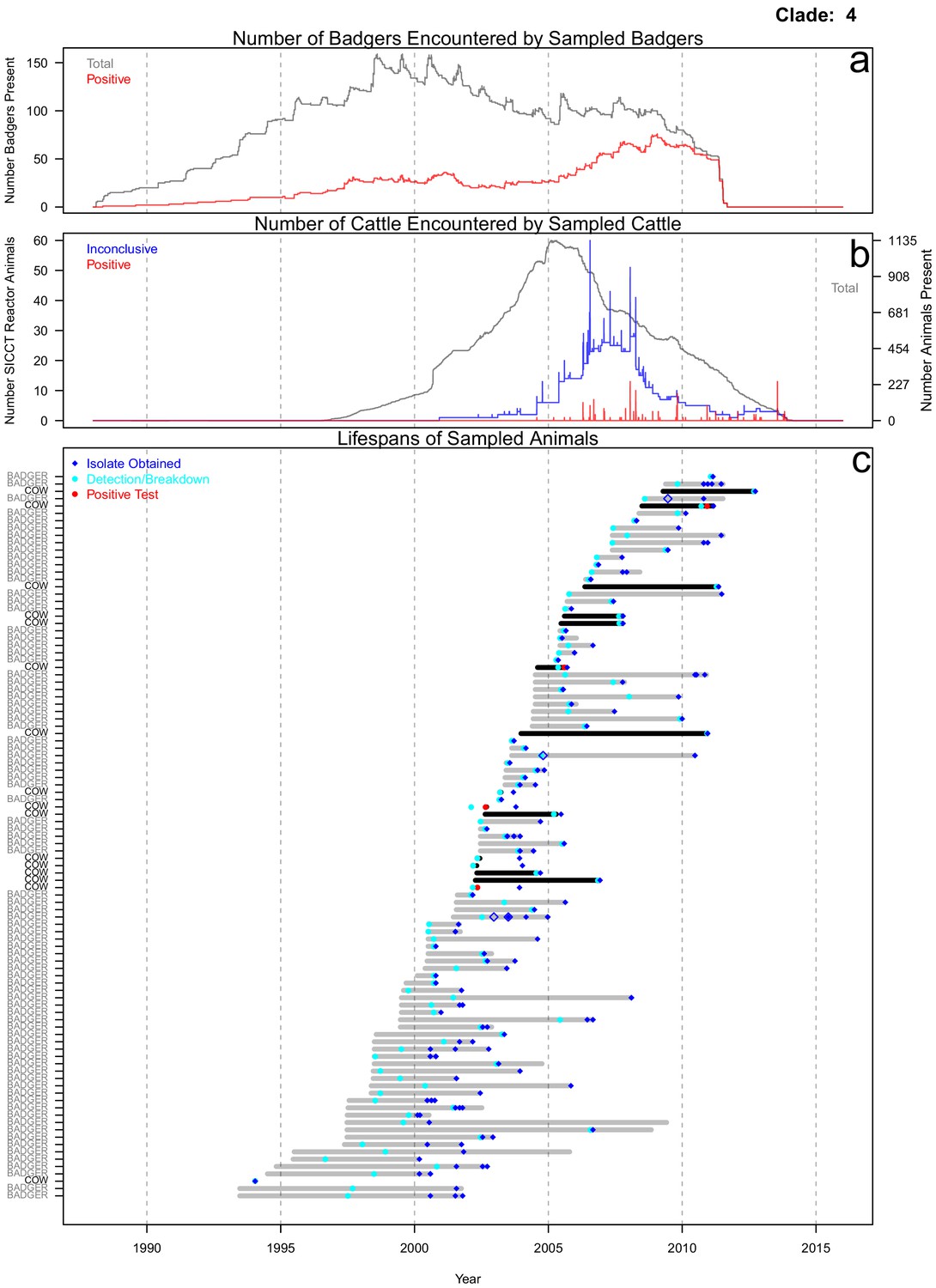
Life history summaries of the sampled and in-contact cattle and badgers associated with clade 4 in Figure 1.
(a) The number of in-contact badgers associated with the sampled badgers (total in grey, number of animals that have tested positive in red). (b) The number of in-contact cattle associated with the sampled cattle (total in grey [right axis], number of animals that reacted inconclusively [red] or positively [blue] to routine skin test [left axis]). In-contact animals are those that lived in the same herd (cattle) or social group (badgers) at the same time as the sampled animals. (c) The recorded lifespans of the sampled cattle (black horizontal bars) and badgers (grey horizontal bars) associated with clade 4.
Figure 2—figure supplement 1
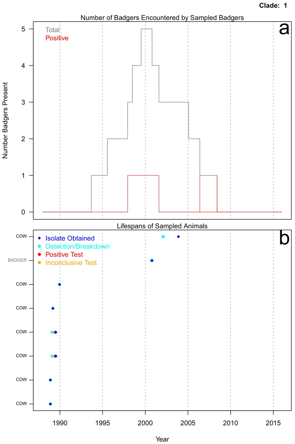
Life history summaries of the sampled and in-contact cattle and badgers associated with clade 1 in Figure 1.
(a) The number of in-contact badgers associated with the sampled badgers (total in grey, number of animals that have tested positive in red). (b) The recorded lifespans of the sampled cattle (black horizontal bars) and badgers (grey horizontal bars) associated with clade 1.
Figure 2—figure supplement 2
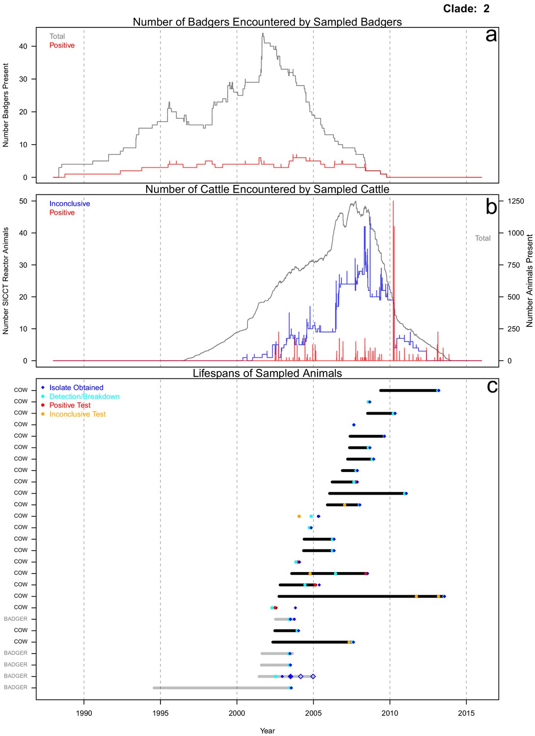
Life history summaries of the sampled and in-contact cattle and badgers associated with clade 2 in Figure 1.
(a) The number of in-contact badgers associated with the sampled badgers (total in grey, number of animals that have tested positive in red). (b) The number of in-contact cattle associated with the sampled cattle (total in grey (right axis), number of animals that reacted inconclusively (red) or positively (blue) to routine skin test (left axis). In-contact animals are those that lived in the same herd (cattle) or social group (badgers) at the same time as the sampled animals. (c) The recorded lifespans of the sampled cattle (black horizontal bars) and badgers (grey horizontal bars) associated with clade 2.
Figure 2—figure supplement 3
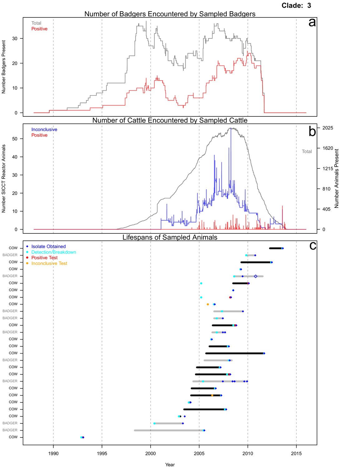
Life history summaries of the sampled and in-contact cattle and badgers associated with clade 3 in Figure 1.
(a) The number of in-contact badgers associated with the sampled badgers (total in grey, number of animals that have tested positive in red). (b) The number of in-contact cattle associated with the sampled cattle (total in grey (right axis), number of animals that reacted inconclusively (red) or positively (blue) to routine skin test (left axis). In-contact animals are those that lived in the same herd (cattle) or social group (badgers) at the same time as the sampled animals. (c) The recorded lifespans of the sampled cattle (black horizontal bars) and badgers (grey horizontal bars) associated with clade 3.
Figure 2—figure supplement 4
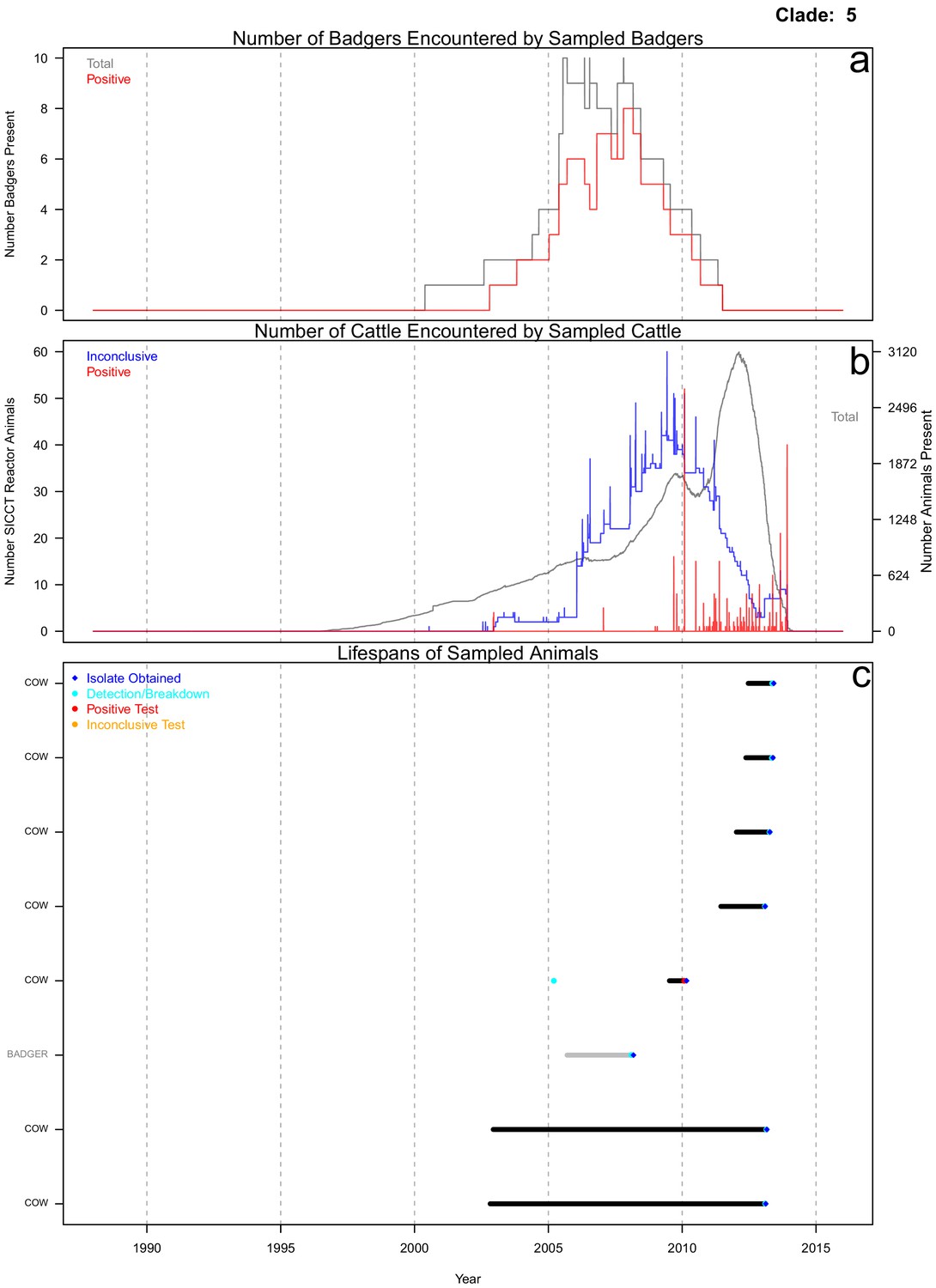
Life history summaries of the sampled and in-contact cattle and badgers associated with clade 5 in Figure 1.
(a) The number of in-contact badgers associated with the sampled badgers (total in grey, number of animals that have tested positive in red). (b) The number of in-contact cattle associated with the sampled cattle (total in grey (right axis), number of animals that reacted inconclusively (red) or positively (blue) to routine skin test (left axis). In-contact animals are those that lived in the same herd (cattle) or social group (badgers) at the same time as the sampled animals. (c) The recorded lifespans of the sampled cattle (black horizontal bars) and badgers (grey horizontal bars) associated with clade 5.
Figure 3 with 1 supplement

Comparison of likelihood scores and inter-species transition rate estimates from the BASTA analyses.
Model structure is described in Figure 6, and for each model the sizes of defined demes were held equal or allowed to vary. (a) The Akaike Information Criterion Markov Chain Monte Carlo (AICM; Baele et al., 2013) scores (lower is better) calculated for each of the representations of a structured population analysed in BASTA (Figure 6). The vertical lines show the lower and upper (2.5% and 97.5%, respectively) bounds of the AICM scores computed on 100 bootstrapped posterior likelihoods. (b) Estimated inter-species transition rates for each model. Where multiple badgers-to-cattle and cattle-to-badgers transition rates were estimated (see Figure 6), the values were summed. The values above each vertical line represent the posterior probability of each rate, either as a mean of probabilities associated with multiple estimated rates (for the 3Deme_outerIsBadgers, 4Deme, 6Deme, and 8Deme models) or a single probability (for the 2Deme, 3Deme_outerIsBoth, and 3Deme_outerIsCattle models). (c) The number of transitions between the known and estimated states counted on each phylogenetic tree in the posterior distribution produced by the ‘2Deme_equal’ structured population model analysed in BASTA (counting is illustrated in Figure 3—figure supplement 1). The vertical lines show the lower and upper (2.5% and 97.5%, respectively) bounds of the distributions.
Figure 3—figure supplement 1
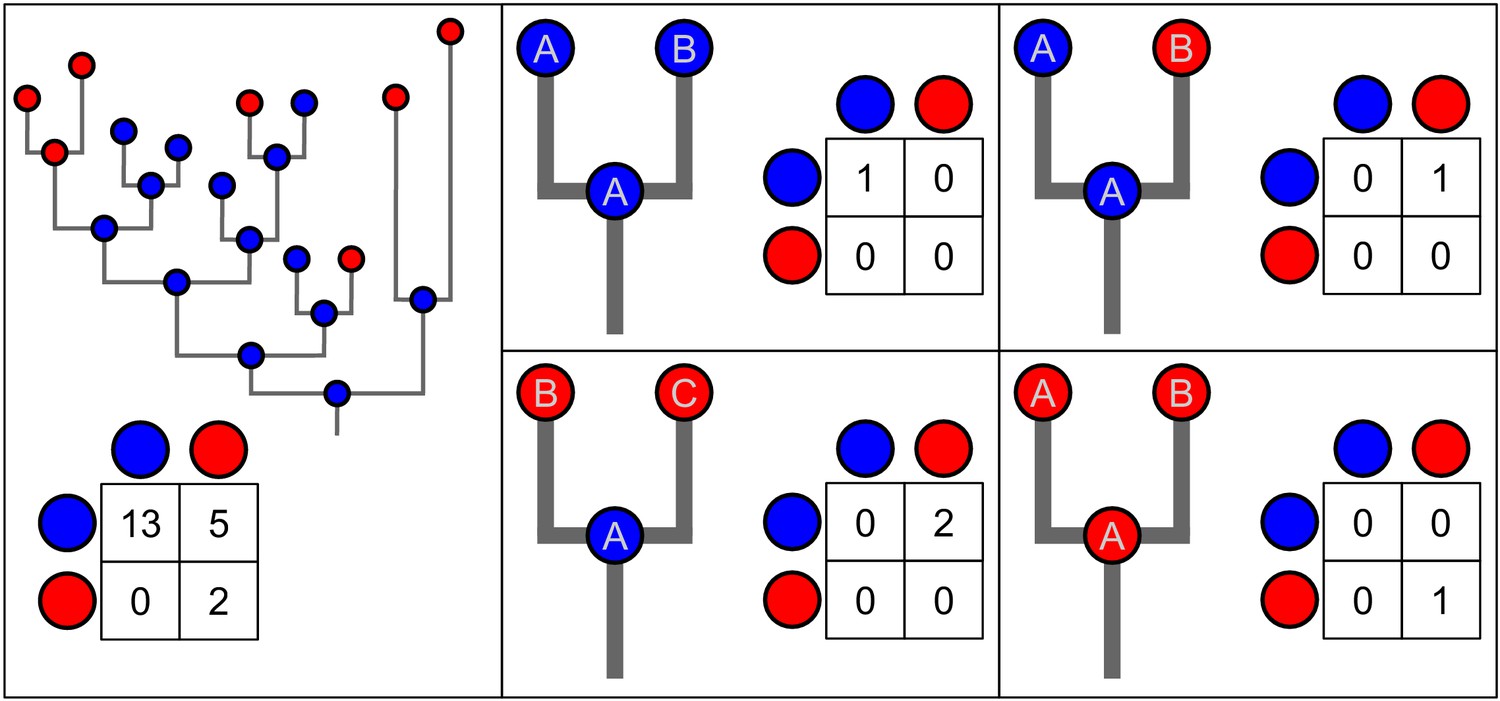
Diagrams illustrating how the transmission events were counted on each of the phylogenies in the posterior distributions produced by BASTA.
These counts are shown in panel c ofFigure 3. Each diagram has a simple phylogeny with the estimated states (blue or red) of a parent and its two daughter nodes. The count of the number of transition events on each phylogeny is recorded in a matrix. Transitions are counted in the direction from parent to daughter. Each node has an ID to illustrate the situations when the parent node is assumed to represent one of its daughter nodes earlier in evolutionary time.
Figure 4
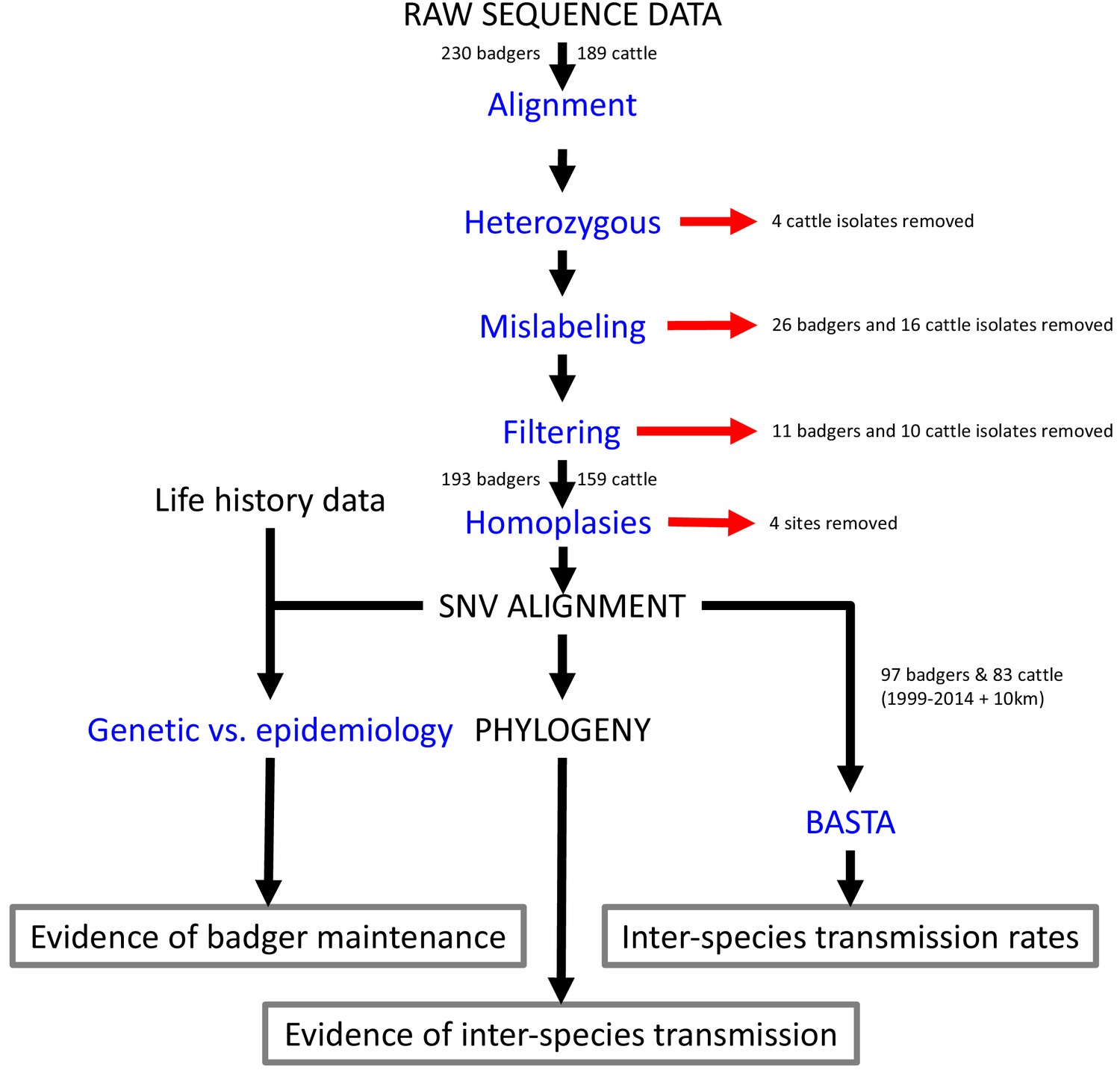
Steps involved in the analysis of M.bovis whole genome sequences and epidemiological data.
Analyses are shown in blue and outputs and inputs in black. Red arrows represent the removal of data. The three main outputs are highlighted with grey boxes. SNV: Single Nucleotide Variant. BASTA: Bayesian Structured coalescent Approximation.
Figure 5
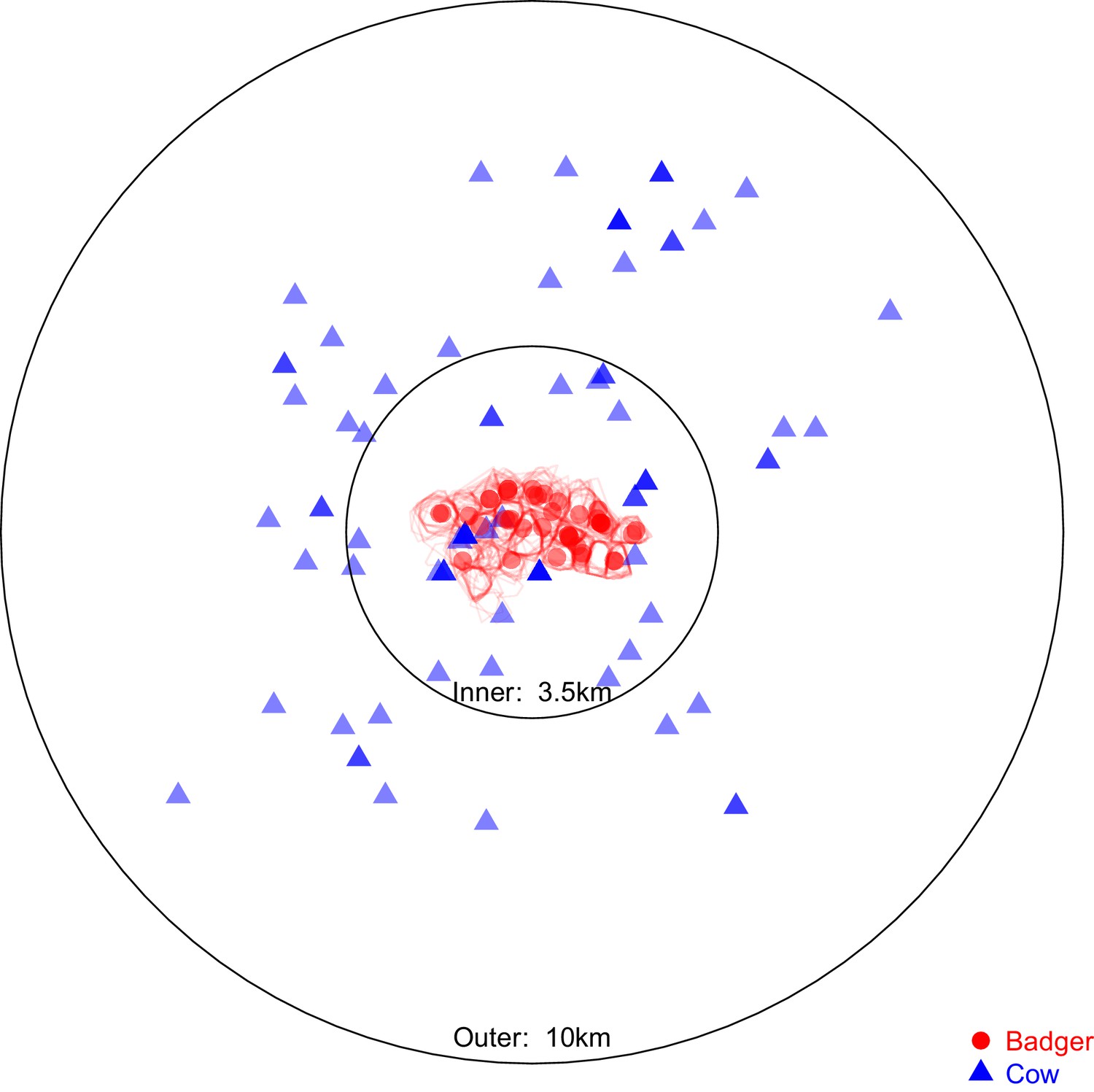
Sampling locations of the 97 badgers and 83 cattle associated with the Mycobacterium bovis sequences selected for analysis in BEAST2.
Location represents the registered address of each sampled farm or the centroid of the estimated sampled badger social group’s territory boundary (indicated by the red polygons). The overlaid circles were used to split the cattle- and badger-derived M. bovis sequences into ‘inner’ and ‘outer’ populations, the distances refer to the radius of each circle. The ‘inner’ circle was defined such that it contained all the locations associated with the available badger-derived and closest (within the badger’s recorded home range of <1 km2 [Gittleman and Harvey, 1982; Garnett et al., 2005; Macdonald et al., 2008; Roper et al., 2003]) surrounding cattle-derived M. bovis sequences.
Figure 6

Deme assignment diagrams illustrating the different demes (sub-populations) defined in a range of structured population analyses conducted using BASTA.
In each analysis, the Mycobacterium bovis sequences available were assigned to each deme based upon the sampled species and their sampling location. The grey doughnut in the badger demes represents an un-sampled population. These diagrams are based on the spatial associations of the badger and cattle-derived M. bovis sequences shown in Figure 5.
Appendix 1—figure 1
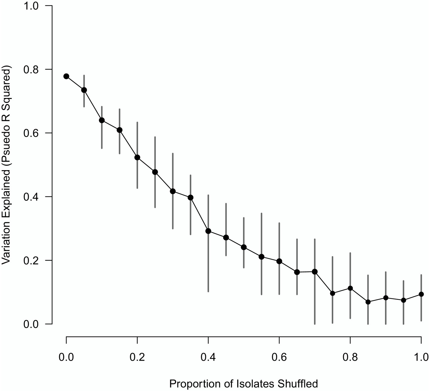
The impact of shuffling varying proportions of the M. bovis isolate sequences on the variation explained by the Random Forest model.
The mean of 10 replicates is shown as a black point, with vertical lines representing the min and max values.
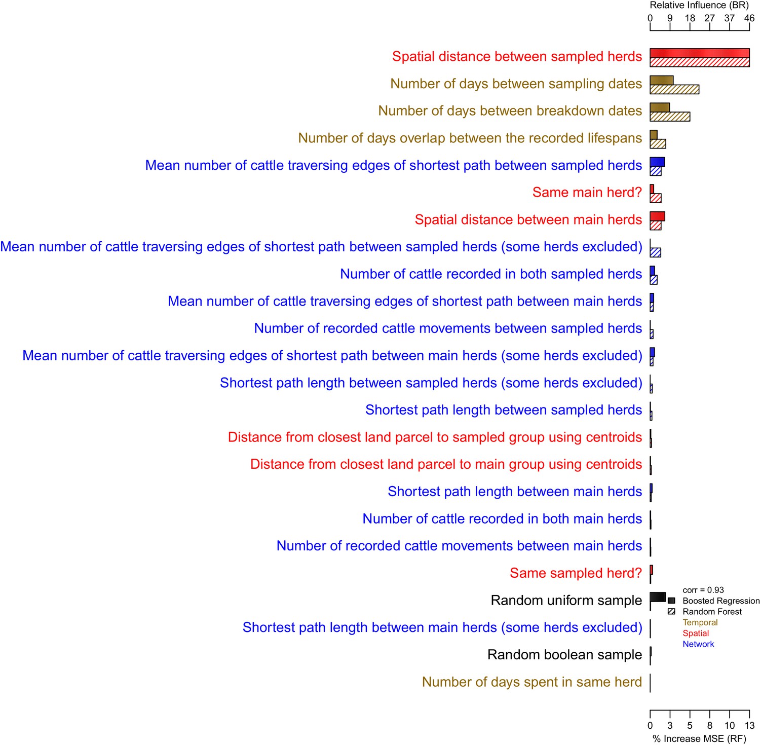
Appendix 1—figure 2
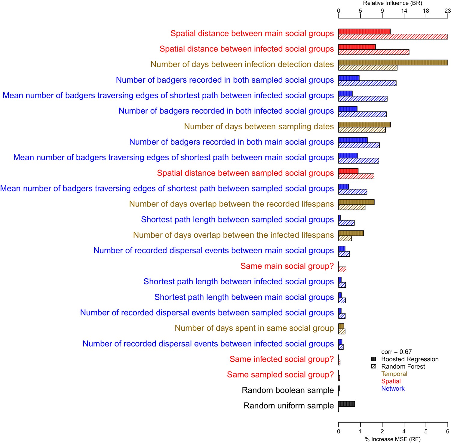
The importance of each epidemiological metric in explaining variation in the inter-badger-sequence genetic distance distribution.
Metrics are coloured according to whether they used temporal (gold), spatial (red), or network (blue) information. The correlation (Pearson’s correlation) of the variable importance from the Random Forest and Boosted Regression models is reported in the legend. Two random metrics were included, a sample from a uniform distribution and a sample from a Boolean distribution, in the regression models.
Appendix 1—figure 3
The importance of each epidemiological metric in explaining variation in the inter-cattle-sequence genetic distance distribution.
Metrics are coloured according to whether they used temporal (gold), spatial (red), or network (blue) information. The correlation (Pearson’s correlation) of the variable importance from the Random Forest and Boosted Regression models is reported in the legend. Two random metrics were included, a sample from a uniform distribution and a sample from a Boolean distribution, in the regression models.
Appendix 1—figure 4
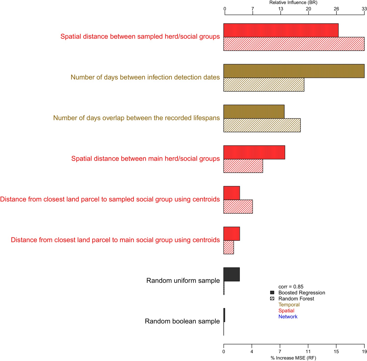
The importance of each epidemiological metric in explaining variation in the badger-cattle-sequence genetic distance distribution.
Metrics are coloured according to whether they used temporal (gold), or spatial (red), or network (blue) information. The correlation (Pearson’s correlation) of the variable importance from the Random Forest and Boosted Regression models is reported in the legend. Two random metrics were included, a sample from a uniform distribution and a sample from a Boolean distribution, in the regression models.
Appendix 1—figure 5
Partial dependence plots estimating the average marginal effect of each epidemiological metric fitted in the Random Forest regression models on the inter-badger-sequence genetic distance distribution.
The Y axis in each sub-plot represents the genetic distance distribution of the number of the differences between the M. bovis genomes. The X axis of each plot corresponds to the range associated with the corresponding epidemiological metrics. The red line represents the average marginal effect on the predicted genetic distance for each value of the epidemiological metric. Metrics with low importance in the Random Forest models were removed (% Mean Squared Error change of < 0.5%).
Appendix 1—figure 6
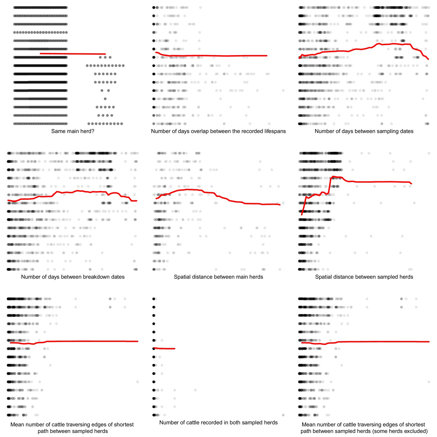
Partial dependence plots estimating the average marginal effect of each epidemiological metric fitted in the Random Forest regression models on the inter-cattle-sequence genetic distance distribution.
The Y axis in each sub-plot represents the genetic distance distribution of the number of the differences between the M. bovis genomes. The X axis of each plot corresponds to the range associated with the corresponding epidemiological metrics. The red line represents the average marginal effect on the predicted genetic distance for each value of the epidemiological metric. Metrics with low importance in the Random Forest models were removed (% Mean Squared Error change of < 0.5%).
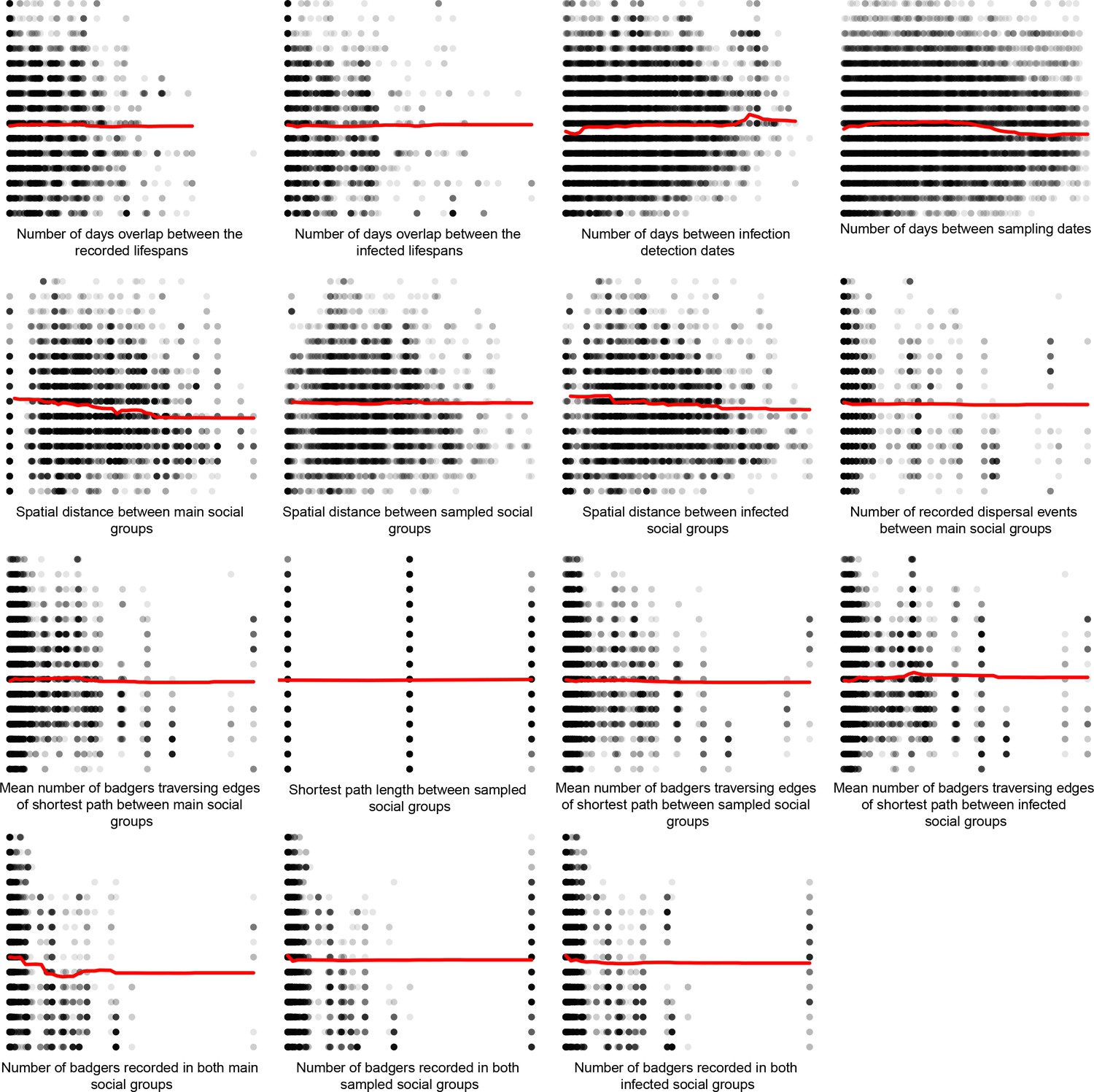
Appendix 1—figure 7
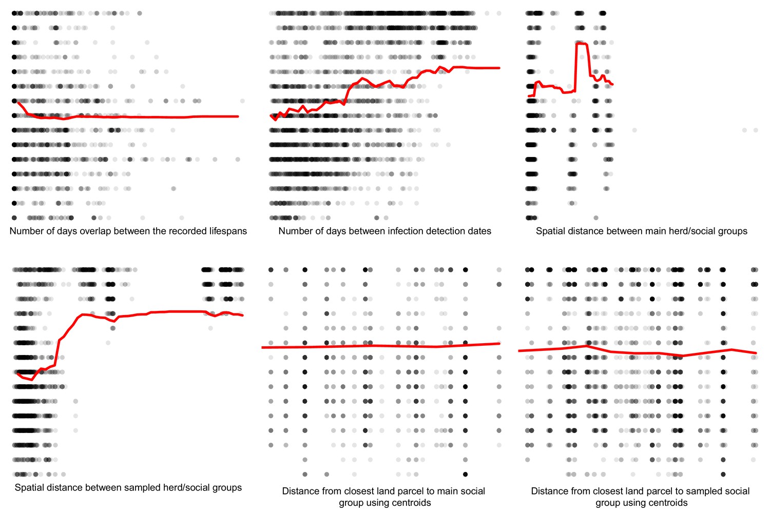
Partial dependence plots estimating the marginal effect of each epidemiological metric fitted in the Random Forest regression models on the badger-cattle-sequence genetic distance distribution.
The Y axis in each sub-plot represents the genetic distance distribution of the number of the differences between the M. bovis genomes. The X axis of each plot corresponds to the range associated with the corresponding epidemiological metrics. The red line represents the average marginal effect on the predicted genetic distance for each value of the epidemiological metric. Metrics with low importance in the Random Forest models were removed (% Mean Squared Error change of < 0.5%).
Appendix 2—figure 1
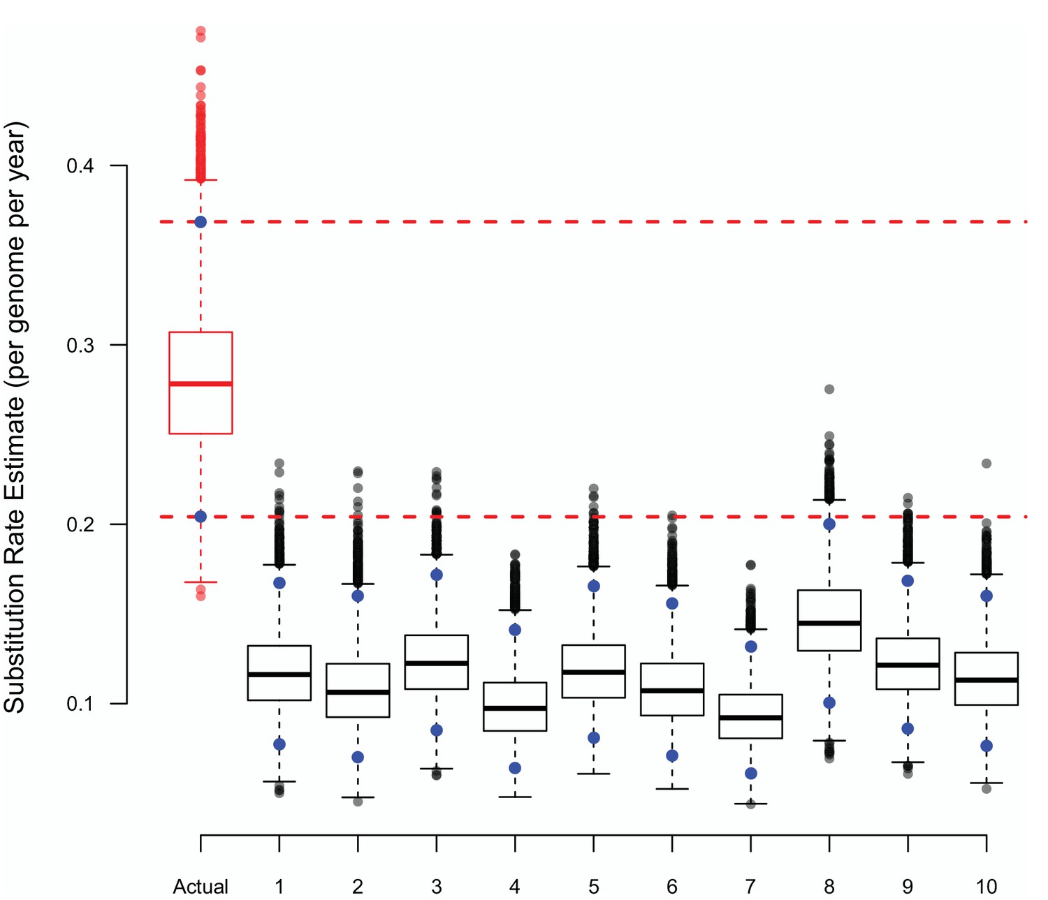
The substitution rate estimates from BASTA using either true or randomly shuffled sampling dates.
The upper (97.5%) and lower (2.5%) bounds of each distribution are shown as blue points, the horizontal dashed lines represent the same bounds for the estimates based on the actual dates. Each BASTA analysis using a two population (badgers and cattle) structure, allowed different but constant population sizes, and relaxed clock model based upon an HKY substitution model.
Tables
Appendix 1—table 1
Epidemiological metrics capturing the spatial, temporal, and network relationships between a pair of sampled animals.
Whether or not the metric was used in the badger–badger, cattle–cattle, and badger–cattle comparisons is indicated.
| Epidemiological metrics | Badger-Badger | Cattle-Cattle | Badger-Cattle |
|---|---|---|---|
| Same main [herd/social group]? | YES | YES | NO |
| Same sampled [herd/social group]? | YES | YES | NO |
| Same infected [herd/social group]? | YES | NO | NO |
| Spatial distance between main [herd/social group]s | YES | YES | YES |
| Spatial distance between sampled [herd/social group]s | YES | YES | YES |
| Spatial distance between infected [herd/social group]s | YES | NO | NO |
| Distance from closest land parcel to main [herd/social group] using centroids | NO | NO | YES |
| Distance from closest land parcel to sampled [herd/social group] using centroids | NO | NO | YES |
| Number of days overlap between the recorded lifespans | YES | YES | YES |
| Number of days overlap between the infected lifespans | YES | NO | NO |
| Number of days spent in same [herd/social group] | YES | YES | NO |
| Number of days between infection detection dates | YES | NO | YES |
| Number of days between sampling dates | YES | YES | NO |
| Number of days between breakdown dates | NO | YES | NO |
| Number of recorded [cattle movements/dispersal events] between main [herd/social group]s | YES | YES | NO |
| Number of recorded [cattle movements/dispersal events] between sampled [herd/social group]s | YES | YES | NO |
| Number of recorded [cattle movements/dispersal events] between infected [herd/social group]s | YES | NO | NO |
| Shortest path length between main [herd/social group]s | YES | YES | NO |
| Mean number of [cattle/badgers] traversing edges of shortest path between main [herd/social group]s | YES | YES | NO |
| Shortest path length between sampled [herd/social group]s | YES | YES | NO |
| Mean number of [cattle/badgers] traversing edges of shortest path between sampled [herd/social group]s | YES | YES | NO |
| Shortest path length between infected [herd/social group]s | YES | NO | NO |
| Mean number of [cattle/badgers] traversing edges of shortest path between infected [herd/social group]s | YES | NO | NO |
| Number of [cattle/badgers] recorded in both main [herd/social group]s | YES | YES | NO |
| Number of [cattle/badgers] recorded in both sampled [herd/social group]s | YES | YES | NO |
| Number of [cattle/badgers] recorded in both infected [herd/social group]s | YES | NO | NO |
| Shortest path length between main [herd/social group]s (some [herd/social group]s excluded) | NO | YES | NO |
| Mean number of [cattle/badgers] traversing edges of shortest path between main [herd/social group]s (some [herd/social group]s excluded) | NO | YES | NO |
| Shortest path length between sampled [herd/social group]s (some [herd/social group]s excluded) | NO | YES | NO |
| Mean number of [cattle/badgers] traversing edges of shortest path between sampled [herd/social group]s (some [herd/social group]s excluded) | NO | YES | NO |
| Shortest path length between infected [herd/social group]s (some [herd/social group]s excluded) | NO | YES | NO |
| Mean number of [cattle/badgers] traversing edges of shortest path between main [herd/social group]s (some [herd/social group]s excluded) | NO | YES | NO |
Appendix 1—table 2
The 15 M. bovis isolates whose inter-isolate genetic distances were poorly predicted (median difference between actual and predicted genetic distances outside 95% percentile) by the Random Forest and/or Boosted Regression models.
Those isolates whose spoligotypes did not match the phylogenetic patterns are also listed.
| Isolate ID | Outlier - Random Forest | Outlier - Boosted Regression | Phylogenetic-Spoligotype mismatch |
|---|---|---|---|
| WB65 | YES | YES | NO |
| WB15 | YES | YES | NO |
| WB137 | NO | YES | NO |
| WB70 | YES | YES | NO |
| WB98 | YES | YES | NO |
| WB99 | YES | YES | NO |
| WB71 | NO | YES | YES |
| WB105 | YES | YES | YES |
| WB106 | YES | YES | NO |
| WB74 | YES | YES | NO |
| WB75 | YES | YES | NO |
| WB107 | NO | NO | YES |
| WB72 | NO | NO | YES |
| WB96 | YES | NO | NO |
| WB100 | YES | NO | YES |
Author response table 1
| 2 demes | 3 demes – outer is both | 3 demes – outer is cattle | 3 demes – outer is badgers | 4 demes | 6 demes – north and south | 6 demes – east and west | 8 demes – north and south | 8 demes – east and west | |
|---|---|---|---|---|---|---|---|---|---|
| CB | 1 | 1 | 1 | 2 | 2 | 3 | 3 | 4 | 4 |
| BC | 1 | 1 | 1 | 2 | 2 | 3 | 3 | 4 | 4 |
Additional files
Download links
A two-part list of links to download the article, or parts of the article, in various formats.
Downloads (link to download the article as PDF)
Open citations (links to open the citations from this article in various online reference manager services)
Cite this article (links to download the citations from this article in formats compatible with various reference manager tools)
Combining genomics and epidemiology to analyse bi-directional transmission of Mycobacterium bovis in a multi-host system
eLife 8:e45833.
https://doi.org/10.7554/eLife.45833


