A quantitative model of conserved macroscopic dynamics predicts future motor commands
- University of Pennsylvania, United States
Figures
Figure 1 with 2 supplements
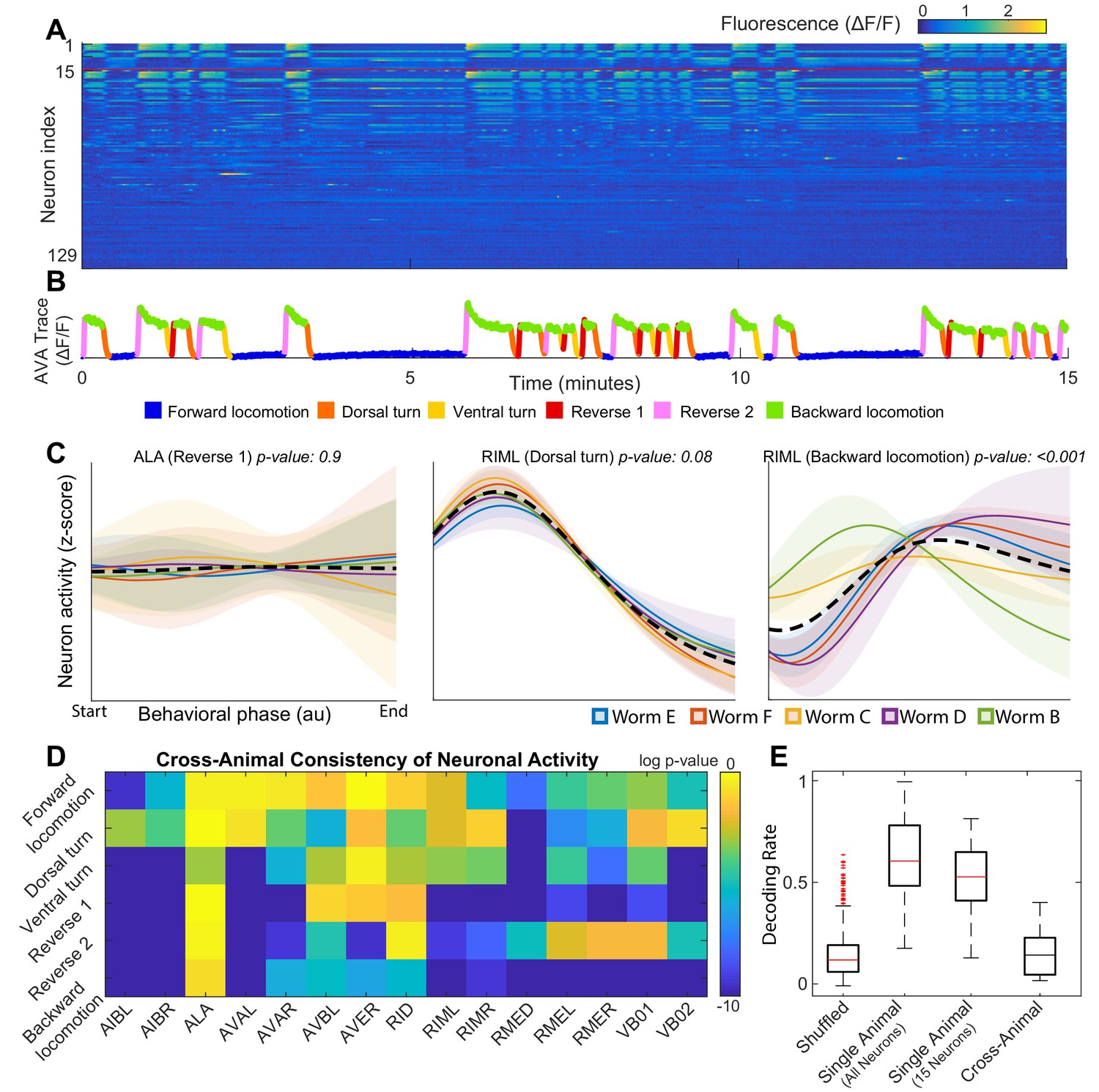
Neuronal activity is consistently different in different individuals.
(A) Calcium signals () recorded in one animal for ∼15 min by Kato et al. (2015). Each row represents a single neuron. The top 15 rows (above the red line) correspond to neurons unambiguously identified in all animals (shared neurons). (B) Trace of the AVA neuron colored by behavioral state as defined by Kato et al. (2015). (C) Neuronal activity of representative neurons plotted as a function of behavioral phase (Materials and methods) in a single behavior grouped by animal. Colored solid lines show mean activity for each animal. Shaded regions show 95% confidence intervals. Mean and confidence intervals are computed across multiple cycles of the same behavior in each animal. The dashed black line shows the mean across all cycles of the behavior in all animals. The cross-animal mean for ALA and RIML (Dorsal turn) is a good approximation of activity in each animal individually. In contrast, the cross-animal mean of RIML (Backward locomotion) does not represent any individual. Thus, activity of RIML is consistently different among individuals during backward locomotion. (D) Probabilities that neuronal activity from different individuals was drawn from the same distribution (Materials and methods) computed for each neuron in each locomotor behavior. Activity of most neurons differs consistently among individuals in at least one locomotor behavior. (E) Attempts to decode the onset of backwards locomotion are successful within each animal individually using either all neurons or the 15 shared neurons. This confirms that neuronal activation is stereotyped in each animal. Yet decoding fails across animals. Probability of decoding onset of backwards locomotion in one animal on the basis of neuronal activity averaged across other four animals is indistinguishable from chance. Thus, averaging neuronal activity across individuals disrupts behaviorally relevant information. Box plots show distribution of decoding rates bootstrapped across animals and bi-partitions of the data into training and validation datasets (Materials and methods).
Figure 1—figure supplement 1
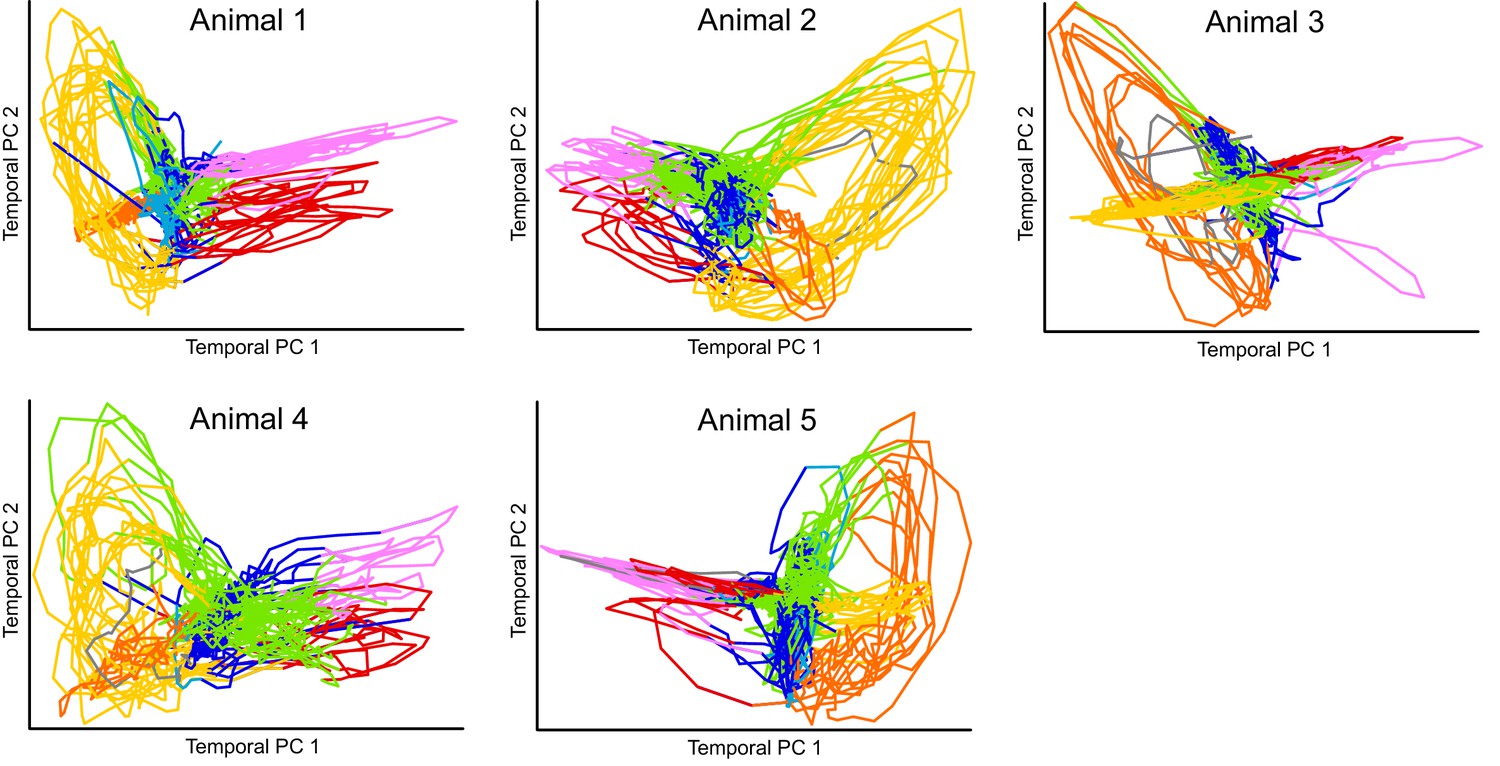
Projection of calcium imaging data onto Temporal PCs.
Time derivative of neuronal activity in each animal is projected onto it’s corresponding first two principal components similar to Kato et al. (2015). The only preprocessing applied to the data was a Gaussian smoothing with sigma of one time step. Colors correspond to the fictive behaviors assigned by Kato et al. (2015). Note that the projection of each individual reveals clear loops in the dynamics of the nervous system. Kato et al. refer to this projection as Temporal PCA. Note that activity from each animal is projected onto its own coordinate system. Also see Figure 1—video 1.
Figure 1—video 1
Projection of calcium imaging data onto shared TPCAs.
The shared set of 15 neurons recorded in each animal is used to construct shared Temporal PCs using the same method as in Kato et al. (2015). The video shows the data from all animals projected onto the first 3 components of the shared Temporal PCA. To produce these PCs the data from Figure 1—figure supplement 1 (without z-scoring) was concatenated together and subjected to PCA. This results in 15000 observations, which, accounting for a mean autocorrelation in the data of 150 time steps yields approximately 100 independent observations. Colors correspond to the fictive behaviors assigned by Kato et al. (2015). The structure apparent in the individual animal Temporal PCA projections has been lost (Figure 1—figure supplement 1).
Figure 2 with 4 supplements
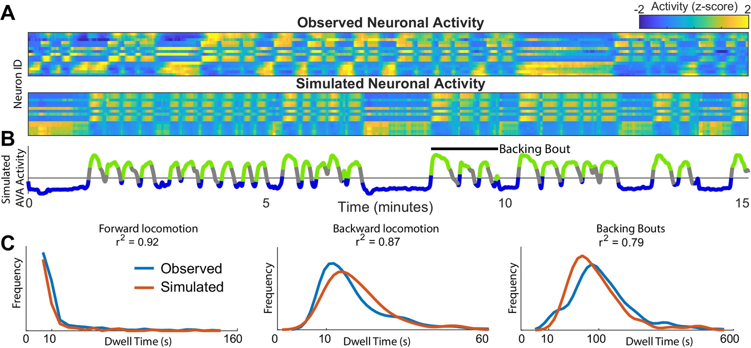
Simulations of the dynamics faithfully reproduce neuronal activity and behavioral statistics.
(A) Experimentally observed (top) and simulated (bottom) activity of 15 shared neurons plotted as in Figure 1A. (B) Trace of the simulated AVA neuron colored according to the inferred behavioral state. In contrast to Figure 1, color here expresses neuronal activity as z-score computed for each neuron individually. Behavioral states are assigned based on experimentally observed distribution of behaviors for each point in phase space (blue forward locomotion; green backward locomotion) (Materials and methods). Both A and B are plotted on the same time-axes. Because of under-sampling, transitions between forward and backward locomotions are left unassigned (gray). (C) Dwell time distributions for forward locomotion, backward locomotion and backing bouts (blue experimentally observed; orange simulated). Backing bouts were defined as repeated episodes of backing behavior separated by short forward locomotion states lasting at most 30 frames ( 10 s) (e.g. black line in B). Although the manifold is constructed on the basis of transition probabilities between states separated by <1 s., the manifold successfully predicts statistics of behaviors over 100 s.
Figure 2—figure supplement 1
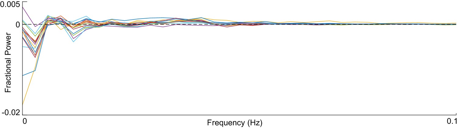
Neuronal activity trace spectral residues.
Each line gives the difference in fractional power of the spectrum of the observed neuron and it’s simulated partner. The simulated and observed spectra are in good agreement for all frequencies above 0.05 Hz (where finite data artifacts are most prevalent).
Figure 2—figure supplement 2
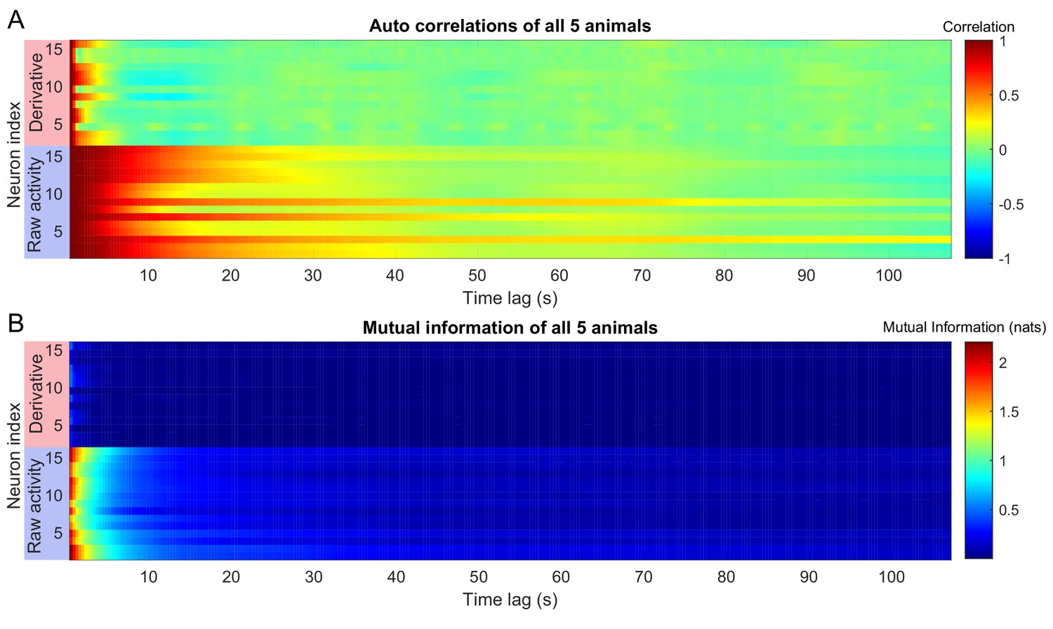
Auto correlations and auto mutual information inform expected delay time scales.
The auto correlation (A) and auto mutual information (B) for the experimentally observed neuronal activation in the (Kato et al., 2015) dataset (blue boxes), along with the auto correlation and auto mutual information of their derivatives (red boxes) is plotted for time lags up to 100 s. In the article, we used autocorrelations to estimate an appropriate choice of . We selected a delay time based on the minimum (across neurons) auto correlation time constant (10 frames, 4 s). Choice of is not trivial for a multivariate system. However, the results do not strongly depend on this choice so long as the total delay time is ∼ 50 frames (∼ 18 s) Figure 2—figure supplement 3.
Figure 2—figure supplement 3

Effect of delay embedding parameters on model accuracy.
The delay embedding parameters (number of delays and delay length) are varied to test for robustness. Dots represent a unique pair of parameters. For each pair the method is rerun on all 15 neurons from all five animals in the Kato et al. (2015) dataset and the accuracy of this new model’s simulated motor command dwell time distributions are compared to the observed distributions. Color represents the relative information compared to the original model. Relative information of 1 means that the model constructed using a particular set of delay lengths and number of delays performed as well as the parameter values used in the manuscript (red diamond) (Materials and methods). Note that as long as the total delay length is about 50 time steps the model tends to perform well (about 60% of the original model’s performance).
Figure 2—figure supplement 4
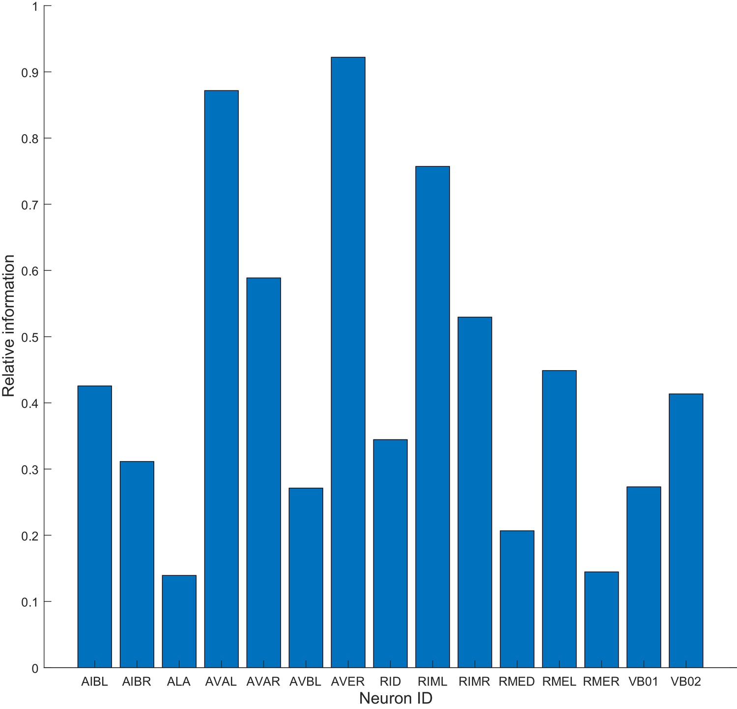
Model can be constructed on the basis of a single neuron.
The method is applied to data from a single neuron and used to build the dwell times of motor commands as in Figure 3. Relative information of 1 means that the model constructed on a single neuron performed the same as the model based on all 15 neurons (Materials and methods). Note that AVAL, AVER and RIML approximate performance obtained when all 15 neurons are used.
Figure 3 with 1 supplement
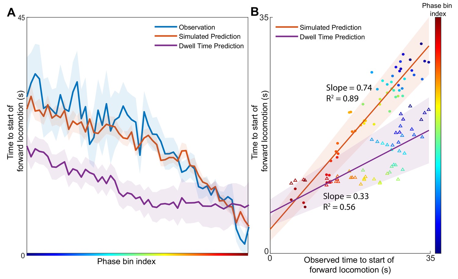
Position in the phase space determines the expected time of future behavioral transitions.
We explore the region of phase space where most instances of motor commands for backward locomotion are terminated and give rise to commands for forward locomotion. (A) The distribution of times to start of forward locomotion (orange line → mean, orange shading → 95% confidence intervals) is simulated as a function of starting phase. Observed distribution of times to start of forward locomotion in 11 new animals from Nichols et al. (blue line → mean, blue shading → 95% confidence intervals) are calculated for each phase bin in the same region. For each phase bin we also computed the average time since onset of backward locomotion. We then used this average time and the dwell time distribution of backward locomotion to calculate the expected time of termination of backward locomotion (purple line → mean, purple shading → 95% confidence intervals) (Materials and methods). This null hypothesis is grossly inaccurate. (B) Times to start of forward locomotion for both the simulation (orange line → mean, orange shading → 95% confidence intervals, filled circles), and the null model built on dwell times (purple line → mean, purple shading → 95% confidence intervals, empty triangles) are plotted against the time to start of forward locomotion command of the newly observed Nichols et al. animals. Individual points show the average time to start of forward locomotion for each individual phase bin (point color). The simulation (orange) is a good predictor of the newly observed data. In contrast, the null model based on dwell times (purple) consistently underestimates the time until initiation of forward locomotion (p < 0.0001).
Figure 3—figure supplement 1
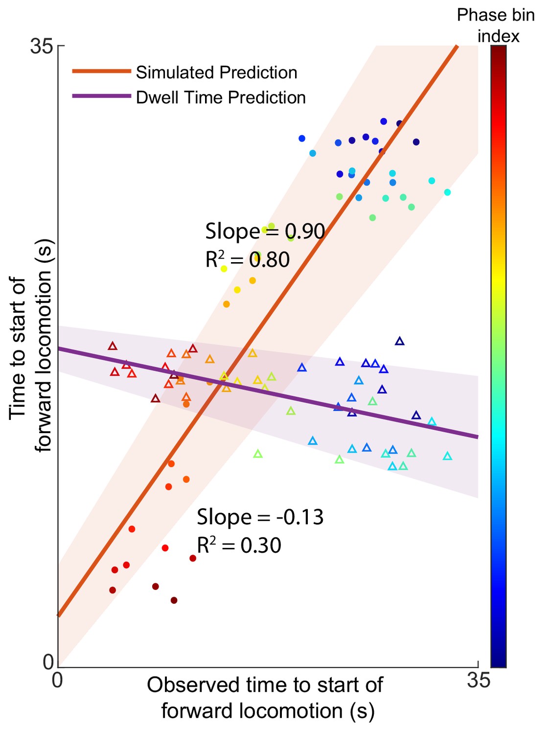
Predictions of expected time to switch of behavior are still valid without AVA.
AVAL and AVAR were removed from the five animals in the Kato et al dataset and the Nichols et al dataset used for model validation. The prediction of the expected time to motor command transition was performed as described in the article. The removal of AVA does not dramatically effect the results of the model. Times to start of forward locomotion command for both the simulation (orange line → mean, orange shading → 95% confidence intervals, filled circles), and the null model built on dwell times (purple line → mean, purple shading → 95% confidence intervals, empty triangles) are plotted against the time to start of forward locomotion command of the newly observed Nichols et al. animals. Individual points show the average time to start of forward locomotion for each individual phase bin (point color). Note that the relative information as defined in Figure 2—figure supplement 4 and Figure 2—figure supplement 3 is 0.91 for the model without AVA (Materials and methods). This means that losing information from AVA only reduces the model’s performance by ∼10%.
Figure 4 with 3 supplements
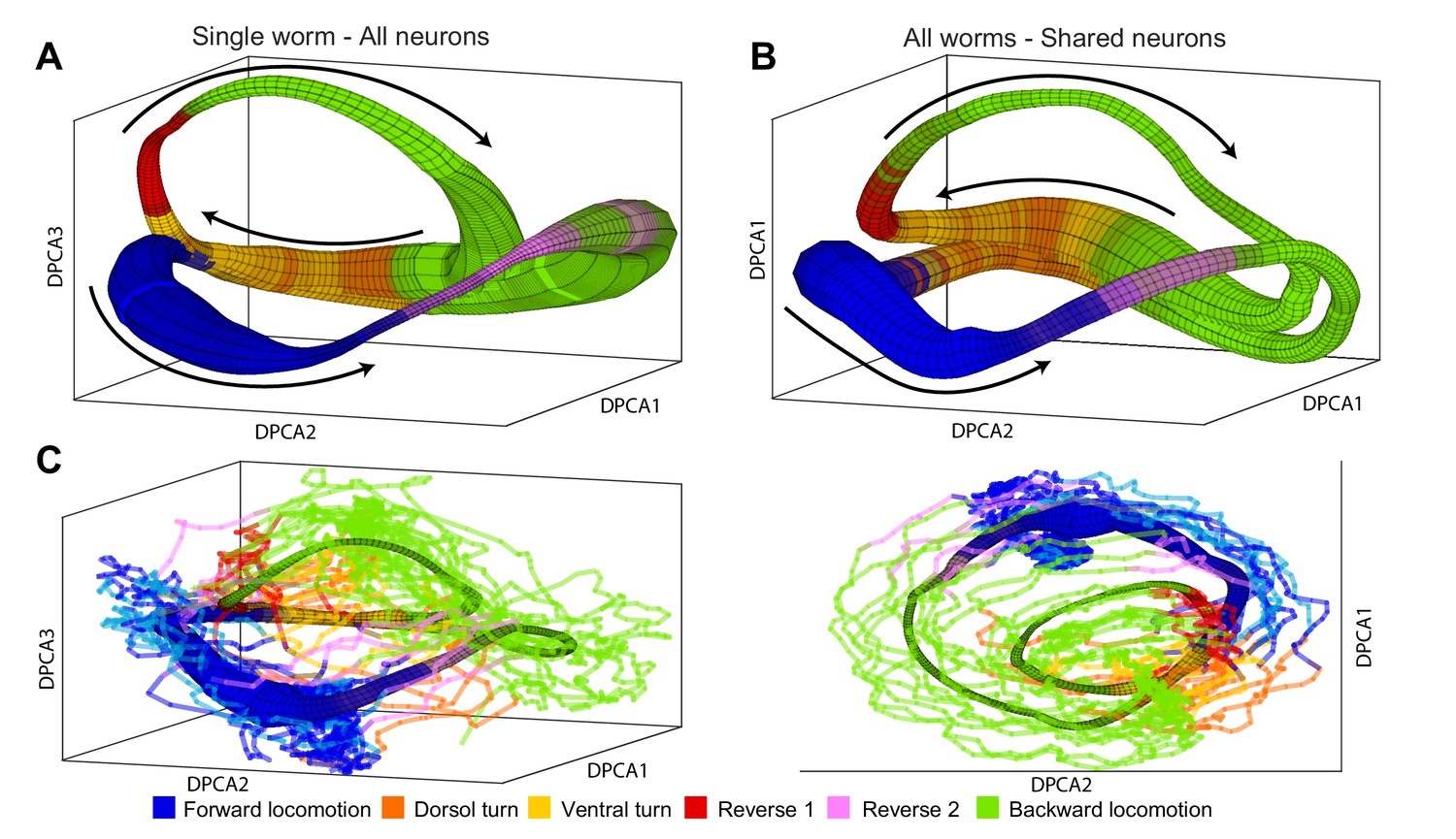
Manifolds are invariant across animals.
(A) Manifold constructed for a single animal using all 107 neurons in the recording. Manifold is color coded according to locomotor behavior assigned to each snapshot of neuronal activity by Kato et al. The prevalence of each behavior in each phase bin is encoded in the opacity of the color for each behavior (colors corresponding to each behavior are shown at bottom of the figure). Black arrows represent the direction of flux around the manifold. DPCA1-3 are the first three principle components of the neuronal activity averaged with respect to and . (B) Manifold constructed using the data from all animals using the 15 shared neurons as common basis. Coloring, projection and arrows are the same as in (A). (C) The data from one animal (lines) is projected onto the manifold constructed from four other animals (surface). The trajectories of the left out animal are well-approximated by the manifold built entirely on the basis of other animals. Behavioral states of the left out animal align well with the distribution of motor commands along the phase of the manifold. This allows us to decode the motor command reliably on the basis of position in manifold space (,) across animals. The same manifold and data is shown in two different projections in order to emphasize the similarities between manifold and data.
Figure 4—figure supplement 1
Projection of calcium imaging data onto DPCAs.
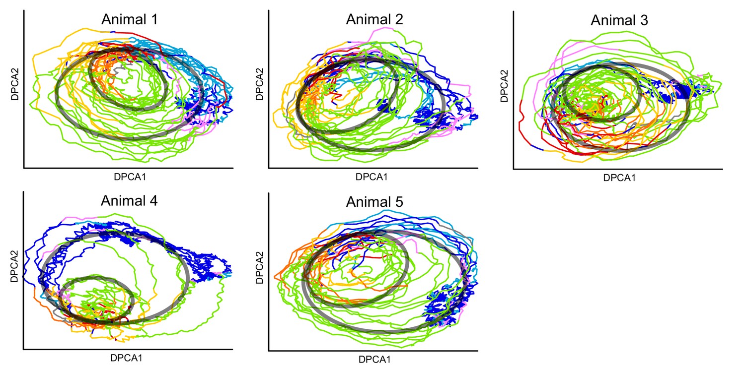
Each animal is projected onto its corresponding first 2 DPCA components after delay embedding using our method from the article. Colors correspond to the fictive behaviors assigned by Kato et al. (2015). Note that the projection of each individual reveals the same two loops that are present in the combined manifold found in the article (Figure 4). The loops are illustrated by the transparent black ovals. Thus, our methodology can be used to uncover loops in neuronal dynamics using ∼100 neurons in each animal. Also see (Figure 4—video 1).
Figure 4—figure supplement 2
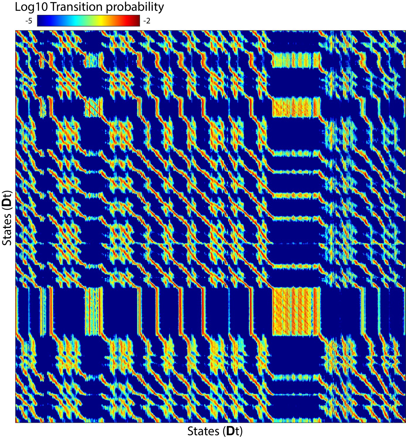
Asymmetric diffusion matrix.
Asymmetric diffusion matrix constructed for a single animal using diffusion kernel as in Equation 13 and normalized such that each row sums to 1 (i.e. a Markov matrix). This matrix was then exponentiated four times to simulate diffusion after ∼1 s. This square matrix has dimensions of the number of time points by the number of time points. Element (, ) corresponds to the probability that a system found in state at time 0 will be in state after 1 s where corresponds to delay embedded neuronal activity. The matrix has two prominent features: patches and diagonal bands. The former correspond to regions in state space where transition probabilities are approximately symmetric and stochastic processes dominate. The latter corresponds to regions where transitions are asymmetric and deterministic flux plays a dominant role.
Figure 4—video 1
Projection of calcium imaging data onto shared DPCAs.
The shared set of 15 neurons recorded in each animal is used to construct a shared DCPA after delay embedding using our method. The video shows the data from all animals projected onto the first 3 components of the shared DPCA. Colors correspond to the fictive behaviors assigned by Kato et al. (2015). The manifold discovered in the main text (Figure 4) is super-imposed on this projection of the data. Note that the assigned behavior of the manifold and the points near a given region of the manifold are in good agreement. Individual behavioral states are segregated to different regions along the manifold. Further, the overall structure of the time series is well described by the same two loops that are found in each individual DPCA projection (Figure 4—figure supplement 1 in contrast to Figure 1—video 1).
Appendix 1—figure 1 with 1 supplement
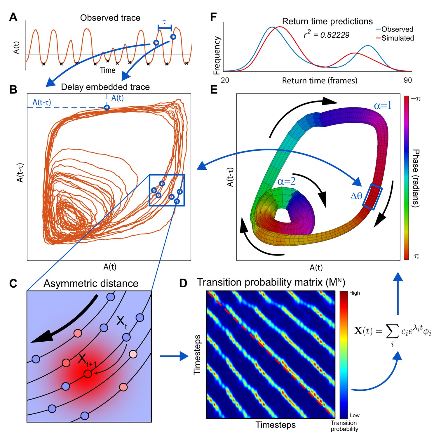
Extraction of manifold from incomplete neuronal activity data.
(A) Observation of a single neuron A) from a two neuron system which produces two distinct modes of oscillation. Activity of at two time points separated by , and (blue dots), is used as x and y coordinates of a single point in the reconstructed phase plane (blue arrows) obtained by delay embedding. (B) When the activity time series in A is projected onto the plane spanned by and , the reconstructed system trajectory reveals two distinct oscillatory cycles present in the complete system. (C) Schematic of asymmetric diffusion map construction. The arrow indicates the direction of preferred flux. Transition probabilities from the state of the system at time , , are computed using a local Gaussian kernel (red high probability; blue low probability). Because this kernel is centered on the next experimentally observed state , transition to is most likely. However, transitions to parallel trajectories (red shows high probability of transition) are also possible. (D) Asymmetrical diffusion map computed for all pairs of states. is sparse because for each point, transition probability is nonzero just for nearest neighbors. Exponentiation of , which shows the evolution of the system after time steps, highlights the asymmetry. The red dashed line shows the main diagonal illustrating that the parallel bands are off center. Eigen-decomposition of the matrix reveals a linear sum of decay equations. is the -th eigenvalue and is the -th eigenvector. represent the initial conditions of the system. (E) Manifold constructed for the two neuron system using only neuron A. Manifold construction method (Materials and methods) uses with the slowest decay time-constant to assign each point in delay embedded space (B) a phase (color of the manifold). identifies position of the system along the cyclic flux. Neuronal activity within a phase bin is averaged such that the center of mass of all points within a bin yields the coordinate of this bin in the delay embedded space. This is used to construct a one-to-one map between a cloud of points in the delay embedded neuronal activity and a phase bin in the manifold space (number of points in each is shown by thickness). Thus, as the system evolves along in the direction given by (black arrows) it traces a trajectory in the delay embedded neuronal activity. Flux separation, accomplished using cluster analysis, assures that similar phases of different fluxes are not mistakenly grouped together (Materials and methods). (F) Simulations of the manifold in the phase space (, ) recapitulate neuronal activation. To show this we compare the simulated distribution of time intervals between consecutive minima of A (return times) and those produced by the full system including both neurons (minima shown by black Xs in A).
Appendix 1—figure 1—figure supplement 1

State space and flux in dynamical systems with noise.
(A) Network diagram of the two neuron toy system explored in the paper. ‘Excitatory’ neuron synapses (red triangle) onto ‘inhibitory’ neuron which synapses (blue triangle) back onto neuron . (B) Simulation of the two neuron system with noise. Red and blue traces show activity of neuron and respectively. (C) Black arrows represent the flux for positions in the state space (, ). Lines represent trajectories spanned by the state of the system as it evolves in time without noise. Trajectories either converge onto the outer loop (purple) or onto the inner loop (green) over time. These two loops are the cyclic fluxes of the system. (D) Adding noise to the system causes the trajectories to tangle and stochastically switch between the inner and outer cyclic fluxes. Nonetheless, the probability density of points is predominantly concentrated around the two cyclic fluxes and evolves in the same direction as in the system without noise.
Tables
Appendix 1—table 1
Parameters used in model construction of C. elegans dynamics.
https://doi.org/10.7554/eLife.46814.021| Parameter name | Parameter value | Parameter description |
|---|---|---|
| Number of neighbors | 12 | number of nearest trajectories in a local neighborhood |
| Minimum time frame | 50 | minimum time separation for nearest trajectories |
| Number of delays | 5 | Number of times the neuronal activity was embedded |
| Delay length | 10 | in units of number of frames |
Additional files
-
Transparent reporting form
- https://doi.org/10.7554/eLife.46814.017
Download links
A two-part list of links to download the article, or parts of the article, in various formats.
Downloads (link to download the article as PDF)
Open citations (links to open the citations from this article in various online reference manager services)
Cite this article (links to download the citations from this article in formats compatible with various reference manager tools)
A quantitative model of conserved macroscopic dynamics predicts future motor commands
eLife 8:e46814.
https://doi.org/10.7554/eLife.46814


