Consistent and correctable bias in metagenomic sequencing experiments
- North Carolina State University, United States
- University of Washington, United States
Figures
Figure 1

Bias arises throughout an MGS workflow, creating systematic error between the observed and actual compositions.
Panel A illustrates a hypothetical marker-gene measurement of an even mixture of three taxa. The observed composition differs from the actual composition due to the bias at each step in the workflow. Panel B illustrates our mathematical model of bias, in which bias multiplies across steps to create the bias for the MGS protocol as a whole.
Figure 2
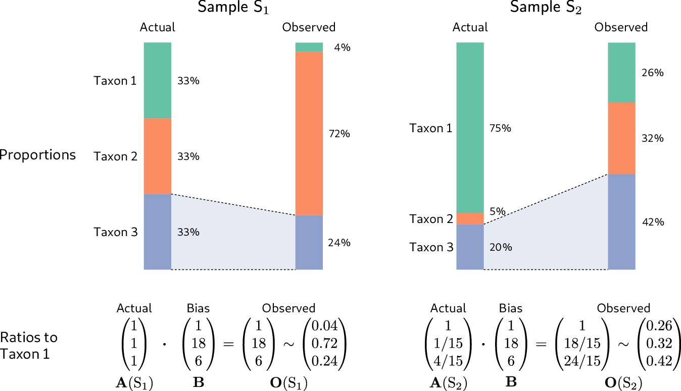
Consistent multiplicative bias causes systematic error in taxon ratios, but not taxon proportions, that is independent of sample composition.
The even community from Figure 1 and a second community containing the same three taxa in different proportions are measured by a common MGS protocol. Measurements of both samples are subject to the same bias, but the magnitude and direction of error in the taxon proportions depends on the underlying composition (top row). In contrast, when the relative abundances and bias are both viewed as ratios to a fixed taxon (here, Taxon 1), the consistent action of bias across samples is apparent (bottom row).
Figure 3 with 3 supplements
Our model of bias explains the systematic error observed in the Brooks et al. (2015) cell-mixture experiment.
The top row compares the observed proportions of individual taxa to the actual proportions (Panel A) and to those predicted by our fitted bias model (Panel B). Panel A shows significant error across all taxa and mixture types that is almost entirely removed once bias is accounted for in Panel B. Panel C shows the observed error in proportions of individual taxa, while Panel D shows the error in the ratios of pairs of taxa for five of the seven taxa. The ratio predicted by the fitted model is given by the black cross in Panel D. As predicted by our model, the error in individual proportions (Panel C) depends highly on sample composition, while the error in ratios (Panel D) does not.
Figure 3—figure supplement 1
The observed error in taxon ratios for all three mixture experiments.
The observed error in taxon ratios (colored dots) against the fitted model prediction (black cross) for the three mixture experiments of Brooks et al. (2015).
Figure 3—figure supplement 2

Observed vs. expected proportions under no bias, copy-number bias only, and the estimated bias.
Comparison of the observed proportions with three types of expected proportions—the actual proportions, the proportions predicted from the estimated 16S copy numbers in Table 3, and the proportions predicted by the fitted bias model—for the three mixture experiments of Brooks et al. (2015). Proportions are transformed to log-odds () to avoid compressing errors near and , and average mean squared error (MSE) of the log-odds are shown.
Figure 3—figure supplement 3
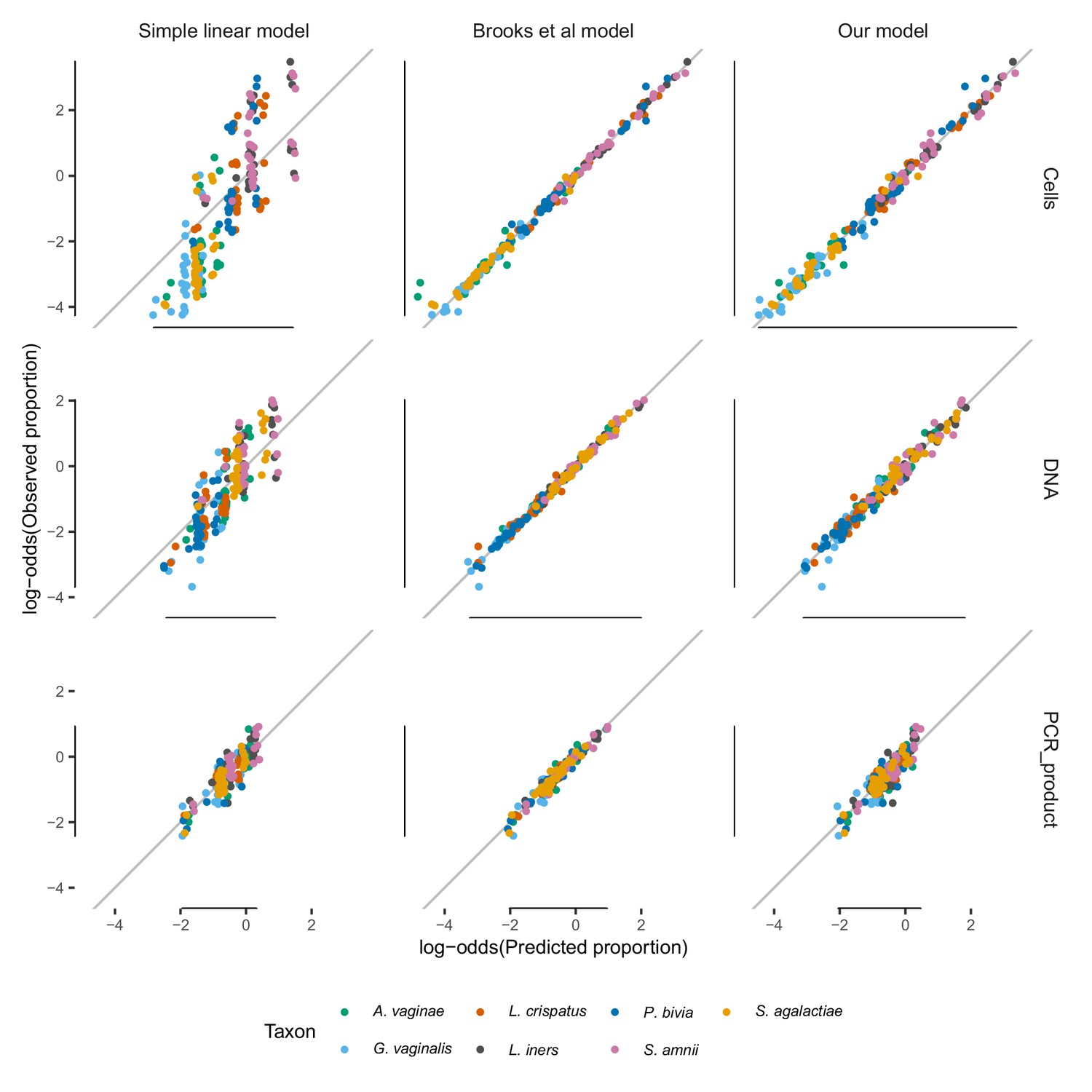
Comparison between the simple linear model, the linear interactions model of Brooks et al. (2015), and our model.
Comparison of the model fits for the simple linear model, the linear interactions model of Brooks et al. (2015), and our model. The simple linear model has a poor fit, while the Brooks et al. (2015) model closely fits the data but does so by having more parameters per taxon (63 per taxon) than distinct sample compositions (58). Our model fits nearly as well as the Brooks et al. (2015) model for the Cells and DNA mixtures, while having vastly fewer parameters (6 versus 441 for all taxa). Proportions are transformed to log-odds () to avoid compressing errors near and . The simple linear model with and without an intercept term gives nearly identical results except near zero; here shown without. Only taxa with non-zero actual abundance are plotted, and proportions predicted to be greater than one by the simple linear model are not shown.
Figure 4 with 1 supplement
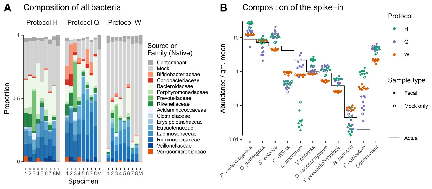
Bias of the mock spike-in in the Costea et al. (2017) experiment is consistent across samples with varying background compositions.
Panel A shows the variation in bacterial composition across protocols and specimens (Labels 1 through 8 denote fecal specimens; M denotes the mock-only specimen) and Panel B shows the relative abundance of the 10 mock taxa and the spike-in contaminant (dots) against the actual composition (black line). In Panel A, color indicates source (mock, contaminant, or native gut taxon) and Family for native bacterial taxa with a proportion of 0.02 in at least one sample. Families are colored by phylum (Red: Actinobacteria, Green: Bacteroidetes, Blue: Firmicutes, Orange: Verrucomicrobia). In Panel B, abundance is divided by the geometric mean of the mock (non-contaminant) taxa in that sample.
Figure 4—figure supplement 1
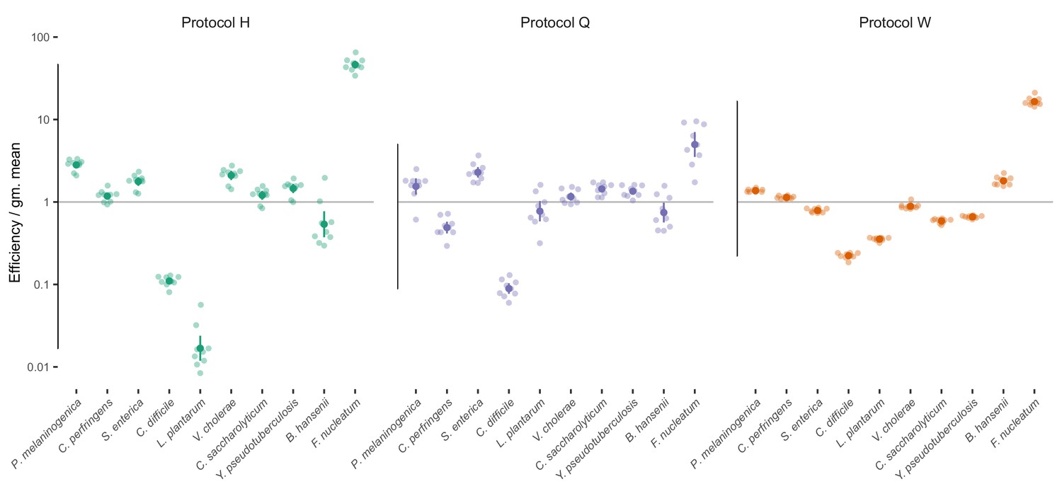
Estimated bias for the mock taxa for the three protocols.
Estimated bias for the 10 mock taxa for the three protocols in the Costea et al. (2017) experiment. Bias is shown as relative to the average taxon; that is, the efficiency of each taxon is divided by the geometric mean efficiency of all taxa. The estimated efficiencies are shown as the best estimate (dark dot) multiplied and divided by two geometric standard errors (lines), along with the observations from individual samples (translucent dots).
Figure 5 with 1 supplement
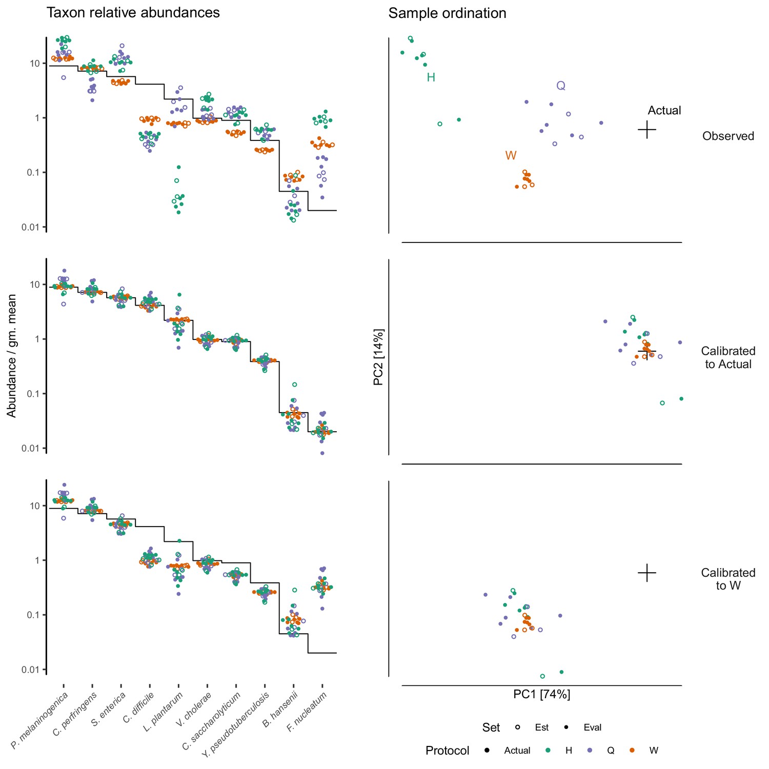
Calibration can remove bias and make MGS measurements from different protocols quantitatively comparable.
For the sub-community defined by the mock spike-in of the Costea et al. (2017) dataset, we estimated bias from three specimens (the estimation set ‘Est’) and used the estimate to calibrate all specimens. The left column shows taxon relative abundances as in Figure 4B and the right column shows the first two principal components from a compositional principle-components analysis (Gloor et al., 2017). The top row shows the measurements before calibration; the middle, after calibration to the actual composition; and the bottom, after calibration to Protocol W.
Figure 5—figure supplement 1
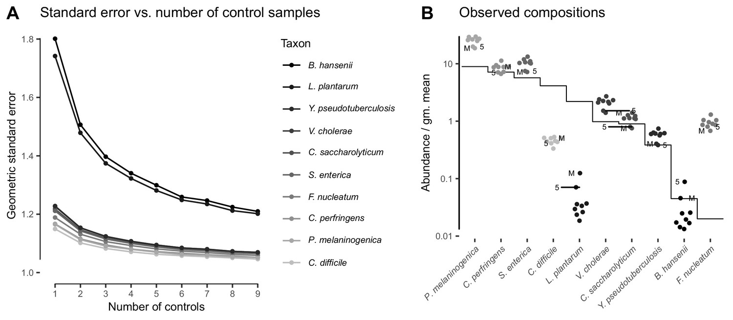
Precision in the bias estimate vs. the number of control samples for Protocol H.
Precision in bias estimate decreases with the number of control samples and depends on the noise associated with each taxon. For Protocol H in the Costea et al. (2017) experiment, Panel A shows the geometric standard error in the relative efficiencies of the 10 mock taxa (which jointly form the estimated bias) versus the number of control samples used to estimate the bias. As elsewhere, the efficiency of each taxon is divided by the geometric mean efficiency of all 10 mock taxa. Panel B shows the observed against the actual relative abundances, as in Figure 4. The two marked samples (from Individual 5 and the mock-only sample M) have unusually high observed abundances of L. plantarum and B. hansenii and are largely responsible for the much higher standard error seen for these two taxa.
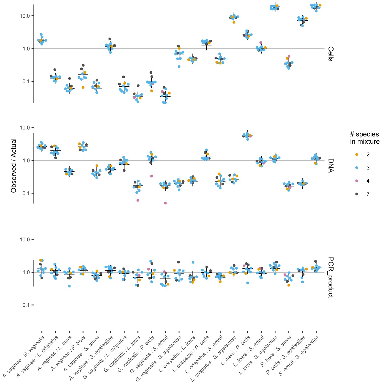
Figure 6 with 1 supplement
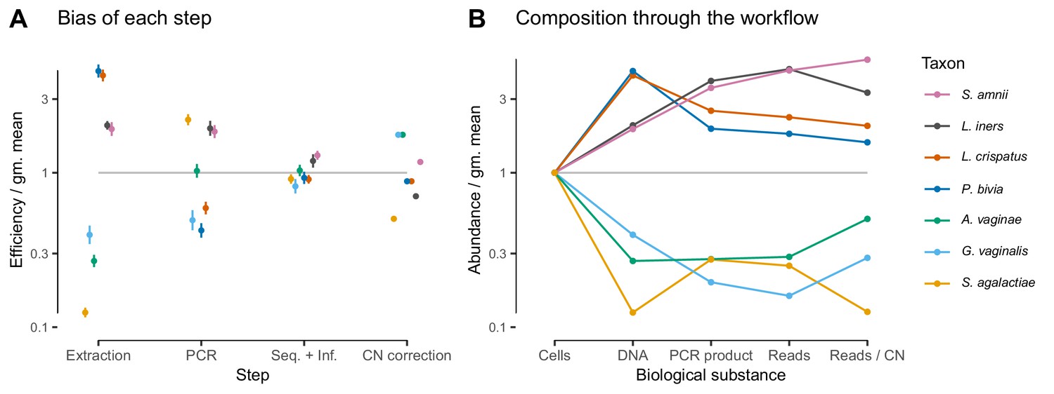
In the Brooks et al. (2015) experiment, bias is primarily driven by DNA extraction and is not substantially reduced by 16S copy-number (CN) correction.
Panel A shows the bias estimate for each step in the experimental workflow (DNA extraction, PCR amplification, and sequencing + (bio)informatics), as well as the bias imposed by performing 16S CN correction (i.e. dividing by the estimated number of 16S copies per genome). Bias is shown as relative to the average taxon—that is, the efficiency of each taxon is divided by the geometric mean efficiency of all seven taxa—and the estimated efficiencies are shown as the best estimate multiplied and divided by two geometric standard errors. Panel B shows the composition through the workflow, starting from an even mixture of all seven taxa, obtained by sequentially multiplying the best estimates in Panel A.
Figure 6—figure supplement 1
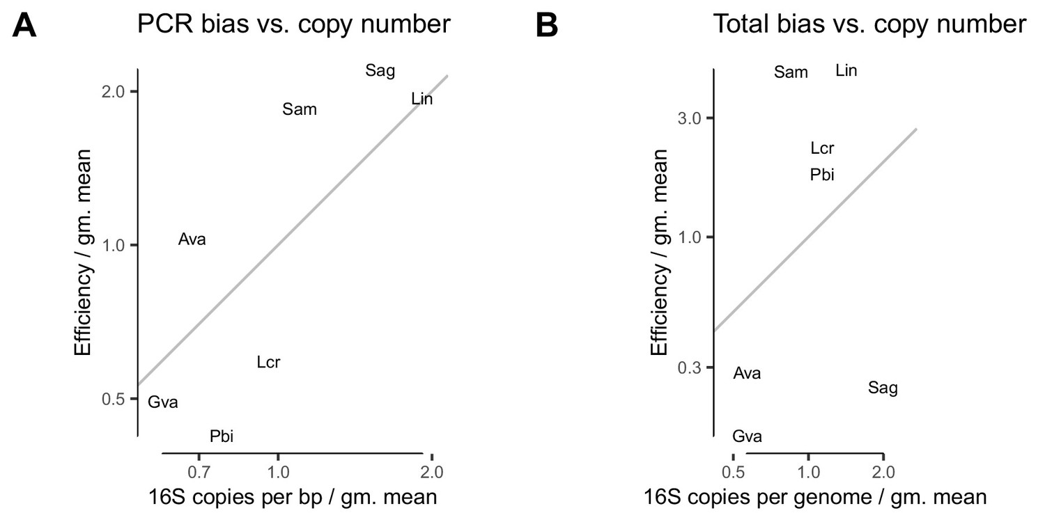
PCR bias and total bias vs. bias predicted by 16S copy number.
In the Brooks et al. (2015) experiment, variation in 16S copy number is moderately predictive of PCR bias (A) but not of total bias (B). The grey line corresponds to , or perfect agreement between CN and the estimated bias.
Author response image 1
Tables
Table 1
Estimated bias for the three Brooks et al. (2015) mixture experiments.
The first three columns show the bias estimated in each mixture experiment; the second three columns show the bias estimated for individual protocol steps from the mixture estimates. In each case, bias is shown as relative to the average taxon; that is, the efficiency of each taxon is divided by the geometric mean efficiency of all seven taxa. The last three rows summarize the multiplicative error in taxon ratios due to bias and noise. Taxa are ordered by decreasing efficiency in the cell mixtures. Abbreviations: PCR prod.: PCR product; Seq. + Inf.: Sequencing + Informatics.
| Mixtures | Steps | |||||
|---|---|---|---|---|---|---|
| Taxon | Cells | DNA | PCR prod. | Extraction | PCR | Seq.+Inf. |
| Lactobacillus iners | 4.7 | 2.3 | 1.2 | 2.0 | 1.9 | 1.2 |
| Sneathia amnii | 4.6 | 2.4 | 1.3 | 1.9 | 1.8 | 1.3 |
| Lactobacillus crispatus | 2.3 | 0.5 | 0.9 | 4.3 | 0.6 | 0.9 |
| Prevotella bivia | 1.8 | 0.4 | 0.9 | 4.6 | 0.4 | 0.9 |
| Atopobium vaginae | 0.3 | 1.1 | 1.0 | 0.3 | 1.0 | 1.0 |
| Streptococcus agalactiae | 0.2 | 2.0 | 0.9 | 0.1 | 2.2 | 0.9 |
| Gardnerella vaginalis | 0.2 | 0.4 | 0.8 | 0.4 | 0.5 | 0.8 |
| Max pairwise bias | 29.3 | 6.1 | 1.6 | 36.6 | 5.2 | 1.6 |
| Avg. pairwise bias | 5.6 | 2.7 | 1.2 | 5.5 | 2.3 | 1.2 |
| Avg. pairwise noise | 1.2 | 1.2 | 1.3 | — | — | — |
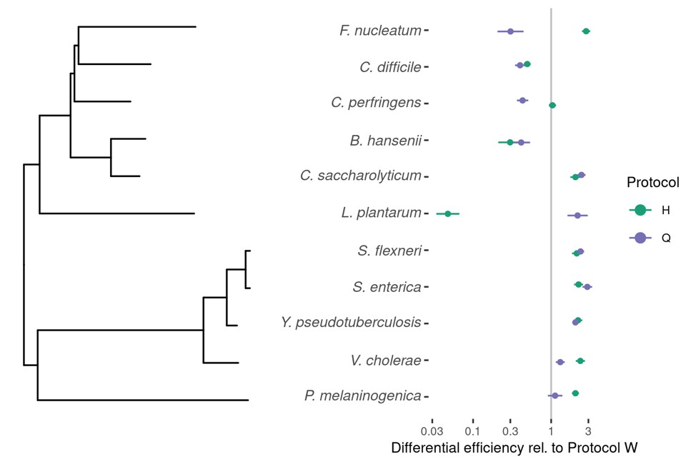
Table 2
Estimated bias and differential bias among the spike-in taxa for the three protocols (Protocols H, Q, and W) in the Costea et al. (2017) experiment.
The first three columns show the bias of the given protocol for the 10 mock taxa; the second three columns show the differential bias between protocols for the 10 mock taxa and the contaminant. In each case, bias is shown as relative to the average mock (non-contaminant) taxon; that is, the efficiency of each taxon is divided by the geometric mean efficiency of the 10 mock taxa. The last three rows summarize the multiplicative error in taxon ratios due to bias and noise; the contaminant is excluded from these statistics to allow direct comparison between bias and differential bias. Taxa are ordered as in Figure 4B.
| Protocol | Protocol/Reference | |||||
|---|---|---|---|---|---|---|
| Taxon | H | Q | W | H/Q | H/W | Q/W |
| Prevotella melaninogenica | 2.81 | 1.55 | 1.37 | 1.82 | 2.05 | 1.12 |
| Clostridium perfringens | 1.18 | 0.49 | 1.14 | 2.41 | 1.04 | 0.43 |
| Salmonella enterica | 1.77 | 2.29 | 0.79 | 0.77 | 2.25 | 2.90 |
| Clostridium difficile | 0.11 | 0.09 | 0.22 | 1.24 | 0.49 | 0.40 |
| Lactobacillus plantarum | 0.02 | 0.77 | 0.35 | 0.02 | 0.05 | 2.18 |
| Vibrio cholerae | 2.10 | 1.16 | 0.89 | 1.81 | 2.37 | 1.31 |
| Clostridium saccharolyticum | 1.21 | 1.44 | 0.59 | 0.84 | 2.05 | 2.45 |
| Yersinia pseudotuberculosis | 1.46 | 1.35 | 0.66 | 1.08 | 2.21 | 2.05 |
| Blautia hansenii | 0.54 | 0.74 | 1.80 | 0.72 | 0.30 | 0.41 |
| Fusobacterium nucleatum | 46.29 | 4.98 | 16.51 | 9.30 | 2.80 | 0.30 |
| Contaminant | — | — | — | 0.89 | 2.13 | 2.38 |
| Max pairwise bias | 2751 | 56 | 74 | 428 | 59 | 10 |
| Avg. pairwise bias | 9.7 | 3.2 | 3.5 | 4.7 | 3.9 | 2.8 |
| Avg. pairwise noise | 1.3 | 1.5 | 1.1 | 1.5 | 1.3 | 1.5 |
Table 3
Estimated genome size and 16S copy number for the seven mock taxa in the Brooks et al. (2015) experiment (Materials and methods).
https://doi.org/10.7554/eLife.46923.016| Taxon | Genome size (Mbp) | Copy number |
|---|---|---|
| Atopobium vaginae | 1.44 | 2* |
| Gardnerella vaginalis | 1.64 | 2 |
| Lactobacillus crispatus | 2.04 | 4 |
| Lactobacillus iners | 1.28 | 5* |
| Prevotella bivia | 2.52 | 4* |
| Sneathia amnii | 1.33 | 3* |
| Streptococcus agalactiae | 2.16 | 7 |
-
*Denotes copy numbers that were instead estimated to be 1 by Brooks et al. (2015).
Additional files
-
Transparent reporting form
- https://doi.org/10.7554/eLife.46923.017
Download links
A two-part list of links to download the article, or parts of the article, in various formats.
Downloads (link to download the article as PDF)
Open citations (links to open the citations from this article in various online reference manager services)
Cite this article (links to download the citations from this article in formats compatible with various reference manager tools)
Consistent and correctable bias in metagenomic sequencing experiments
eLife 8:e46923.
https://doi.org/10.7554/eLife.46923


