Inferring synaptic inputs from spikes with a conductance-based neural encoding model
- University of Washington, United States
- Princeton University, United States
Figures
Figure 1 with 1 supplement
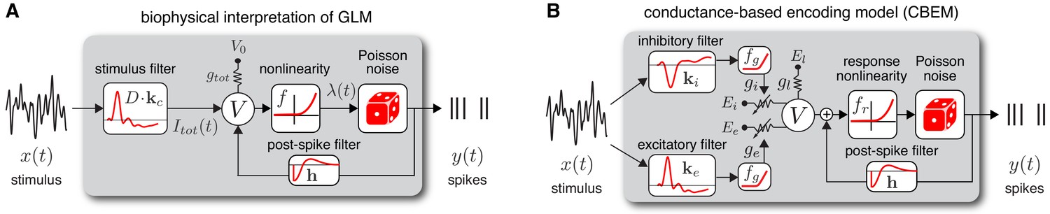
Model diagrams.
(A) Diagram illustrating novel biophysical interpretation of the generalized linear model (GLM). The stimulus is convolved with a conductance filter weighted by , the difference between excitatory and inhibitory current reversal potentials, resulting in total synaptic current . This current is injected into the linear RC circuit governing the membrane potential , which is subject to a leak current with conductance and reversal potential . The instantaneous probability of spiking is governed by a the conditional intensity , where is a nonlinear function with non-negative output. Spiking is conditionally Poisson with rate , and spikes gives rise to a post-spike current or filter that affects the subsequent membrane potential. (B) Conductance-based encoding model (CBEM). The stimulus is convolved with filters and , whose outputs are transformed by rectifying nonlinearity to produce excitatory and inhibitory synaptic conductances and . These time-varying conductances and the static leak conductance drive synaptic currents with reversal potentials , , and , respectively. The resulting membrane potential is added to a linear spike-history term, given by , and then transformed via rectifying nonlinearity to obtain the conditional intensity , which governs conditionally Poisson spiking as in the GLM. Figure 1—figure supplement 1 shows that the CBEM parameters can be recovered from simulated data.
Figure 1—figure supplement 1
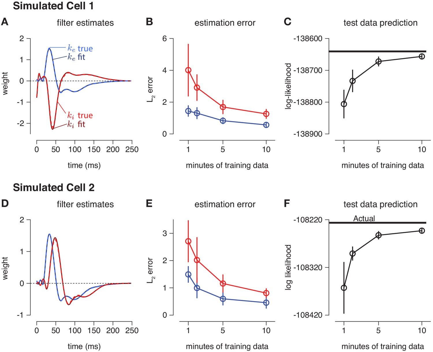
Convergence of model parameter fits.
(A) Estimates (solid traces) of excitatory (blue) and inhibitory (red) filters from 10 min of simulated spike trains. (Dashed lines indicate true filters). The inhibitory filter was oppositely tuned and delayed compared to the excitatory filter. (B) The norm between the estimated input filters and the true filters as a function of the amount of training data. (C) The log-likelihood of the fit CBEM on the test data converged towards the log-likelihood of the true model. (D,E,F) Same as A-C for a simulation in which had the same tuning as with a delay.
Figure 2
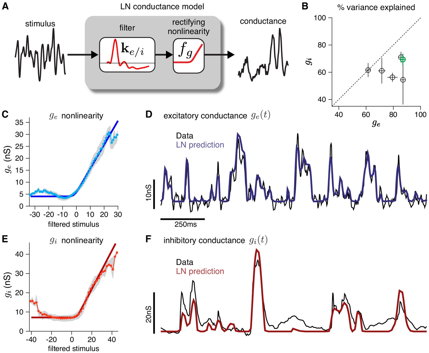
Validating the LN conductance model.
The CBEM describes the relationship between stimulus and each synaptic conductance with a linear-nonlinear (LN) cascade, consisting of a linear filter followed by a fixed rectifying nonlinearity. (A) LN conductance model schematic. (B) The percent variance explained () for excitatory and inhibitory conductances from 6 ON parasol RGCs, computed using cross-validation with a 6 s test stimulus. Error bars indicate standard deviation across all test stimuli. (C) The excitatory conductance as a function of the filtered stimulus values for the example cell indicated in green in B. The gray region shows the middle 50-percentile of the distribution of observed excitatory conductance given the filtered stimulus value. The soft-rectifying nonlinearity (dark blue) closely matched the average conductance given the filtered stimulus value (light blue points). (D) Measured excitatory conductances in the same cell (black) and predictions from the LN model (blue) in response to a test stimulus. (E) The inhibitory conductance nonlinearity for the same neuron. The soft-rectifying nonlinearity (dark red) closely approximated the average inhibitory conductance as a function of the filtered stimulus value (light red). (F) Measured excitatory conductances (black) and the predictions of the LN model (red) on a test stimulus for the same cell.
Figure 3
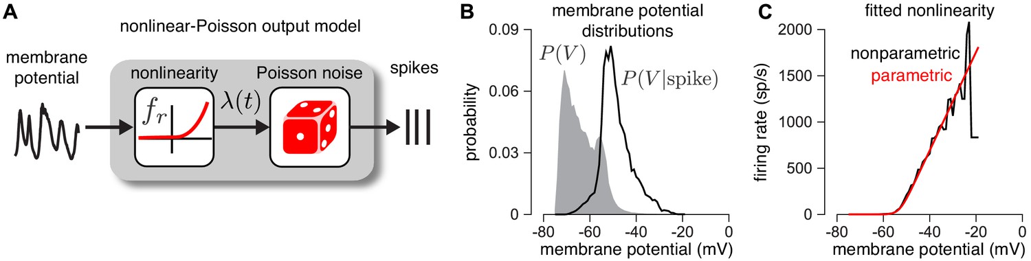
Validating the firing rate nonlinearity.
(A) Schematic of the mapping from membrane potential to spikes under the CBEM. (B) The raw (gray) and spike-triggered (black) distribution of intracellular membrane potential obtained from intracellular recordings in two parasol RGCs. (C) Nonparametric estimate of the output nonlinearity (black trace), computed by applying Bayes’ rule to the distributions in B, compared to a soft-rectified linear function (red trace).
Figure 4
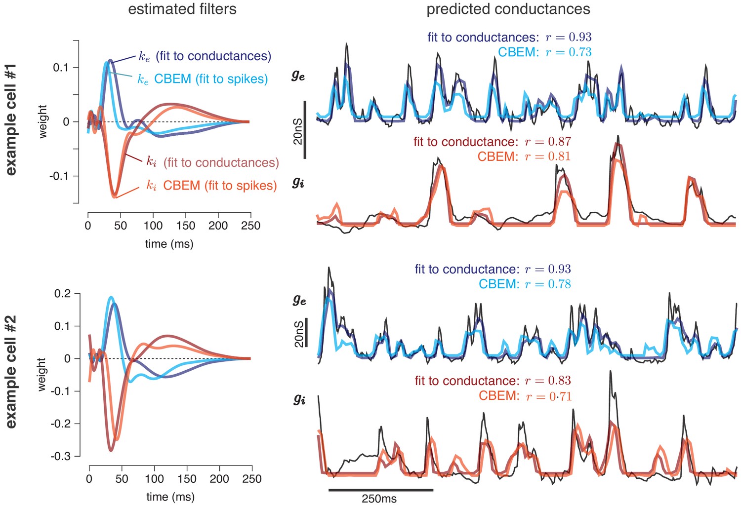
Predicting conductances from spikes with CBEM.
Model parameters and conductance predictions for two example ON parasol RGCs. Left: Linear kernels for the excitatory (blue) and inhibitory (red) conductances estimated from spike train data (light red, light blue) alongside filters from an LN model fit directly to measured conductances (dark red, dark blue). The filters represent a combination of events that occur in the retinal circuitry in response to a visual stimulus, and are primarily shaped by the cone transduction process. Right: Measured conductances elicited by a test stimulus (black), along with predictions from the CBEM (fit to spikes) and LN model (fit to conductance data), indicating that the CBEM can predict synaptic conductances nearly as well as a model fit to intracellular conductance measurements. Estimated conductances and conductance filters are scaled for ease of visualization due to the presence of an unidentifiable scale factor relating to membrane capacitance. Inhibition and excitation were scaled equally.
Figure 5
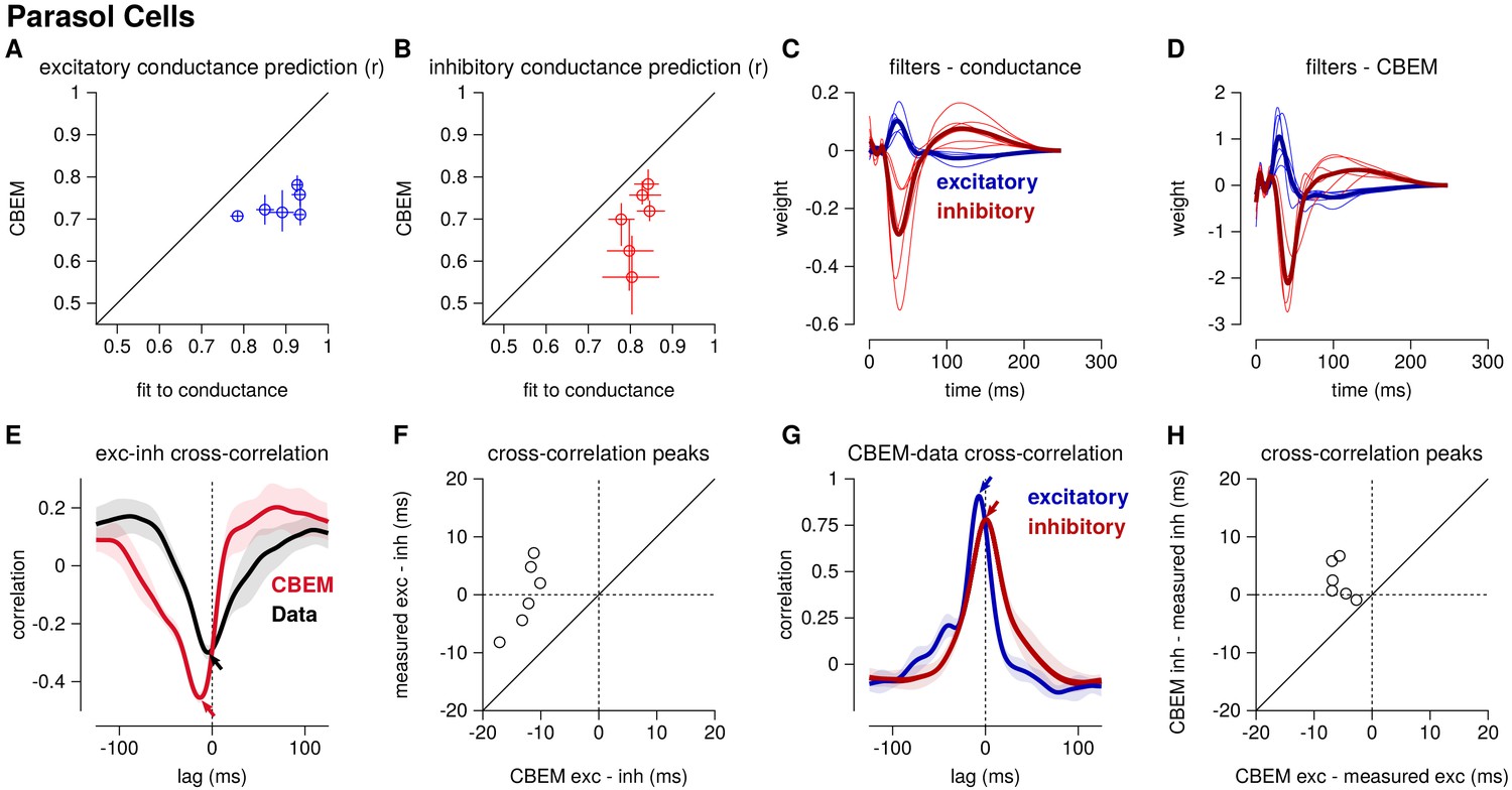
Summary of the CBEM fits to 6 ON parasol RGCs for which we had both spike train and conductance recordings.
(A) The correlation coefficient () between the mean observed excitatory synaptic input to a novel 6 s stimulus and the conductance predicted by the LN cascade fit to the excitatory conductance (y-axis) compared to the CBEM prediction from spikes (x-axis) for each cell. Error bars indicate the minimum and maximum values observed across all cross-validated stimuli (B) Same as C for the inhibitory conductance. (C) The excitatory (blue) and inhibitory (red) filters estimated from voltage-clamp recordings. The thick traces show the mean filters. (D) The excitatory (blue) and inhibitory (red) filters estimated by the CBEM from spike trains. (E) The cross-correlation of the excitatory and inhibitory conductances for an example cell measured from the data (black trace; region shows standard deviation across the 10 stimuli) compared to the cross-correlation in the CBEM fit to that cell (red trace). Arrows indicate the peaks of the cross-correlations. In the data, excitation and inhibition are anti-correlated and show similar timing. However, excitation precedes inhibition in the model. (F) The cross-correlation peak times between excitation and inhibition measured from data (y-axis) compared to the conductances predicted by the CBEM (x-axis) for all 6 cells. Negative values on the x-axis indicate that excitation leads inhibition in the CBEM fits to these cells. (G) Comparing the timing of excitatory and inhibitory conductances from the data and the CBEM for the example cell in E. The cross-correlation between the measured excitatory conductance and the CBEM’s excitatory conductance (blue) and the cross-correlation between data and model for the inhibitory conductances (red). (H) Cross-correlation peak times between measured and CBEM predicted inhibition (y-axis) and excitation (x-axis).
Figure 6 with 1 supplement

Summary of the CBEM fits to 5 ON midget RGCs.
The plot follows the same conventions as the parasol results in Figure 5. (A,B) The correlation coefficient () between the mean observed excitatory and inhibitory synaptic input to a novel 6 s stimulus and the conductance predicted by the LN cascade fit to the excitatory conductance (y-axis) compared to the CBEM prediction from spikes (x-axis) for each cell. Conductance predictions for a single example cell are shown in Figure 6—figure supplement 1. The excitatory (blue) and inhibitory (red) filters estimated from voltage-clamp recordings (C) and by the CBEM from spike trains (D). (E) The cross-correlation of the excitatory and inhibitory conductances for an example cell measured from the test stimulus (data) compared to the cross-correlation predicted by the CBEM fit to that cell (red trace). (F) The cross-correlation peak times between excitation and inhibition measured from data compared to the conductances predicted by the CBEM for all five cells. (G) Comparing the timing of excitatory and inhibitory conductances from the data and the CBEM for the example cell in E. The cross-correlation between the measured excitatory conductance and the CBEM’s excitatory conductance (blue) and the cross-correlation between data and model for the inhibitory conductances (red). (H) Cross-correlation peak times between measured and CBEM predicted inhibition and excitation.
Figure 6—figure supplement 1
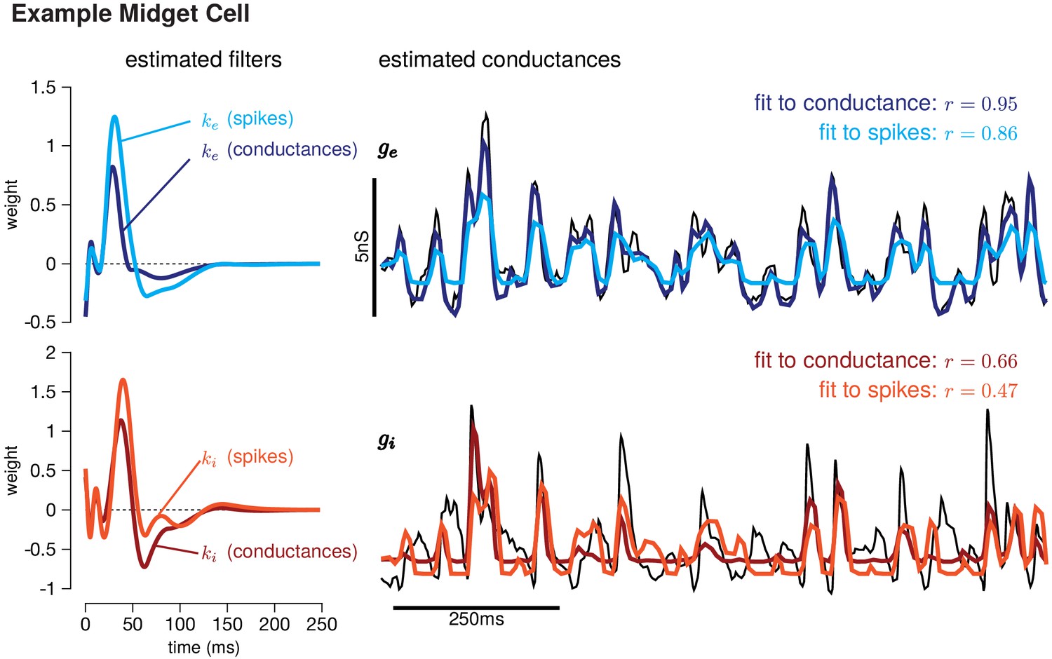
CBEM fit for an example ON-midget cell with a comparison the LN models fit directly to the conductances.
Left: Linear kernels for the excitatory (blue) and inhibitory (red) inputs estimated from the conductance-based model (light red, light blue) and estimated by fitting a linear-nonlinear model directly to the measured conductances (dark red, dark blue). The filters represent a combination of events that occur in the retinal circuitry in response to a visual stimulus, and are primarily shaped by the cone transduction process. Right: Conductances predicted by our model on a withheld test stimulus. Measured conductances (black) are compared to the predictions from the CBEM filters (fit to spiking data) and an LN model (fit to conductance data). For visualization, we scaled the estimated conductances from the CBEM as in Figure 4.
Figure 7 with 1 supplement
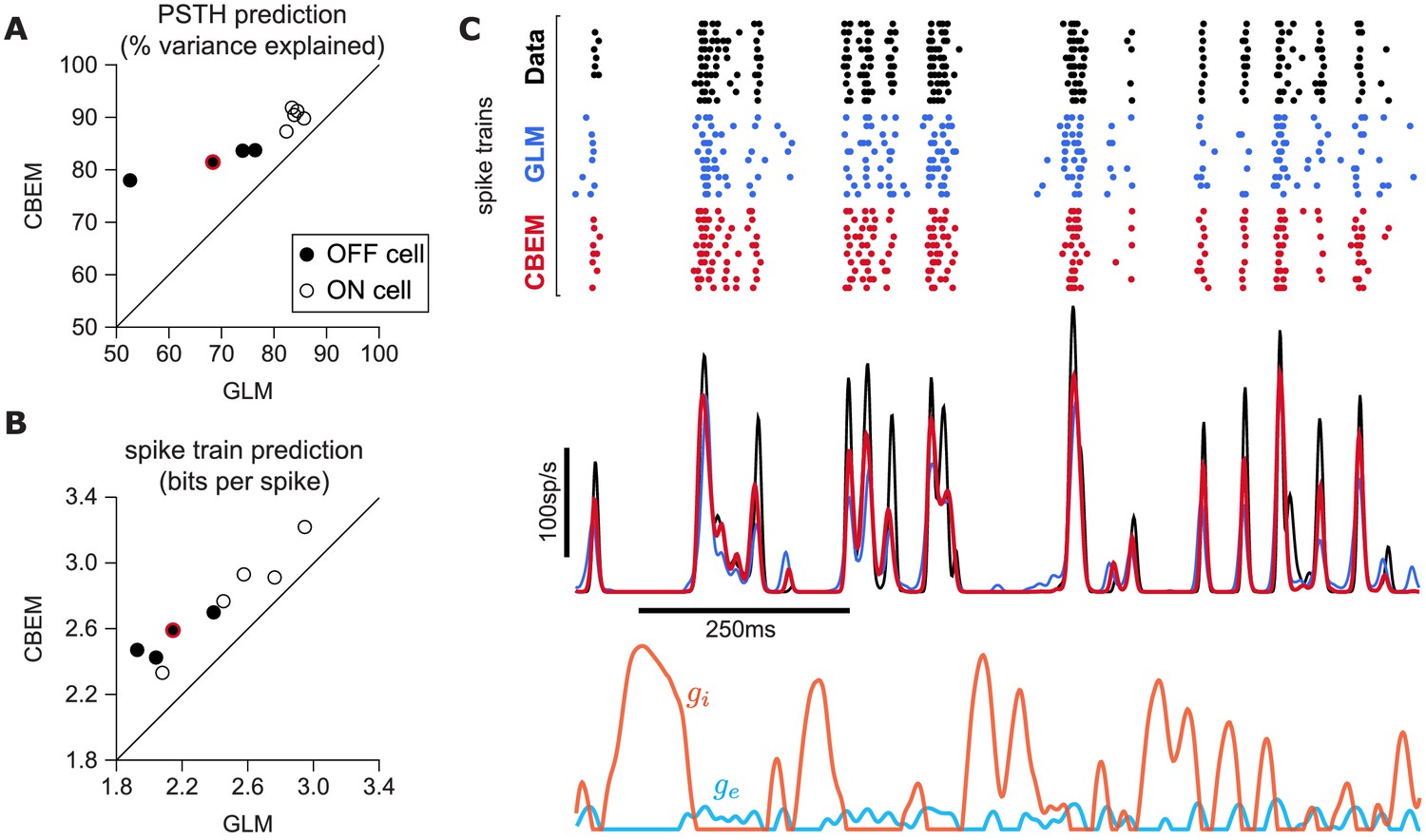
CBEM spike train predictions.
(A) Spike rate prediction performance for the population of nine cells for 5 s test stimulus. The true rate (black) was estimated using 167 repeat trials. The red circle indicates the cell shown in C. (B) Log-likelihood of the CBEM compared to the GLM computed on a 5 min test stimulus. (C) (top) Raster of responses of an example OFF parasol RGC to repeats of a novel stimulus (black) and simulated responses from the GLM (blue) and the CBEM (red). (middle) Spike rate (PSTH) of the RGC and the GLM (blue) and CBEM (red). The PSTHs were smoothed with a Gaussian kernel with a 2 ms standard deviation. (bottom) The CBEM predicted excitatory (blue) and inhibitory (orange) conductances. The conductances are given in arbitrary units because the model does not include membrane capacitance. Figure 7—figure supplement 1 CBEM conductance predictions.
Figure 7—figure supplement 1
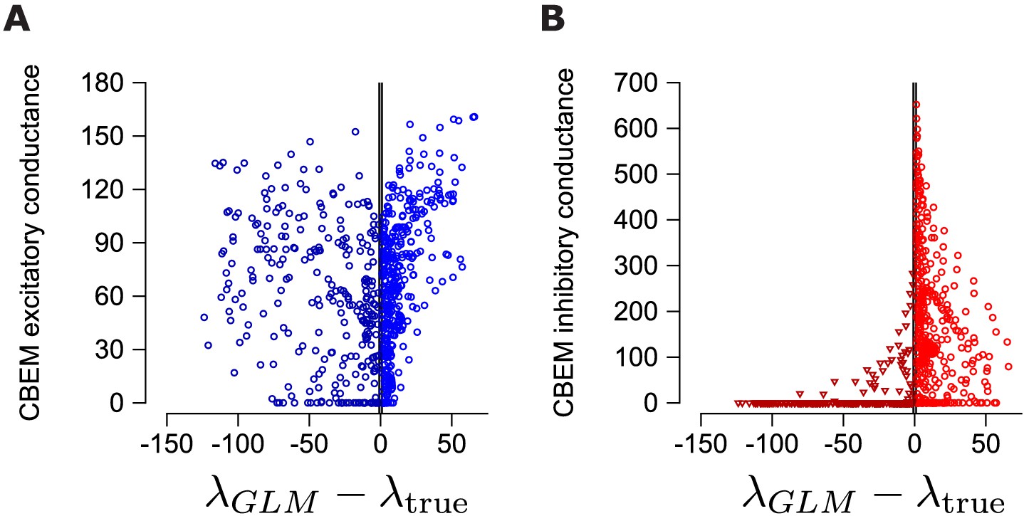
Relation of inferred conductances to GLM prediction error.
(A) The difference in the GLM predicted rate () and the measure spike rate () from the PSTH in Figure 7c compared to the excitatory conductances predicted by the CBEM. We only considered the time points for which the predicted rate and the measured rate differed by at least one spike/s (gray region denotes the eliminated interval). (B) Same as A for the inhibitory conductance.
Figure 8

Comparison of CBEM and GLM fits.
(A) Spike rate prediction performance and (B) cross-validated log-likelihood for the population of nine cells for 7 s test stimulus for the GLM and the CBEM with only an excitatory input term (CBEMexc). (C) The full CBEM with inhibition shows improved spike rate predication and (D) cross-validated log-likelihood compared to the model without inhibition. (E) The GLM filters for nine parasol RGCs (black) compared to the excitatory conductance filters estimated by the CBEM without an inhibitory input (blue). The GLM filters are shown scaled to match the height of the CBEMexc filters.
Figure 9 with 2 supplements

Contrast gain control in the CBEM.
(A) GLM filters for an example ON cell fit to responses recorded at 24%, 48%, and 96% contrast. (B) GLM filters fit to spike trains simulated from the CBEM fit to the cell shown in A. The CBEM was fit to responses at all three contrast levels. Filter height comparisons for CBEM fits to all cells are shown in Figure 9—figure supplement 1. Spike train prediction performance of the (C) GLM and (D) the CBEM tested on a 4 min stimulus at 24% (left column), 48% (middle column), and 96% (right column) contrast. The model trained on all three contrast levels (y-axis) is plotted against the same class of model trained only at the probe contrast level (x-axis). Figure 9—figure supplement 2 shows the cross-correlation between the CBEM predicted excitation and inhibition over a range of contrasts.
Figure 9—figure supplement 1

The filter heights (the absolute value of the peak of the filter) of the GLM fits to eight cells at all three contrast levels (one point per contrast level per cell; lines connect all contrast points from a cell), compared to the GLM filters fit the CBEM simulations of those same cells.
Figure 9—figure supplement 2
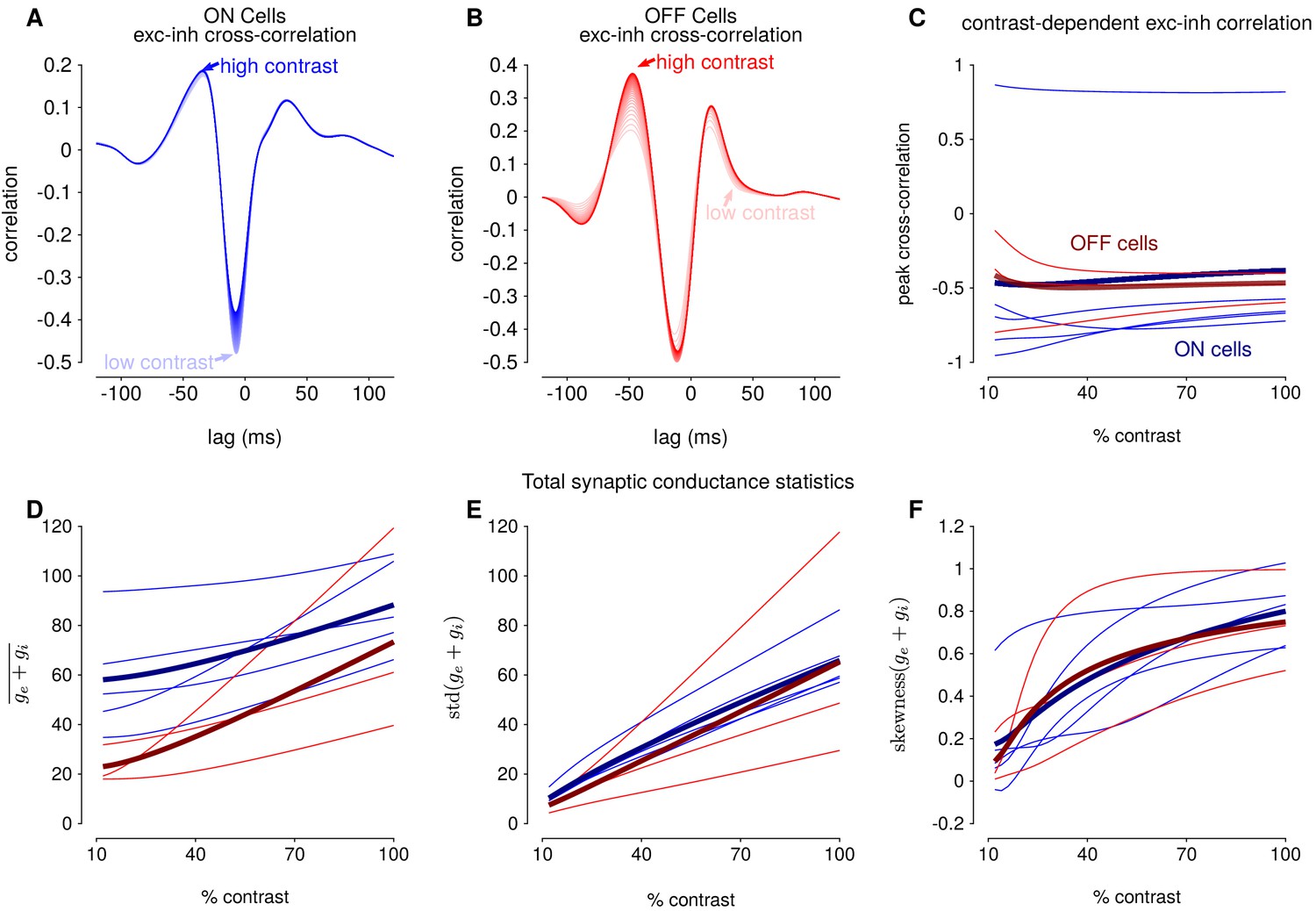
Correlation between the CBEM's excitation and inhibition depends on contrast.
(A) The average CBEM cross-correlation between excitation and inhibition for the 5 OFF cells fit to multi-contrast stimuli. The cross-correlations were computed from 12% (lightest trace) to 100% (darkest trace) contrast. (B) Same as A for the 3 ON cells. (C) The peak correlation between excitation and inhibition (maximum magnitude of the cross-correlation within 30 ms of 0 lag) as a function of contrast for all eight cells . The thick lines show the peak of the average cross-correlation for ON cells (blue) and OFF cells (red). The thin lines show the correlation for individual cells. (D) The mean total synaptic conductance in the CBEM fit ( averaged across time) as a function of contrast. Follows the same conventions as C. (E) The standard deviation of the total synaptic conductance as a function of contrast. (F) The skewness of the total synaptic conductance as a function of contrast. Unlike the mean and variance, the skewness in the CBEM fits begins to saturate with increased contrast.
Figure 10
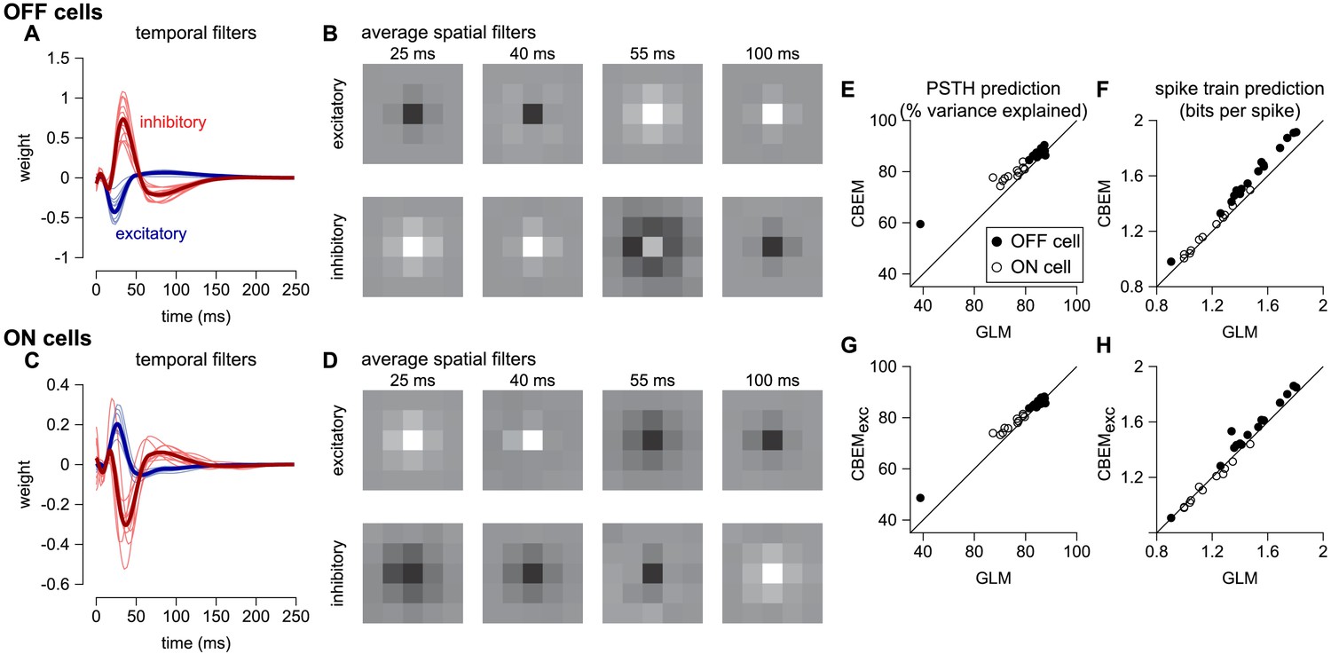
CBEM fits to a population of 27 RGCs.
(A) Temporal profile of the excitatory (blue) and inhibitory (red) at the center pixel of the receptive field for 16 OFF parasol cells. The thick lines show the mean. (B) The mean spatial profiles of the excitatory (top) and inhibitory (bottom) linear filters at four different time points for the OFF parasol cells. (C,D) same as A,B for 11 ON parasol cells. (E) Spike rate prediction performance of the CBEM compared to the GLM for the population of 27 cells for 8 s test stimulus. The true rate (black) was estimated using 600 repeat trials. (F) Log-likelihood of the CBEM compared to the GLM computed on a 5-min test stimulus. (G) Spike rate prediction performance of the CBEMexc compared to the GLM. (H) Log-likelihood of the CBEMexc compared to the GLM.
Figure 11
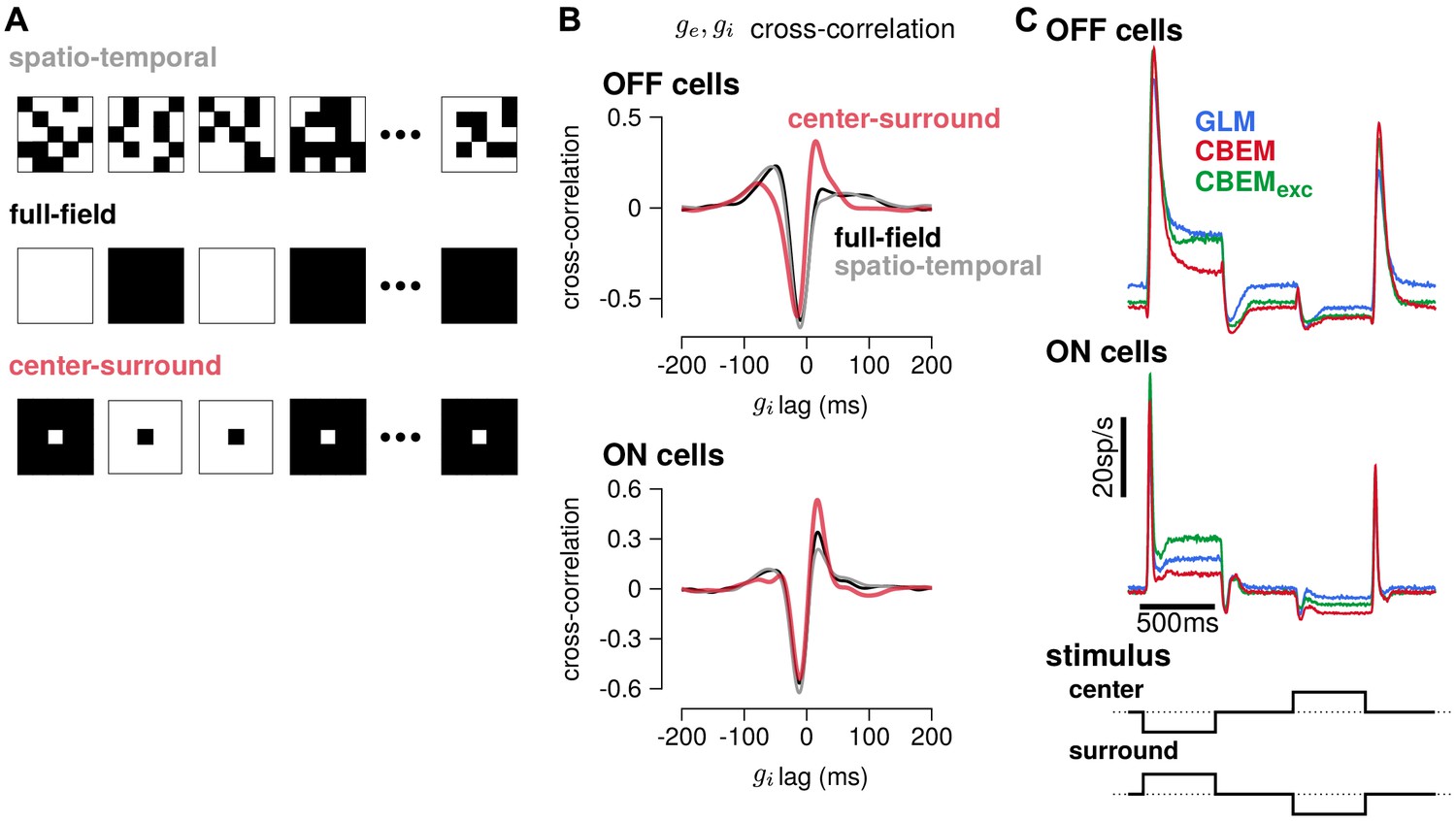
Predicted responses to spatially structured stimuli.
(A) Example sequences of 5 × 5 pixel frames of three different types of spatiotemporal noise stimuli used to probe the CBEM. The spatio-temporal stimulus was the same binary noise stimulus used to fit the cells. The full-field stimulus consisted of binary noise at the same contrast and frame rate as the original spatio-temporal stimulus. In the opposing center-surround condition, the center pixel was of opposite contrasts to the surround pixels and the sign of the center pixel was selected randomly on each frame. (B) The mean cross-correlation of the CBEM predicted excitatory and inhibitory conductances for the OFF cells (top) and ON cells (bottom) in response to full-field noise (black), spatio-temporal noise (grey), and opposing center-surround noise (red). The strong negative component showed that is delayed and oppositely tuned compared to . (C) Average firing rate of the GLM (blue), CBEM (red), and CBEMexc (green) fits to 16 OFF cells (top) and 11 ON cells (middle) in response to opposing center-surround contrasts steps (bottom).
Additional files
Download links
A two-part list of links to download the article, or parts of the article, in various formats.
Downloads (link to download the article as PDF)
Open citations (links to open the citations from this article in various online reference manager services)
Cite this article (links to download the citations from this article in formats compatible with various reference manager tools)
Inferring synaptic inputs from spikes with a conductance-based neural encoding model
eLife 8:e47012.
https://doi.org/10.7554/eLife.47012


