During hippocampal inactivation, grid cells maintain synchrony, even when the grid pattern is lost
- Technion – Israel Institute of Technology, Israel
- Bar Ilan University, Israel
- Norwegian University of Science and Technology, Norway
Figures
Figure 1
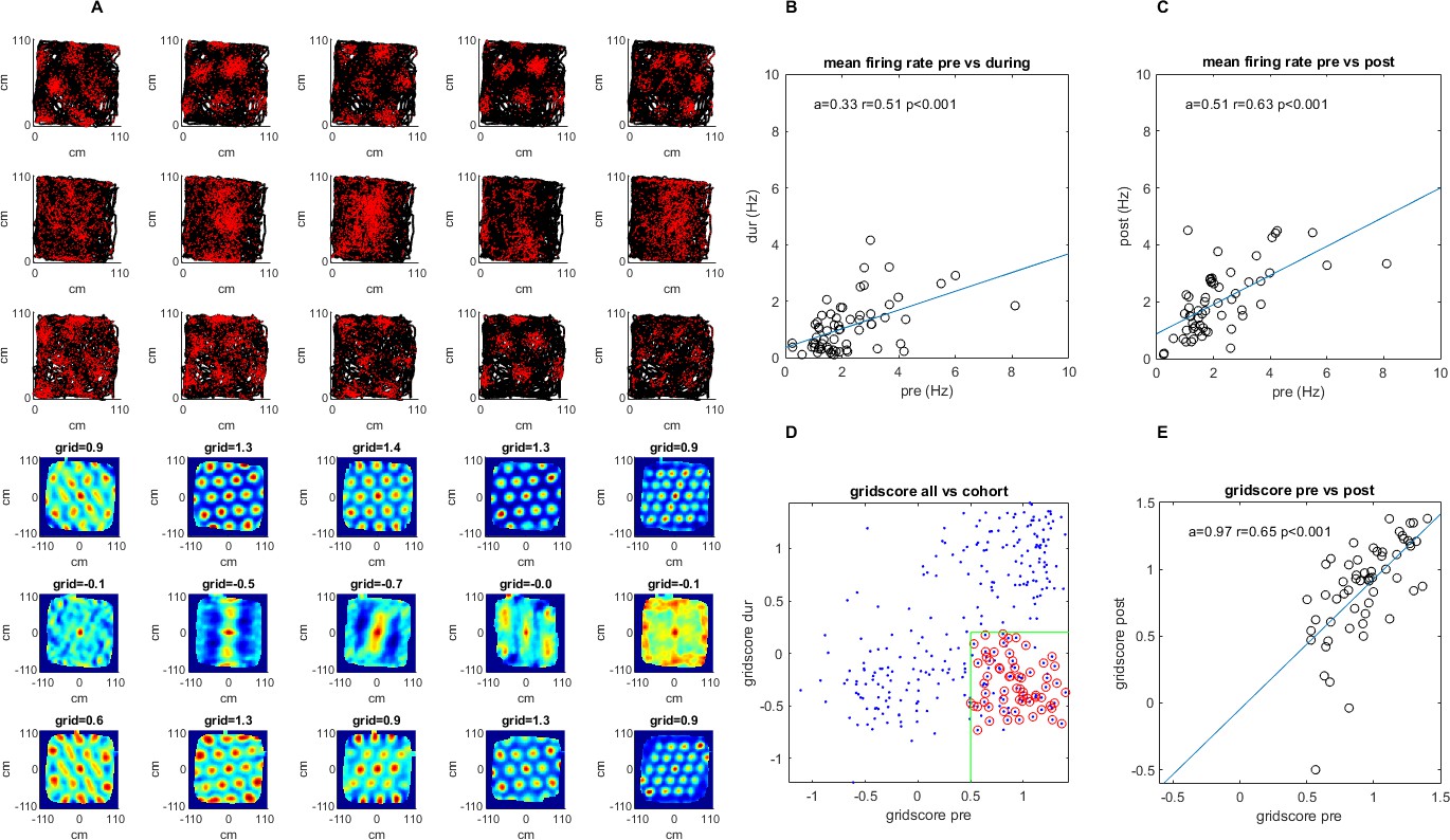
A survey of the grid cell population included in the study.
Recordings were made pre-, during, and post-injection of muscimol to the hippocampus. (A) A sample group of 5 simultaneously recorded grid cells, one cell per column. The first three plots in each column show the location of a single cell firing (red) along the rat’s trajectory (black) in a square arena pre-, during, and post-hippocampal inactivation, respectively. The last three plots in each column show the autocorrelation of the firing rate map and the grid score of that session pre-, during, and post inactivation. (B) The mean firing rate for the 63 grid cells included in the study pre- vs. during inactivation. (C) Same as (B) but for pre- vs. post-inactivation. (D) The grid score of all cells in the dataset vs. those included in the study. Red circles show the cells from the total population that were ultimately included in the study meeting the minimum and maximum grid score threshold pre- and during inactivation, respectively (green), as well as the additional criteria specified in the Materials and methods section (note that cells whose grid scores could not be calculated were set to 0). (E) Grid score pre- and post-inactivation of the cells included in the study.
Figure 2

Temporal and spatial cross correlations of simultaneously recorded grid cells pre- and during hippocampal inactivation.
(A) An example of a pair of simultaneously recorded grid cells (columns 1, 2); the location of the cell firing (red) plotted over the rat’s trajectory (black) in a square arena. Columns 3 and 4 show the temporal and spatial cross correlation of the firing rate maps of the cells, respectively. Rows show the same analysis pre- and during inactivation. (B) The temporal and spatial cross correlations of cell pairs of an entire group of simultaneously recorded grid cells (one pair per column). Rows 1, 2 show temporal correlations pre- and during inactivation; rows 3, 4 show the same for spatial cross correlations.
Figure 3 with 6 supplements
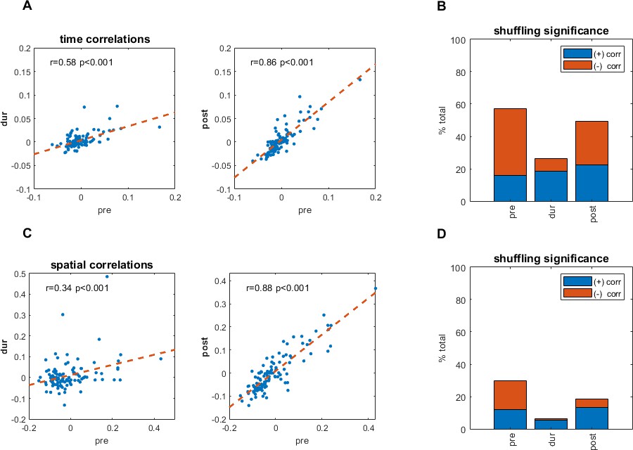
Temporal and spatial correlations pre- and during inactivation, for simultaneously recorded cell pairs.
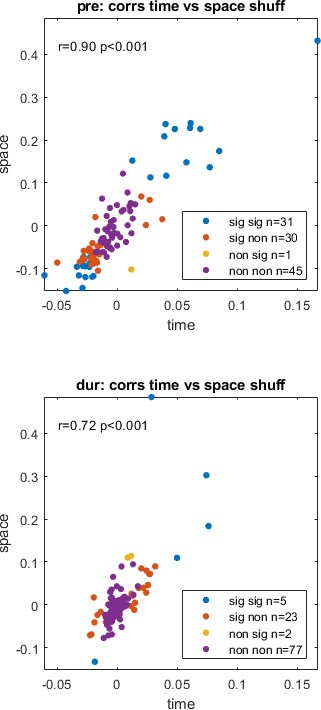
(A) Temporal cross correlations pre- and during inactivation, and pre- and post-inactivation, with correlation value (r), and corresponding p-value. (B) Proportions of significant temporal correlations, according to shuffling measures, pre-, during, and post-inactivation, including the sign (positive, negative) of the correlation value. (C) Same as (A) but for spatial correlations of the firing pattern in the arena at [0,0]. (D) Same as (B) but for spatial correlations of the firing pattern in the arena at [0,0].
Figure 3—figure supplement 1
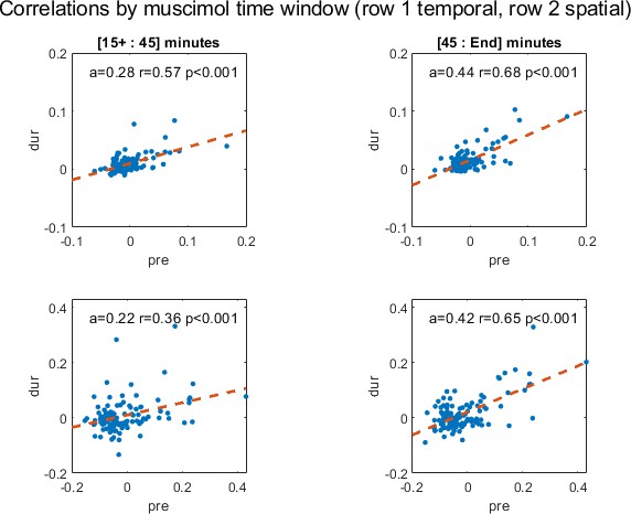
Temporal correlations pre-inactivation plotted against the recording period during inactivation used in this analysis for cell pairs in cohort; all recordings after muscimol injections are from 15 to 45 minutes (top left) and all remaining recordings are from 45 minutes (top right) of the muscimol recording session.
Slope of the regression line (a), correlation coefficient (r) and p-value (p) are shown. The second row depicts the same plots for spatial correlations. Because recordings had different starting and ending times, [15+, end] are used to signify the start and end of the recording time; on average, recordings started 16 minutes after and ended 115 minutes after muscimol injection into the hippocampus.
Figure 3—figure supplement 2
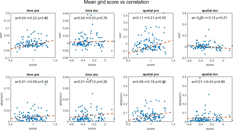
Temporal and spatial correlations for cell pairs in cohort pre- and during inactivation plotted against their average grid score, including slope of the regression line (a), correlation coefficient (r) and p-value (p).
The second row shows the same plots for absolute correlation values.
Figure 3—figure supplement 3
Temporal correlations plotted against spatial correlations for the cell pairs in our cohort, highlighted by significance, pre- (top) and during inactivation (bottom) with correlation coefficient (r) and p-value (p).
The legend shows temporal significance followed by spatial significance, with either being significant (sig) or non-significant (non), that is ‘non sig’ implies the temporal correlation was non-significant and the spatial correlation was significant.
Figure 3—figure supplement 4

Drift rate plots for different time windows for all pairs in cohort.
For each pair of cells: each spike’s location was subtracted from that of all spikes from the second cell for a given time (t) window [-t, t]. These location differences were added to matrix of bins where the index [i,j] was the difference in cm for the spikes’ x and y locations. This matrix was divided element-wise by a matrix of homologous construction where each bin represented the amount of time the animal spent for that x,y difference with respect to each spike, thus producing an aggregate 'rate' matrix per cell pair. These 2D difference rate matrices are shown in (A) for a one second time window pre- and during inactivation for three cell pairs. (B) shows these 2D matrices correlated to each other, pre- vs. during inactivation on the y axis, and pre- vs. post-inactivation along the x axis, with slope of trendline (a), correlation coefficient (r) and p-value (p). For a more thorough description of this analysis see Materials and methods.
Figure 3—figure supplement 5
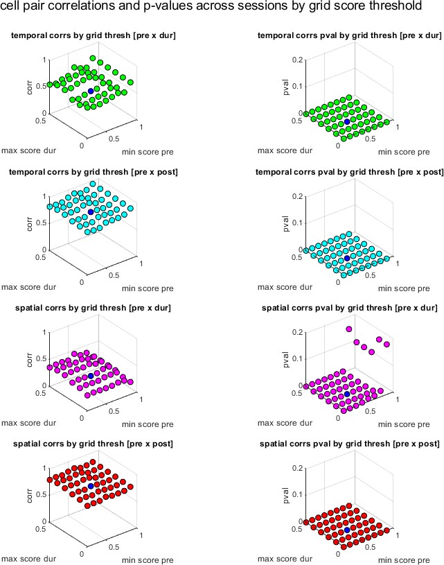
Cell pair correlations between sessions and p-values as a function of the grid score thresholds used in cell pair selections.
In the first column, x and y axis show the pre- and during inactivation grid score thresholds used to select simultaneously recorded cell pairs, the z axis shows the vector of those cell pair correlations (temporal and spatial) correlated against the same set of pairs for a different session (pre- vs. during inactivation, and pre- vs. post-inactivation). The column on the right shows the corresponding p-value for each of those correlations. Note that blue is the actual value of thresholds used in the paper.
Figure 3—figure supplement 6
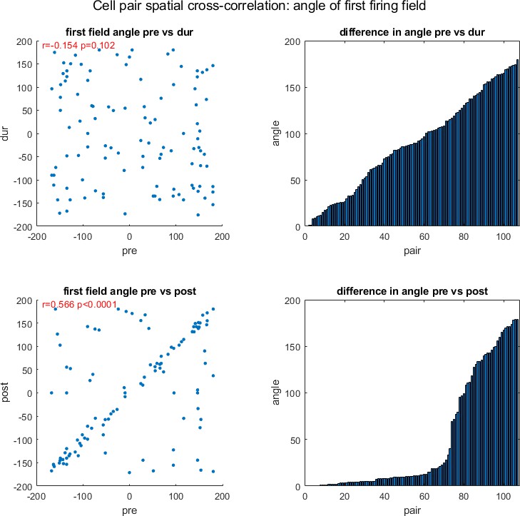
Examining the angle of firing fields for cross-correlated cells.
Here the spatial firing rate maps of two cells are spatially cross correlated and the angle between the closest firing field to the center-most firing field is calculated. The first column shows scatter plots of the angle pre- and during inactivation, and pre- and post-inactivation, including correlation using circular statistics (r) and corresponding p-value (p). The second column shows the difference in angle between two sessions for each cell pair, pre- vs. during inactivation, and pre- vs. post-inactivation, y axis shows the angle difference, x axis the pair number (note the difference angles are sorted in ascending order, consequently the x axis only represents the pair number with respect to its own plot, not both). All angles are in degrees.
Figure 4 with 2 supplements
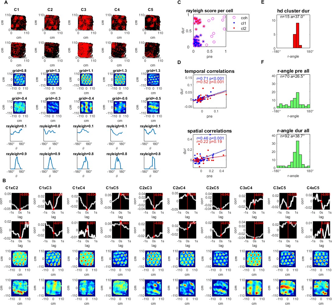
Simultaneously recorded grid cells that became head directional during hippocampal inactivation.
(A) A sample group of 5 simultaneously recorded grid cells, one cell per column. The first two plots in each column show the location of a single cell firing (red) along the rat’s trajectory (black) in a square arena pre- and during hippocampal inactivation. Next, two plots show the autocorrelation of the firing rate map and the associated grid score pre- and during inactivation. The last two plots in the column show the firing rate by head direction with an associated Rayleigh score, pre- and during inactivation. (B) Temporal and spatial cross correlations for each cell pair of the group, pre- and during inactivation by column. (C) Rayleigh scores pre- and during inactivation for all cells in the cohort (magenta circles) clustered by low head directionality (Rayleigh score <0.4 pre- and during inactivation, blue) and high head directionality (Rayleigh score <0.4 pre- and >0.4 during inactivation, red) (D) Temporal and spatial correlations (at 0,0) pre- and during inactivation grouped by head directionality clusters defined in (C), with the trendline slope (a) correlation coefficient (r), and corresponding p-value (p). (E) Histogram of Rayleigh angles for the cells in the HD cluster (red cluster in panels C and D) during inactivation (angles pre-inactivation are not shown since these cells had low Rayleigh scores for that period). (F) Rayleigh angles for all cells in population with Rayleigh score >0.4 pre-, and during inactivation.
Figure 4—figure supplement 1
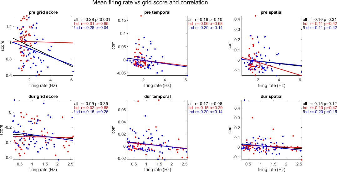
The mean firing rate of cohort cell pairs plotted against their mean grid score, temporal and spatial correlations, pre- and during inactivation (rows 1 and 2, respectively), grouped by cells with head direction selectivity during inactivation (Rayleigh score <0.4 pre- and >0.4 during inactivation, red), and without head direction selectivity during inactivation (Rayleigh score <0.4 pre- during inactivation, blue), and all pairs in cohort (black), with correlation coefficient (r) and p-value (p).
https://doi.org/10.7554/eLife.47147.012
Figure 4—figure supplement 2
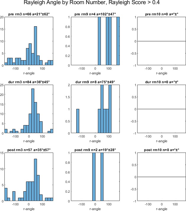
Rayleigh angles for all head direction cells in population by room number (rm#), for cells with Rayleigh score greater than 0.4, pre-, during and post- inactivation (rows 1, 2, 3, respectively), with number of cells (n) and average (a) +- standard deviation angle.
Note that most head direction cells were recorded in room 3, and no head direction cells were recorded in room 10.
Additional files
-
Transparent reporting form
- https://doi.org/10.7554/eLife.47147.014
Download links
A two-part list of links to download the article, or parts of the article, in various formats.
Downloads (link to download the article as PDF)
Open citations (links to open the citations from this article in various online reference manager services)
Cite this article (links to download the citations from this article in formats compatible with various reference manager tools)
During hippocampal inactivation, grid cells maintain synchrony, even when the grid pattern is lost
eLife 8:e47147.
https://doi.org/10.7554/eLife.47147


