Brian 2, an intuitive and efficient neural simulator
- Sorbonne Université, INSERM, CNRS, Institut de la Vision, France
- Imperial College London, United Kingdom
Figures
Figure 1
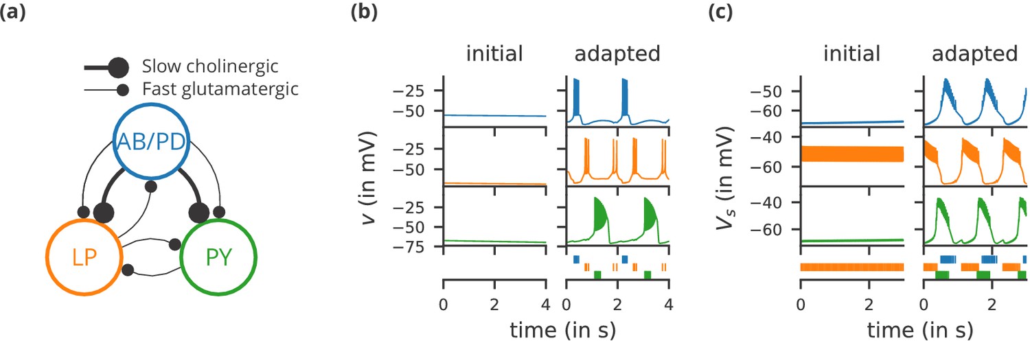
Case study 1: A model of the pyloric network of the crustacean stomatogastric ganglion, inspired by several modelling papers on this subject (Golowasch et al., 1999; Prinz et al., 2004; Prinz, 2006; O'Leary et al., 2014).
(a) Schematic of the modelled circuit (after Prinz et al., 2004). The pacemaker kernel is modelled by a single neuron representing both anterior burster and pyloric dilator neurons (AB/PD, blue). There are two types of follower neurons, lateral pyloric (LP, orange), and pyloric (PY, green). Neurons are connected via slow cholinergic (thick lines) and fast glutamatergic (thin lines) synapses. (b) Activity of the simulated neurons. Membrane potential is plotted over time for the neurons in (a), using the same colour code. The bottom row shows their spiking activity in a raster plot, with spikes defined as excursions of the membrane potential over −20 mV. In the left column (‘initial’), activity is shown for 4 s after an initial settling time of 2.5 s. The right column (‘adapted’) shows the activity with fully adapted conductances (see text for details) after an additional time of 49 s. (c) Activity of the simulated neurons of a biologically detailed version of the circuit shown in (a), following (Golowasch et al., 1999). All conventions as in (b), except for showing 3 s of activity after a settling time of 0.5 s (‘initial’), and after an additional time of 24 s (‘adapted’). Also note that the biologically detailed model consists of two coupled compartments, but only the membrane potential of the somatic compartment () is shown here.
Figure 2 with 1 supplement
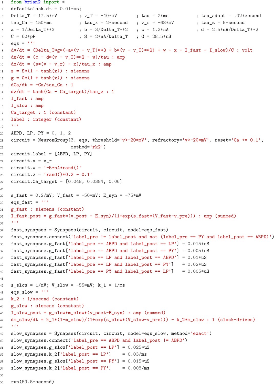
Case study 1: A model of the pyloric network of the crustacean stomatogastric ganglion.
Simulation code for the model shown in Figure 1a, producing the circuit activity shown in Figure 1b.
Figure 2—figure supplement 1
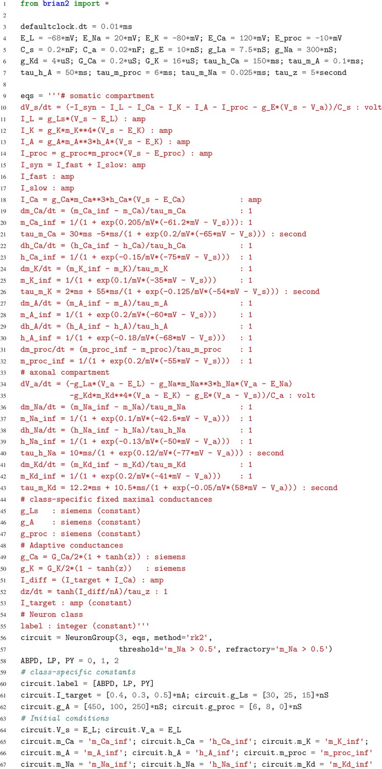
Simulation code for the more biologically detailed model of the circuit shown in Figure 1a, producing the circuit activity shown in Figure 1c.
Simulation code for the more biologically detailed model of the circuit shown in Figure 1a (based on Golowasch et al., 1999). The code for the synaptic model and connections is identical to the code shown in Figure 2, except for acting on instead of in the target cell.
Figure 3
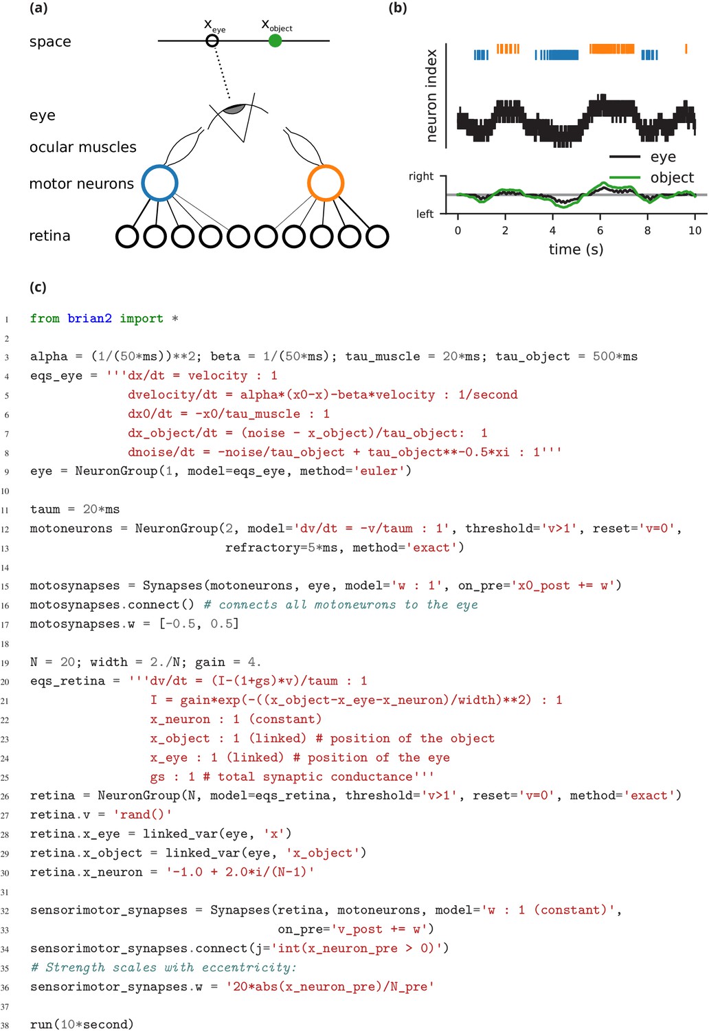
Case study 2: Smooth pursuit eye movements.
(a) Schematics of the model. An object (green) moves along a line and activates retinal neurons (bottom row; black) that are sensitive to the relative position of the object to the eye. Retinal neurons activate two motor neurons with weights depending on the eccentricity of their preferred position in space. Motor neurons activate the ocular muscles responsible for turning the eye. (b) Top: Simulated activity of the sensory neurons (black), and the left (blue) and right (orange) motor neurons. Bottom: Position of the eye (black) and the stimulus (green). (c) Simulation code.
Figure 4

Case study 3: Using bisection to find a neuron’s voltage threshold.
(a) Schematic of the bisection algorithm for finding a neuron’s voltage threshold. The algorithm is applied in parallel for different values of sodium density. (b) Top: Refinement of the voltage threshold estimate over iterations for three sodium densities (blue: 23.5 mS cm−2, orange: 57.5 mS cm−2, green: 91.5 mS cm−2); Bottom: Voltage threshold estimation as a function of sodium density.
Figure 5
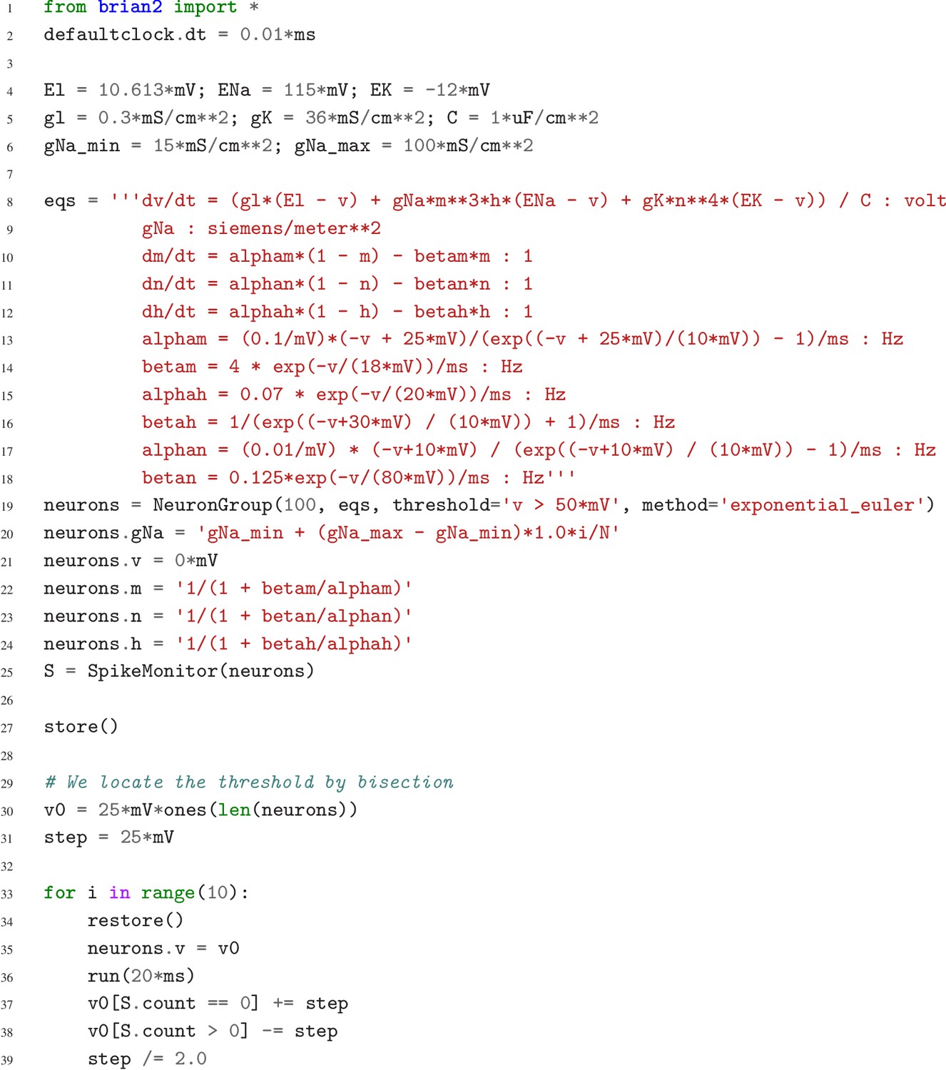
Case study 3: Simulation code to find a neuron’s voltage threshold, implementing the bisection algorithm detailed in Figure 4a.
The code simulates 100 unconnected neurons with sodium densities between 15 mS cm−2 and 100 mS cm−2, following the model of Hodgkin and Huxley (1952). Results from these simulations are shown in Figure 4b.
Figure 6
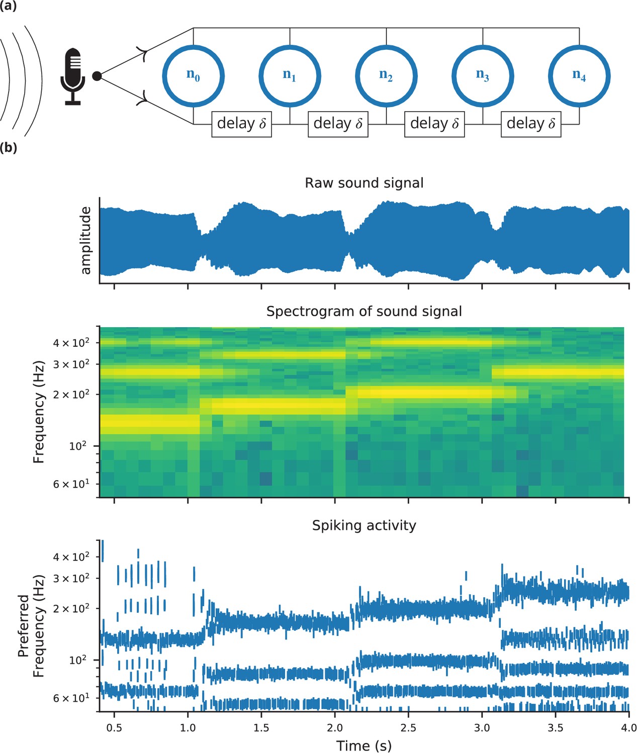
Case study 4: Neural pitch processing with real-time input.
(a) Model schematic: Audio input is converted into spikes and fed into a population of coincidence-detection neurons via two pathways, one instantaneous, that is without any delay (top), and one with incremental delays (bottom). Each neuron therefore receives the spikes resulting from the audio signal twice, with different temporal shifts between the two. The inverse of this shift determines the preferred frequency of the neuron. (b) Simulation results for a sample run of the simulation code in Figure 7. Top: Raw sound input (a rising sequence of tones – C, E, G, C – played on a synthesised flute). Middle: Spectrogram of the sound input. Bottom: Raster plot of the spiking response of receiving neurons (group neurons in the code), ordered by their preferred frequency.
Figure 7
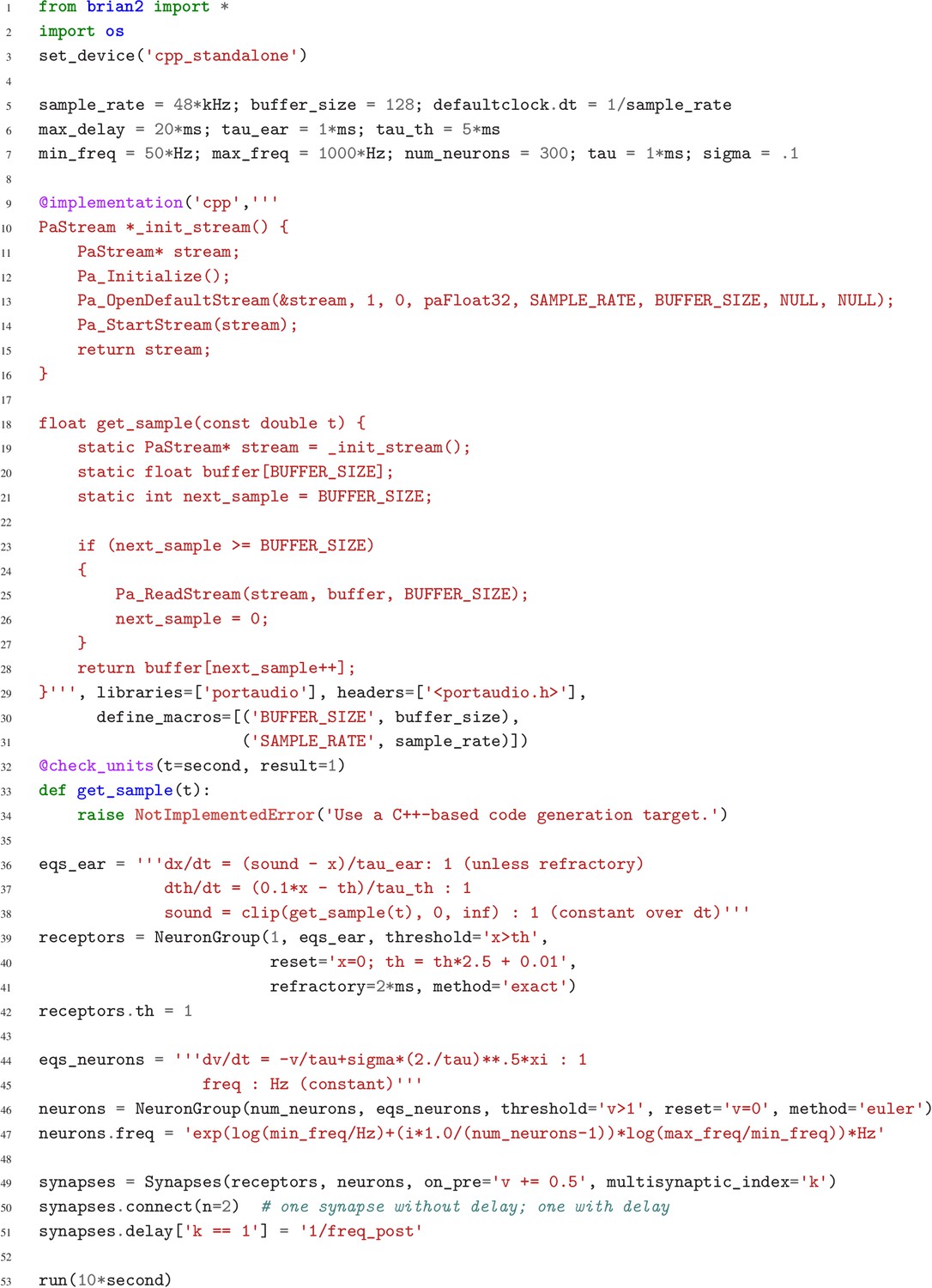
Case study 4: Simulation code for the model shown in Figure 6a.
The sound input is acquired in real time from a microphone, using user-provided low-level code written in C that makes use of an Open Source library for audio input (Bencina and Burk, 1999).
Figure 8

Benchmark of the simulation time for the CUBA network (Vogels and Abbott, 2005; Brette et al., 2007), a sparsely connected network of leaky-integrate and fire network with synapses modelled as exponentially decaying currents.
Synaptic connections are random, with each neuron receiving on average 80 synaptic inputs and weights set to ensure ongoing asynchronous activity in the network. The simulations use exact integration, but spike spike times are aligned to the simulation grid of 0.1 ms. Simulations are shown for a homogeneous population (left), where the membrane time constant, as well as the excitatory and inhibitory time constant, are the same for all neurons. In the heterogeneous population (right), these constants are different for each neuron, randomly set between 90% and 110% of the constant values used in the homogeneous population. Simulations were performed with NEST 2.16 (blue, Linssen et al., 2018, RRID:SCR_002963), NEURON 7.6 (orange; RRID:SCR_005393), Brian 1.4.4 (red), and Brian 2.2.2.1 (shades of green, Stimberg et al., 2019b, RRID:SCR_002998). Benchmarks were run under Python 2.7.16 on an Intel Core i9-7920X machine with 12 processor cores. For NEST and one of the Brian 2 simulations (light green), simulations made use of all processor cores by using 12 threads via the OpenMP framework. Brian 2 ‘runtime’ simulations execute C++ code via the weave library, while ‘standalone’ code executes an independent binary file compiled from C++ code (see Appendix 1 for details). Simulation times do not include the one-off times to prepare the simulation and generate synaptic connections as these will become a vanishing fraction of the total time for runs with longer simulated times. Simulations were run for a biological time of 10 s for small networks (8000 neurons or fewer) and for 1 s for large networks. The times plotted here are the best out of three repetitions. Note that Brian 1.4.4 does not support exact integration for a heterogeneous population and has therefore not been included for that benchmark.
-
Figure 8—source data 1
Benchmark results for the homogeneous network.
- https://doi.org/10.7554/eLife.47314.012
-
Figure 8—source data 2
Benchmark results for the heterogeneous network.
- https://doi.org/10.7554/eLife.47314.013
Appendix 2—figure 1
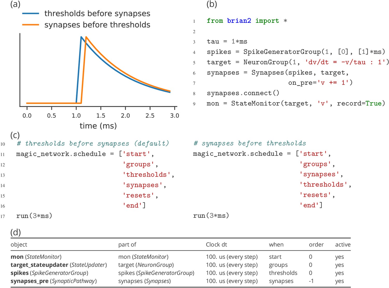
Demonstration of the effect of scheduling simulation elements.
(a) Timing of synaptic effects on the post-synaptic cell for the two simulation schedules defined in (c). (b) Basic simulation code for the simulation results shown in (a). (c) Definition of a simulation schedule where threshold crossings trigger spikes and – assuming the absence of synaptic delays – their effect is applied directly within the same simulation time step (left; see blue line in (a)), and a schedule where synaptic effects are applied in the time step following a threshold crossing (right; see orange line in (a)). (d) Summary of the scheduling of the simulation elements following the default schedule (left code in (c)), as provided by Brian’s scheduling_summary function. Note that for increased readibility, the objects from (b) have been explicitly named to match the variable names. Without this change, the code in (b) leads to the use of standard names for the objects (spikegeneratorgroup, neurongroup, synapses, and statemonitor).
Appendix 3—figure 1
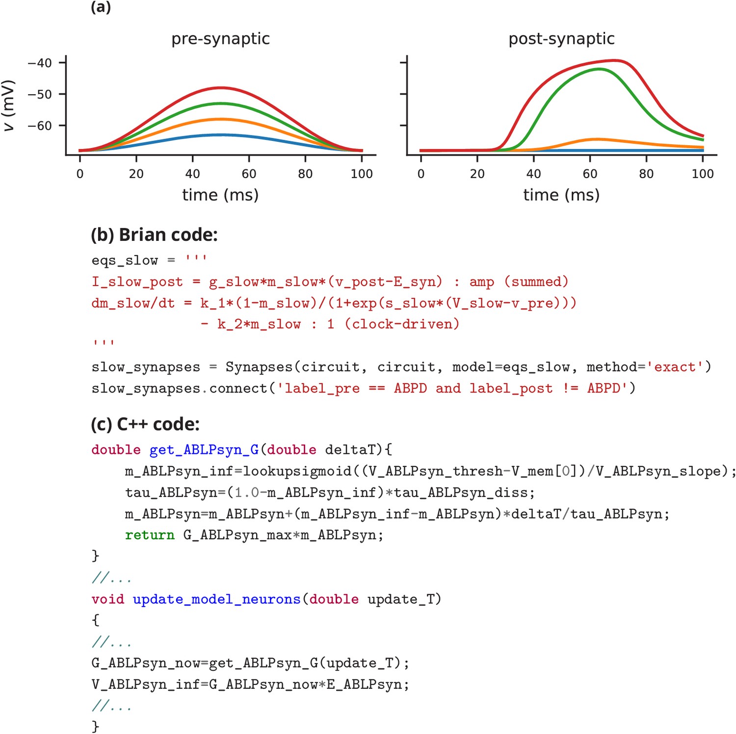
Graded synapse model.
(a) Demonstration of the effect of the graded synapse model used in case study 1 (Figure 1, Figure 2). On the left, the membrane potential excursion of a pre-synaptic neuron is modelled by a squared sinusoidal function of time with varying amplitudes from 5 mV to 20 mV. The plot on the right shows the post-synaptic membrane potential of a cell receiving graded synaptic input from the pre-synaptic cell via the graded synapse model from case study 1 (slow cholinergic synapse, cf. Golowasch et al., 1999). The post-synaptic cell is modelled here as a simple leaky integrator with a single synaptic input current. (b) Code excerpt showing the Brian 2 definition of the graded synapse model used in (a), taken from the code used in case study 1 (Figure 2). (c) Code excerpt defining a graded synapse model in C++ as part of 'The Pyloric Network Model Simulator' (http://www.biology.emory.edu/research/Prinz/database-sensors/; Günay and Prinz, 2010). The complete code is 3510 lines.
Appendix 3—figure 2
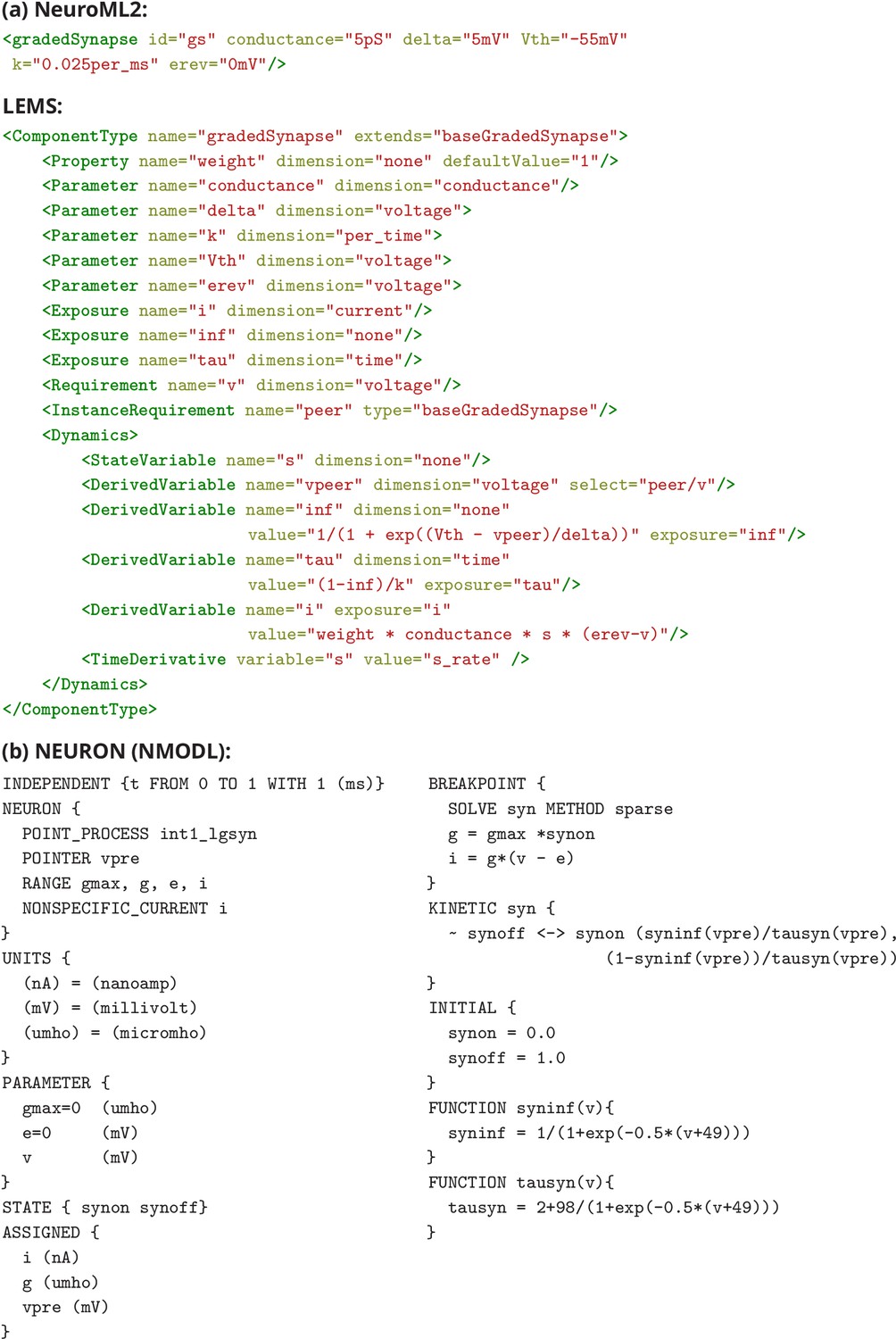
Graded synapse model (cont.).
(a) Definition of a graded synapse model in NeuroML2/LEMS. The graded synapse model as described in Prinz et al. (2004) has been added as a “core type” to the (not yet finalized) NeuroML2 standard and can therefore be accessed under the name gradedSynapse (top). It is fully defined via the LEMS definition partially reproduced here. (b) A definition of a graded synapse in the stomatogastric system, written in the NMODL language for the NEURON simulator. This model has been implemented in Nadim et al. (1998), see https://senselab.med.yale.edu/ModelDB/showmodel.cshtml?model=3511.
Appendix 4—figure 1
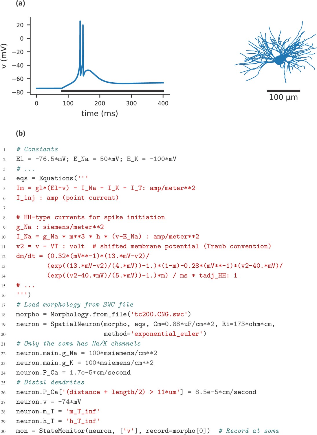
A multi-compartment model of a thalamic relay cell.
(a) Simulation of a thamalic relay cell with increased T-current in distal dendrites (partially reproducing Figure 9C from Destexhe et al. (1998). The plot shows the somatic membrane potential for a current injection of 75 pA during the period marked by the black line. The model consists of a total of 1291 compartments and is based on the morphology available on NeuroMorpho.Org (Ascoli et al., 2007) under the ID NMO_00881, displayed on the right. This morphology is a reconstruction of a cell in the rat’s ventrobasal complex, originally described in Huguenard and Prince (1992). (b) Selected lines from the simulation code implementing the model shown in (a), focussing on the differences to single-compartmental models (as shown in case studies 1–4).
Appendix 4—figure 2
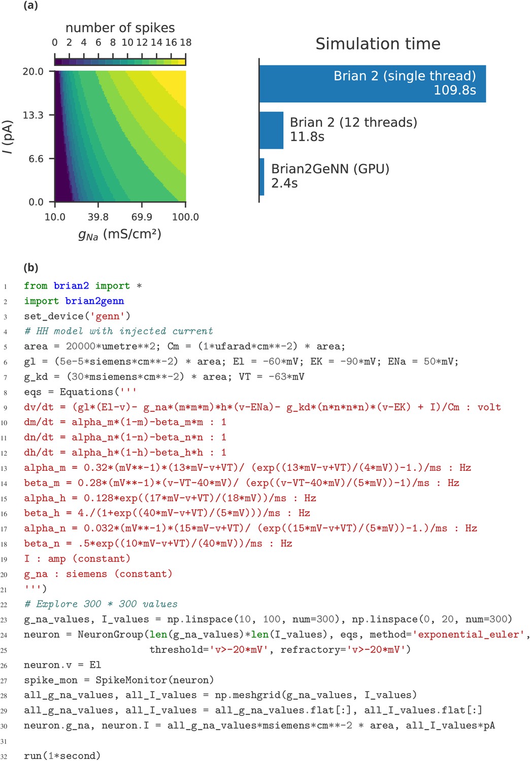
Parameter exploration over two parameters.
(a) In a single-compartment neuron model of the Hodgkin-Huxley type (following Traub and Miles, 1991), we record the number of spikes over 1 s while varying the strength of a constant input current , and the density of the sodium conductance for a total of 300 × 300 values. The bars on the right show the simulation time on the same machine used for Figure 8 when using Brian 2’s C++ standalone mode with a single thread (top), with 12 threads (middle), or when simulating it on a NVIDIA GeForce RTX 2080 Ti graphics card via the Brian2GeNN (Stimberg et al., 2018) interface to the GeNN (Yavuz et al., 2016) simulator (bottom). (b) Code for the simulation shown in (a), here configured to run on the GPU via the Brian2GeNN interface (l.2-3).
Additional files
-
Source code 1
Benchmarking code.
- https://doi.org/10.7554/eLife.47314.014
-
Transparent reporting form
- https://doi.org/10.7554/eLife.47314.015
Download links
A two-part list of links to download the article, or parts of the article, in various formats.
Downloads (link to download the article as PDF)
Open citations (links to open the citations from this article in various online reference manager services)
Cite this article (links to download the citations from this article in formats compatible with various reference manager tools)
Brian 2, an intuitive and efficient neural simulator
eLife 8:e47314.
https://doi.org/10.7554/eLife.47314


