Figures and data in A minimal self-organisation model of the Golgi apparatus

Figures
Tables
Additional files

14 figures, 3 tables and 2 additional files

Figures

Figure 1

Download asset Open asset

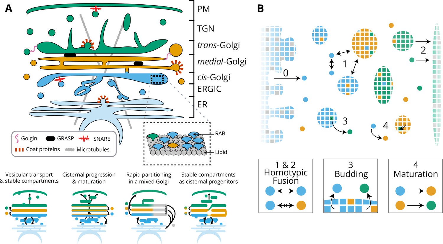
Model of golgi structure and transport.

(A) Top: classical representation of the structure of the Golgi, showing some of the important protein actors. The three main membrane identities are shown in different colors (*cis*: blue, *medial*: orange, *trans*: green): ER = Endoplasmic Reticulum, ERGIC = ER Golgi intermediate Compartment, TGN = Trans Golgi-Network, PM = Plasma Membrane. Bottom: Sketches of the four main models of Golgi transport (see text). (B) Our quantitative model of Golgi self-organisation. The left boundary is the ER, composed of a *cis*-membrane identity, and the right boundary is the TGN, composed of a *trans*-membrane identity. Golgi compartments self-organise *via* three stochastic mechanisms: Fusion: (1) All compartments can aggregate using homotypic fusion mechanisms: the fusion rate is higher between compartment of similar identities. (2) Each compartment can exit the system by fusing homotypically with the boundaries. Budding: (3) Each compartment larger than a vesicle can create a vesicle by losing a patch of membrane. Biochemical conversion: (4) Each patch of membrane undergoes a conversion from a *cis* to a *trans*-identity. New *cis*-vesicles (0) bud from the ER at a constant rate. In the sketch, the boundaries also contain neutral (gray) membrane species that dilute their identity (impact of this dilution in Appendix 7).

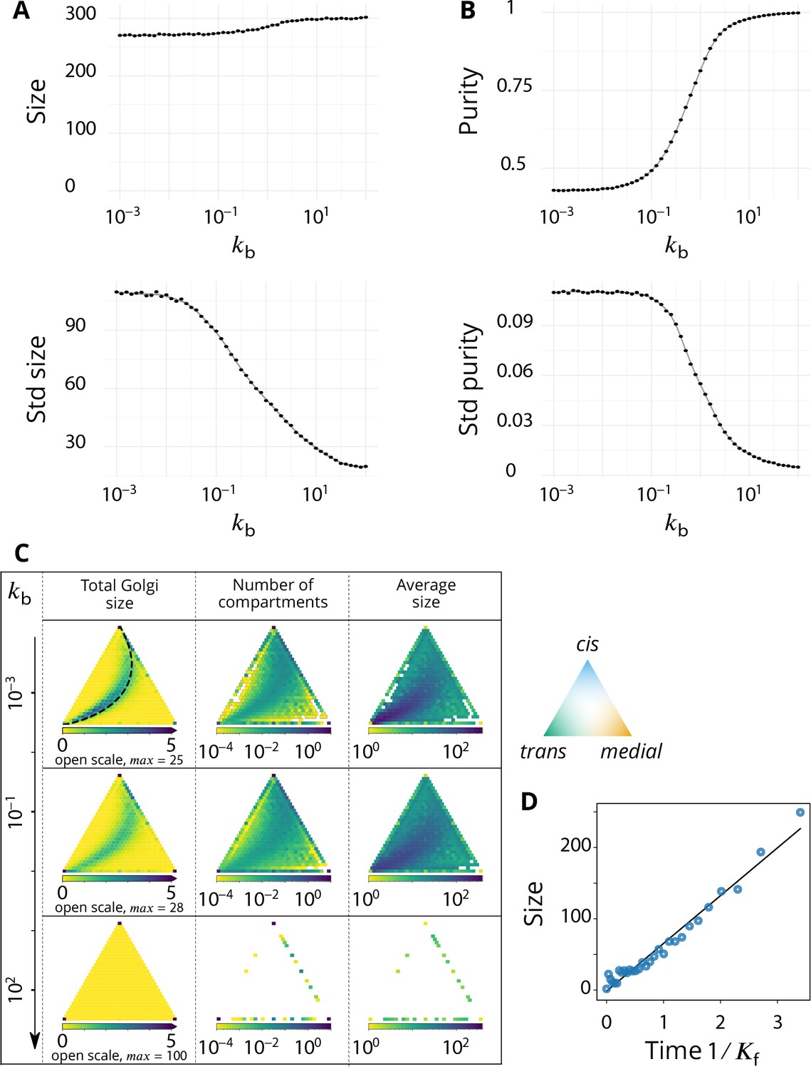
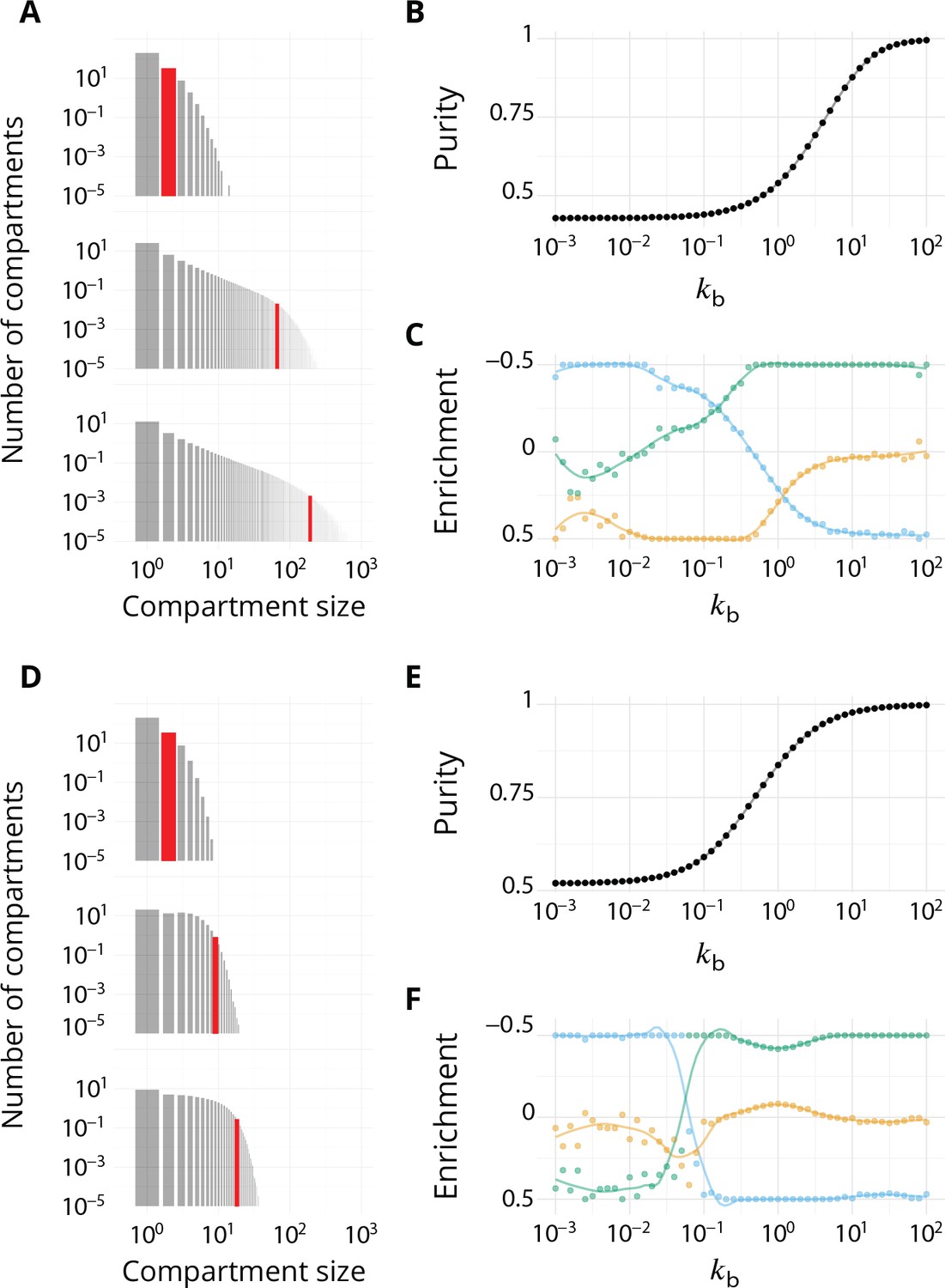
Figure 2

Download asset Open asset

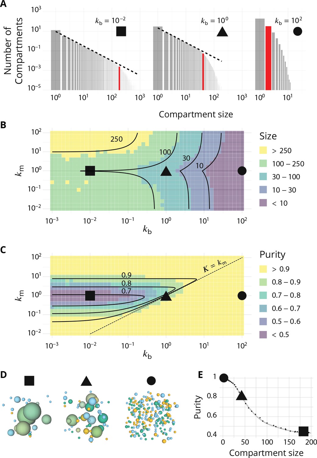
Steady-state of the self-organized model of Golgi apparatus.

(A) Size distribution of compartments for a biochemical conversion rate $k_{m} = 1$ and different values of the budding rate $k_{b}$ . The red bar shows the characteristic compartment size. (B) Phase diagram of the size of the compartments as the function of $k_{b}$ and $k_{m}$ . Black lines: theoretical prediction (Equations 4,6) (C) Phase diagram of the purity of the system as a function of $k_{b}$ and $k_{m}$ . Dashed line is $k_{m} = k_{b}$ , black lines are a theoretical prediction (see Appendix 3). (D) System snapshots for $k_{m} = 1$ showing the *mixed regime* (square - $k_{b} = 10^{- 2}$ ), the *sorted regime* (triangle - $k_{b} = 1$ ), and the *vesicular regime* (circle - $k_{b} = 10^{2}$ ) - see text. (E) Average compartment purity as a function of their average size, obtained by varying the budding rate $k_{b}$ for $k_{m} = 1$ (black dots: simulation results – gray line: guide for the eyes). For all panels, $α_{ER} = α_{TGN} = 1$ . See also Appendix 5 for further characterizations of the steady-state organisation, Appendix 7 for the role of composition of the exit compartment, and Appendix 8 for results with alternative budding and fusion kinetics.

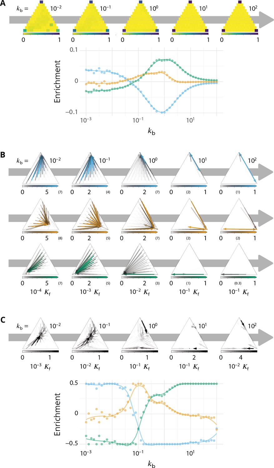
Figure 3

Download asset Open asset

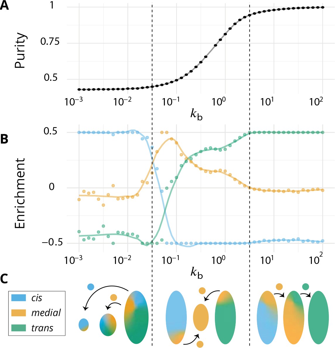
Directionality of vesicular transport, displayed varying the budding rate $k_{b}$ for a biochemical conversion rate $k_{m} = 1$ (equal amount of all species in the system).

(A) System purity as a function of the budding rate – a cut through the purity phase diagram shown Figure 2C. (B) Normalized enrichment in cis (blue), *medial* (orange) and *trans* (green) identities between the acceptor and donor compartments during vesicular exchange (solid lines are guides for the eyes). See Appendix 6 for non-normalized fluxes. (C) Sketches showing the direction of the dominant vesicular fluxes – consistent with data of A and B and data from Appendix 6—figure 1 – omitting less contributive transports. Before the purity transition (low values of $k_{b}$ - purity ~ 0.5) the vesicular flux is retrograde. After the transition (high values of $k_{b}$ - purity ~ 1) the vesicular flux is anterograde. Around the crossover ( $k_{b} \sim 0.1$ ), the vesicular flux is centripetal and oriented toward *medial*-compartments. The centripetal flux disappears if inter-compartments fusion is prohibited, see Appendix 8.

Figure 4

Download asset Open asset

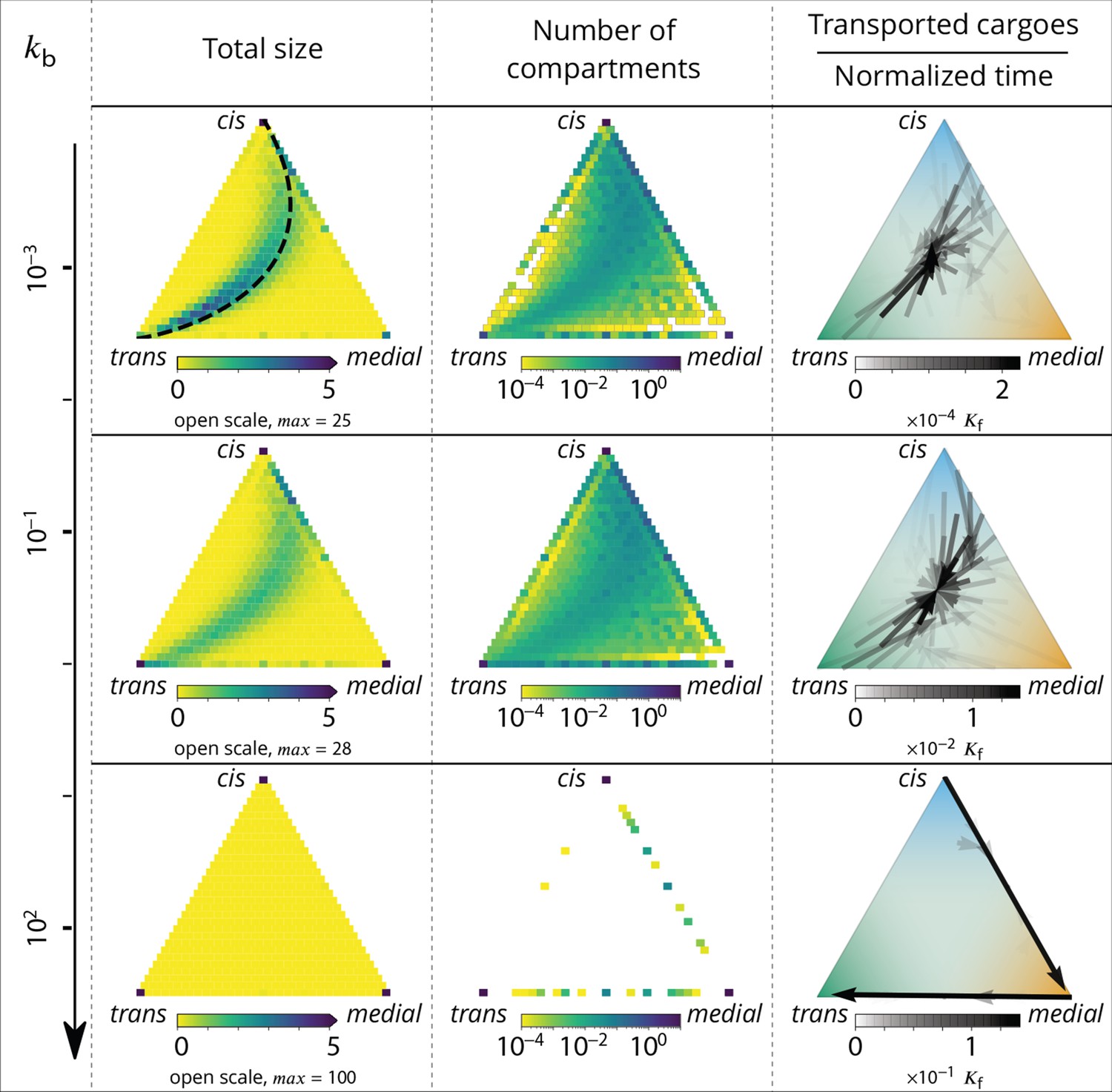
Relationship between the structure of the system and the vesicular fluxes.

Distribution of the total size of the system (truncated scale, maximum value in brackets) and number of compartments, and the vesicular flux between them, shown in a triangular composition space. Each point represents a given composition of compartments and the triangle vertices are compartments of pure *cis*, *medial* and *trans* identity. Arrows show the vesicular flux. The base of each arrow is the composition of the donor compartment and the tip is the average composition of receiving compartments (ignoring back fusion). The opacity of the arrows is proportional to the flux of transported cargo going through this path per unit time ( $1 / K_{f}$ ), normalized by the total number of cargo-proteins. The dashed line on the top-left triangle is the theoretical prediction given by Equation 9. See also Appendix 6 for further characterizations of the vesicular transport, and Appendix 8 to discuss the impact of other budding and fusion implementations on the vesicular fluxes.

Appendix 1—figure 1

Download asset Open asset

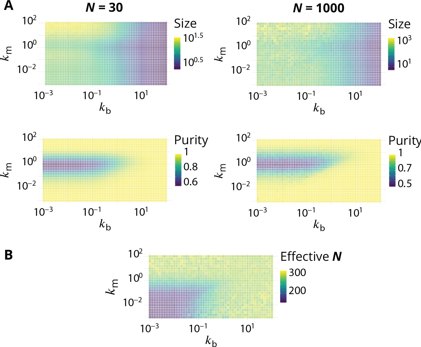
Link between the total size of the Golgi and its steady-state organisation.

(A) Size dependence of the steady-state organisation of the Golgi (to be compared with Figure 2 in the main text). We look at two different systems that only differ in term of the average total size $N$ , that equals 30 or 1000. Typical size of compartments and average system purity are shown as a function of $k_{m}$ and $k_{b}$ . In both cases $α = 1$ (see Appendix 1). (B) Average steady-state total size $N$ , as a function of $k_{m}$ and $k_{b}$ , for simulation in which the influx is set to have $N ≃ 300$ (using Equation 6).

Appendix 2—figure 1

Download asset Open asset

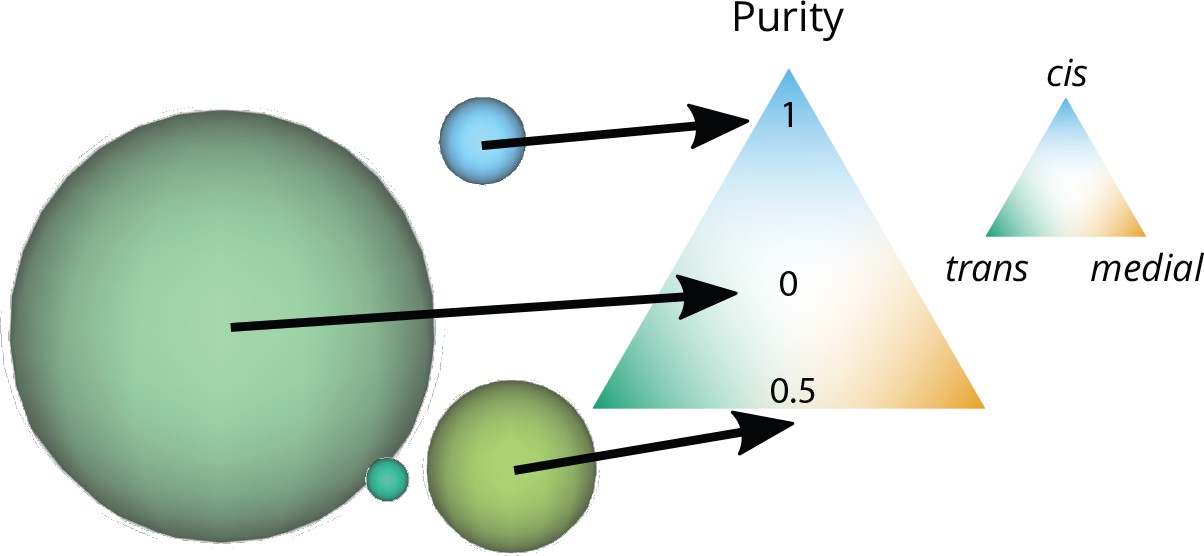
Graphical representation of the size and purity of compartments.

Each compartment is represented as a sphere with an area equal to the area of a vesicle (the smallest elements in this snapshot) times the number of vesicles that fused together to create the compartment. The color of the compartment reflects its composition, according to the color code on the triangular composition phase space: 100% *cis* at the top, *medial* at the bottom right, *trans* at the bottom left. The purity of each of these compartments is its distance from a perfectly mixed compartment at the center of the triangle (middle arrow). This distance is normalized so that it equals 1 for a perfectly pure compartment (bottom arrow).

Appendix 3—figure 1

Download asset Open asset

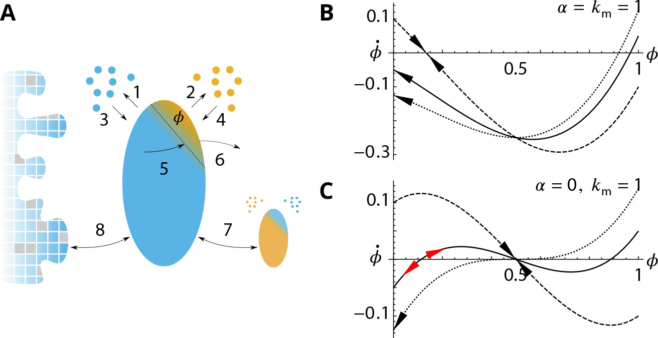
Analytical description of the *cis*-compartment purity.

Related to Figure 2 - main text. (A) Analytical model of the steady-state contamination by a *medial*-species (orange) of a *cis*-compartment (blue). The fraction occupied by the *medial*-species is named $ϕ$ . The eight events (1–8) impacting $ϕ$ are listed in the text. (**B-C**). Time variation $\dot{ϕ}$ as a function of $ϕ$ , with $k_{m} = 1$ and for different $k_{b}$ (0.9 dashed line, 1.05 solid line, and $1 + 1 / 8$ dotted line). $ϕ$ has a stable value when $\partial_{ϕ} \dot{ϕ} < 0$ and $\dot{ϕ} = 0$ or $\dot{ϕ} |_{ϕ = 0} < 0$ (black arrows). It is potentially unstable when $\partial_{ϕ} \dot{ϕ} > 0$ and ${\dot{ϕ}}_{ϕ \sim 0} = 0$ (red arrows). (B) For $α = 1 : k_{b} = 0.9$ (dashed) exhibits a stable fixed-point for $ϕ > 0$ but with $ϕ < 1 / 2$ as $α > 0; k_{b} = 1.05$ (solid) and $k_{b} = 1 + 1 / 8$ (dotted) exhibit a stable concentration for $ϕ = 0$ . (C) For $α = 0; k_{b} = 0.9$ (dashed) exhibits a stable fixed-point for $ϕ = 1 / 2; k_{b} = 1.05$ (solid) exhibits an unstable fixed-point near $ϕ = 0; k b = 1 + 1 / 8$ (dotted) does not display this unstable fixed-point as $k_{b} \geq k_{m} + 1 / 8$ (see text).

Appendix 4—figure 1

Download asset Open asset

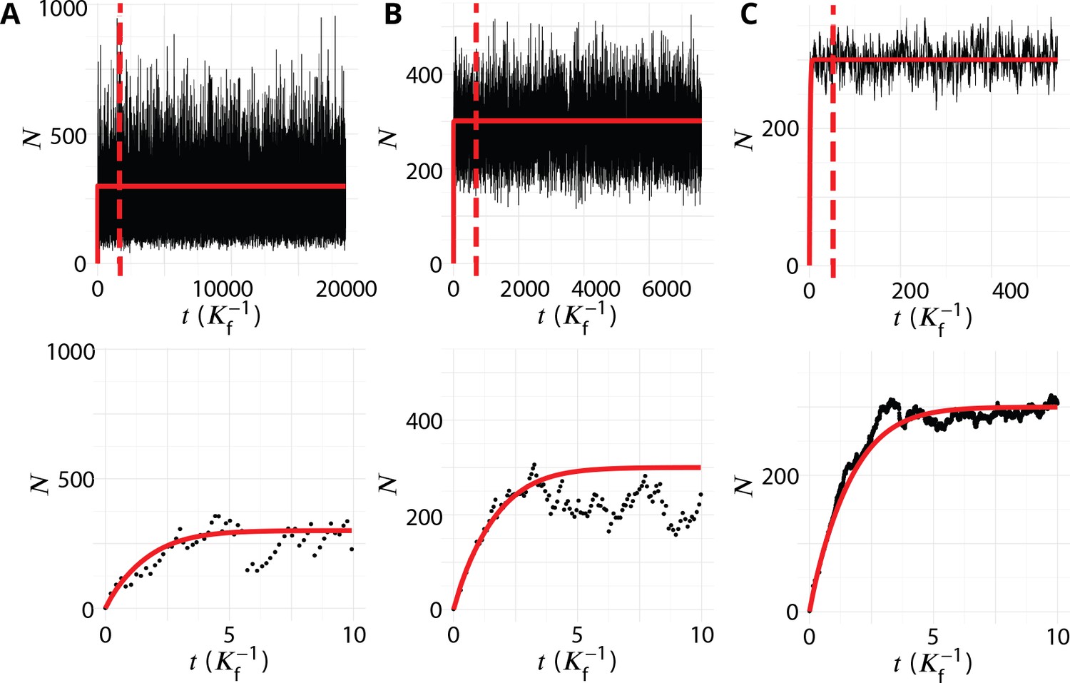
Transient regime towards the steady-state.

System’s size (total number of membrane patches in the system) as a function of time (in unit $1 / K_{f}$ ) for three different values of the budding rate (A: $k_{b} = 10^{- 2}$ , B: $k_{b} = 1$ , C: $k_{b} = 10^{2}$ ). The top row shows the full simulations, with a vertical dashed bar when the number of simulation steps reaches 10⁶. The steady-state data analysed and discussed in this paper are recorded after this time, and the full simulation typically lasted 10⁷ time-steps. The bottom row shows the evolution at early time (de-novo formation). The red lines are the analytical solution given by Appendix 4 Equation 3.

Appendix 4—figure 2

Download asset Open asset

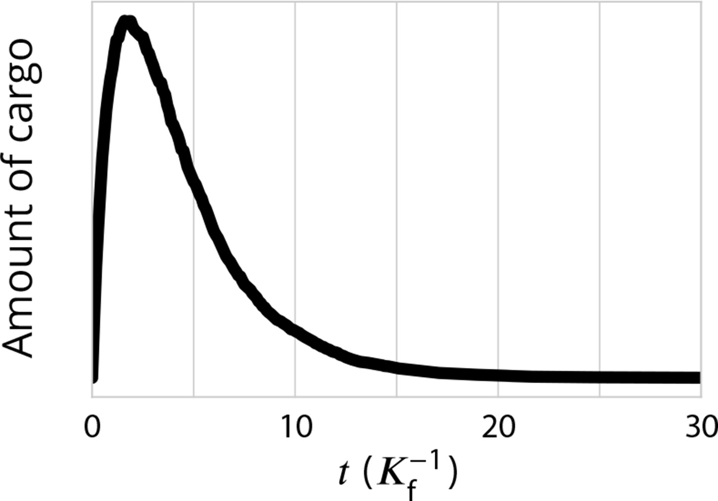
Exit kinetics of passive cargo.

Simulated amount of cargo in the Golgi following a pulse-chase like simulation in which 1000 cargo molecules are trapped in the ER and allowed to be packaged into ER exiting vesicles at $t = 0$ . This is expected to mimick the iFRAP experimental setup used in Patterson et al., 2008 and to the RUSH setup used in Boncompain et al., 2012. The decay of the amount of cargo is close to a single-time exponential decay, is agreement with experimental observations for transiting cargo (Figure 2i of Patterson et al., 2008 and Figure 3e in Boncompain et al., 2012). Parameters are $k_{b} = k_{m} = α = 1$ , corresponding to the ‘sorted regime’ (the triangle of Figure 2) which we expect to be the most reasonable for mammalian Golgi.

Appendix 5—figure 1

Download asset Open asset

Steady-state composition and fluctuation of compartments.

Related to Figure 2 - main text. (**A–B**) Characterization of the temporal fluctuations of the system as a function of the budding rate $k_{b}$ . (A) Average values of the system total size (top panel) and standard deviation of the size (bottom panel). (B) Average values of the system purity (top panel) and standard deviation of the purity (bottom panel). (C) Distribution of the total size, number of compartments and their average size, as a function of the composition of the compartments, shown in a triangle plot (see Appendix 2) for different values of the (normalized) budding rate $k_{b}$ . The average size for a given composition is calculated as the average size divided by the average number of compartments. Plots are shown for four different values of $k_{b}$ , with $k_{m} = α = 1$ . The dashed black line on the top, left panel (low $k_{b}$ regime) corresponds to the theoretical prediction of Equation 9. (D) The evolution of the compartment’s size as a function of time, in the low $k_{b} = 10^{- 3}$ limit, agrees with the linear prediction of Equation 7.

Appendix 6—figure 1

Download asset Open asset

Detailed characterizations of the vesicular transport.

Related to Figures 3–4 - main text. $α = k_{m} = 1$ for all panels. (A) Characterization of vesicle back-fusion (fusion of vesicles with the same compartment or with a compartment of comparable composition). Top panel: fraction of vesicular flux undergoing back-fusion, as a function of the composition of the budding compartments, for different values of the budding rate $k_{b}$ . Bottom panel: non-normalized enrichment in cis (blue), *medial* (orange) and *trans*-species (green) seen by a passive cargo, between a budding and the next fusion event, as a function of $k_{b}$ . (B) Vesicular fluxes of *cis* (blue), *medial* (orange) and *trans* (green) vesicles for different values of the budding rate $k_{b}$ . The base of each arrow gives the composition of the donor compartment and the tip gives the average composition of receiving compartments - ignoring back-fusion - as in Figure 4, main text. The opacity of the arrows represents the normalized number of cargo (divided by the total number of cargo in the system) transported per unit time (normalized by the fusion rate). (C) Net vesicular flux, excluding vesicle biochemical conversion, for different values of the budding rate $k_{b}$ . Top panel: vesicular flux is represented as a vector field as in Figure 4, main text. Bottom panel: vesicular flux is represented as the enrichment between the donor and the acceptor compartment, excluding back-fusion, as in Figure 3, main text.

Appendix 7—figure 1

Download asset Open asset

Impact of the composition of the boundaries of the system (ER and TGN) on the steady-state organisation.

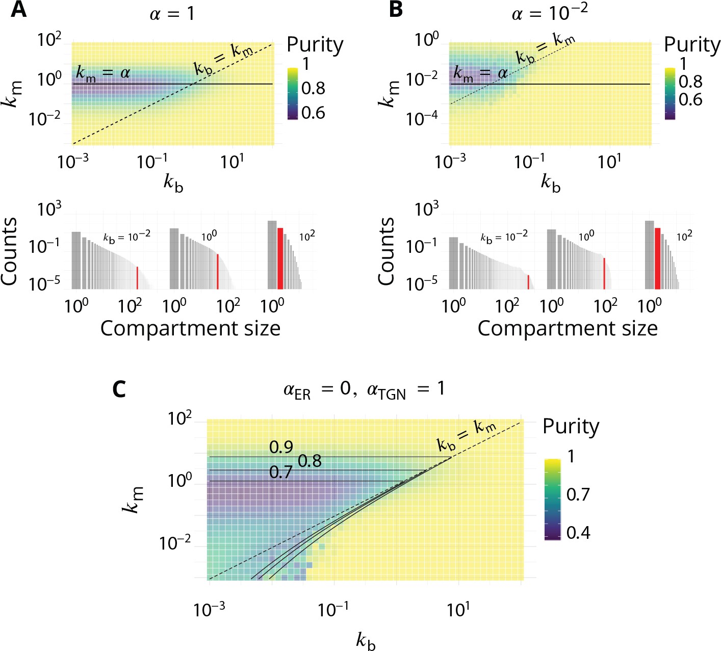
Related to Figure 2 - main text. (**A–B**). The fraction $α$ of active species driving homotypic fusion with the boundaries are identical for the ER and the TGN. A. $α = 1$ (same value as in the main text) B. $α = 10^{- 2}$ . For both cases, the top panel is the purity diagram as a function of the normalized biochemical conversion rate $k_{m}$ and budding rate $k_{b}$ . Dashed lines correspond to $k_{m} = k_{b}$ and solid lines to $k_{m} = α$ . For both cases, the bottom panel shows some examples of the size distribution for $k_{m} = α$ and different values of $k_{b}$ . (C) Purity diagram as a function of $k_{m}$ and $k_{b}$ when fusion with the ER is abolished: $α_{ER} = 0$ whereas $α_{TGN} = 1$ . Solid lines are the predictions of the analytical model developed in Appendix 3.

Appendix 8—figure 1

Download asset Open asset

Impact of different budding and fusion kernels on the system's organisation and vesicular transport.

Related to Figures 2–4 - main text. $k_{m} = α = 1$ . (**A–C**) Linear budding scheme. (**D–F**) Inter-compartment fusion is prohibited. (A and D) Size distribution of compartment for $k_{b}$ equals 10² (top), 1 (middle) and 10² (bottom). (B and E) Steady-state purity as a function of $k_{b}$ . (C and F) Enrichments in cis (blue), *medial* (orange) and *trans*-species (green) during vesicular transport (details of computations of this enrichment presented in Appendix 2) as a function of $k_{b}$ .

Appendix 9—figure 1

Download asset Open asset

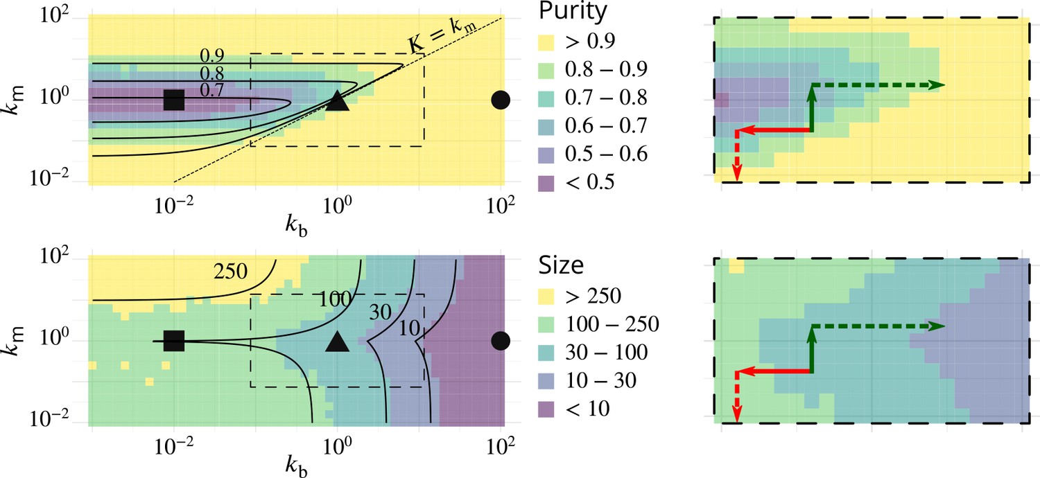
Possible experimental strategies to test the predicted correlation between size and purity of Golgi cisternae.

The left column reproduces Figure 2B–C, showing the phase diagrams for the purity (top) and size (bottom) of Golgi cisternae upon varying the ratio of budding to fusion rates $k_{b}$ and the ratio of biochemical conversion to fusion rate $k_{m}$ . The right column shows a zoom of the dashed square area, showing the observed result of physiological perturbations of cisternae purity and size (solid arrows) and prediction for combined perturbations (dashed arrows). Red arrow: observed result of a decrease of the budding rate $k_{b}$ by impairing COP I (Papanikou et al., 2015). Dashed red arrow: prediction for the combined decrease of the biochemical conversion rate $k_{m}$ by Ypt1 down-regulation. Green arrow: observed result of an increase of the biochemical conversion rate $k_{m}$ by Ypt1 over-expression (Kim et al., 2016). Dashed green arrow: prediction for the combined increase of the budding rate $k_{b}$ by COP I up-regulation.

Tables

Appendix 1—table 1

System’s parameters.

$K_{b}$	Budding rate per patches of membrane in a compartment
$K_{m}$	biochemical conversion rate for each patch of membrane (cis→medial→trans)
$K_{f}$	Maximum fusion rate between two compartments
$J$	Injection rate of cis-vesicles from the ER
$k_{b}$	Budding rate normalized by the fusion rate ( $K_{b} / K_{f}$ )
$k_{m}$	biochemical conversion rate normalized by the fusion rate ( $K_{m} / K_{f}$ )
$j$	Injection rate normalized by the fusion rate ( $J / K_{f}$ )
$α$	Fraction of active species (driving homotypic fusion) in the ER (cis) or the TGN (trans)
$α_{i}$	When different between boundaries, $α$ in the boundary $i$ ( $i$ equals ER or TGN)

Appendix 1—table 2

Compartments’ description.

$ϕ_{i}$	Fraction of a given species i (cis, medial or trans) in a compartment
$\vec{C}$	Composition of a compartment, whose components are the fractions $ϕ_{i}$
$n$	Size of a compartment, (i.e. number of membrane patches in the compartment)
$n_{i}$	Number of membrane patches of the $i$ identity, in a compartment
$n_{id}$	Number of different identities (from 1 to 3) in a single a compartment
$n_{v}$	Number of vesicles surrounding a compartment that share its composition
$P$	Purity of a compartment
$J_{b, 𝑖}$	Budding flux of vesicles decorated by the identity $i$ , from a compartment

Appendix 1—table 3

Steady-state description.

$c_{n}$	Size distribution of compartments in the system
$n_{c}$	Cutoff in the size distribution, namely the typical size of big compartments
$N$	Total number of membrane patches, in all compartments, in the steady-state system
$N_{i}$	Total number of patches of the i species (cis, medial or trans)

Additional files

Source code 1 Simulation source code.: https://cdn.elifesciences.org/articles/47318/elife-47318-code1-v1.zip
Download elife-47318-code1-v1.zip
Transparent reporting form: https://cdn.elifesciences.org/articles/47318/elife-47318-transrepform-v1.pdf
Download elife-47318-transrepform-v1.pdf

Download links

A two-part list of links to download the article, or parts of the article, in various formats.

Downloads (link to download the article as PDF)

Article PDF

Open citations (links to open the citations from this article in various online reference manager services)

Mendeley

Cite this article (links to download the citations from this article in formats compatible with various reference manager tools)

Quentin Vagne
Jean-Patrick Vrel
Pierre Sens

(2020)

A minimal self-organisation model of the Golgi apparatus

eLife 9:e47318.

https://doi.org/10.7554/eLife.47318

Figures

Model of golgi structure and transport.

Steady-state of the self-organized model of Golgi apparatus.

Directionality of vesicular transport, displayed varying the budding rate $k_{b}$ for a biochemical conversion rate $k_{m} = 1$ (equal amount of all species in the system).

Relationship between the structure of the system and the vesicular fluxes.

Link between the total size of the Golgi and its steady-state organisation.

Graphical representation of the size and purity of compartments.

Analytical description of the cis-compartment purity.

Transient regime towards the steady-state.

Exit kinetics of passive cargo.

Steady-state composition and fluctuation of compartments.

Detailed characterizations of the vesicular transport.

Impact of the composition of the boundaries of the system (ER and TGN) on the steady-state organisation.

Impact of different budding and fusion kernels on the system's organisation and vesicular transport.

Possible experimental strategies to test the predicted correlation between size and purity of Golgi cisternae.

Tables

System’s parameters.

Compartments’ description.

Steady-state description.

Additional files

Source code 1

Transparent reporting form

Download links

Downloads (link to download the article as PDF)

Open citations (links to open the citations from this article in various online reference manager services)

Cite this article (links to download the citations from this article in formats compatible with various reference manager tools)

Be the first to read new articles from eLife

Share this article

Cite this article

Model of golgi structure and transport.

Steady-state of the self-organized model of Golgi apparatus.

Directionality of vesicular transport, displayed varying the budding rate kb for a biochemical conversion rate km=1 (equal amount of all species in the system).

Relationship between the structure of the system and the vesicular fluxes.

Link between the total size of the Golgi and its steady-state organisation.

Graphical representation of the size and purity of compartments.

Analytical description of the cis-compartment purity.

Transient regime towards the steady-state.

Exit kinetics of passive cargo.

Steady-state composition and fluctuation of compartments.

Detailed characterizations of the vesicular transport.

Impact of the composition of the boundaries of the system (ER and TGN) on the steady-state organisation.

Impact of different budding and fusion kernels on the system's organisation and vesicular transport.

Possible experimental strategies to test the predicted correlation between size and purity of Golgi cisternae.

System’s parameters.

Compartments’ description.

Steady-state description.

Source code 1

Transparent reporting form

Downloads (link to download the article as PDF)

Open citations (links to open the citations from this article in various online reference manager services)

Cite this article (links to download the citations from this article in formats compatible with various reference manager tools)

Directionality of vesicular transport, displayed varying the budding rate $k_{b}$ for a biochemical conversion rate $k_{m} = 1$ (equal amount of all species in the system).