Asymmetric ON-OFF processing of visual motion cancels variability induced by the structure of natural scenes
- Yale University, United States
- Howard Hughes Medical Institute, United States
Figures
Figure 1 with 1 supplement
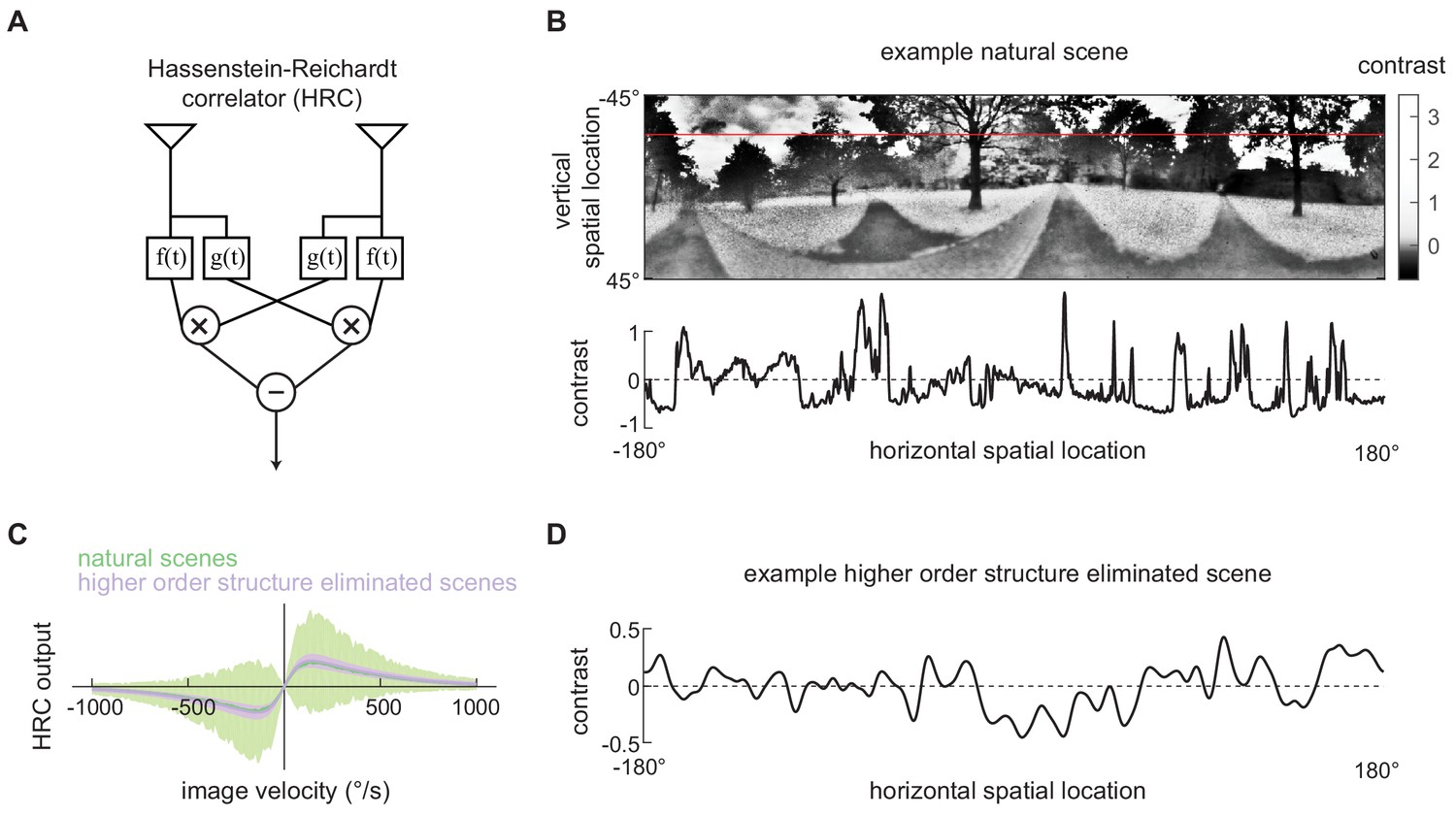
Second-order motion detectors perform poorly with natural scene inputs.
(A) Schematics of the Hassenstein-Reichardt correlator (HRC). Each half of the HRC receives inputs from two nearby points in space, which are filtered in time with filters and , and then multiplied together. The full HRC receives outputs from two symmetric halves with opposite direction tuning and subtracts two outputs. (B) An example two-dimensional photograph from a natural scene dataset (top), including a one-dimensional section (image) through the photograph (bottom), indicated by the red line. So that the image can be viewed clearly, the contrasts in the photograph were mapped onto gray levels so that an equal number of pixels were represented by each gray level. (C) Average response (line) and variance (shaded) of the outputs of an HRC (equivalent to a motion energy model; Adelson and Bergen, 1985) when presented with naturalistic motion at various velocities. Images were sampled from natural scenes (green) or from a synthetic image dataset in which all higher order structure was eliminated (purple, see Materials and methods). (D) Example synthetic image in which all higher order structure was eliminated.
Figure 1—figure supplement 1

Converting luminance signals into contrast signals (see Materials and methods).
(A) An example two-dimensional luminance photograph (upper) from the dataset, including a one-dimensional section through the photograph (bottom), indicated by the red line. The luminance is shown in log scale in the 1-dimensional image. (B) The two-dimensional photograph from (A) filtered with a two-dimensional Gaussian filter (FWHM = 5.3°) to represent the spatial filtering of the fly’s ommatidia. This yielded the photograph . (C) The two-dimensional photograph from (B) filtered with a two-dimensional Gaussian filter (FWHM = 25°) to represent local mean luminance. The white circle represents the FWHM of the filter. This yielded the photograph . (D) The two-dimensional photograph from (A) in units of contrast. We calculated the contrast by computing .
Figure 2 with 1 supplement
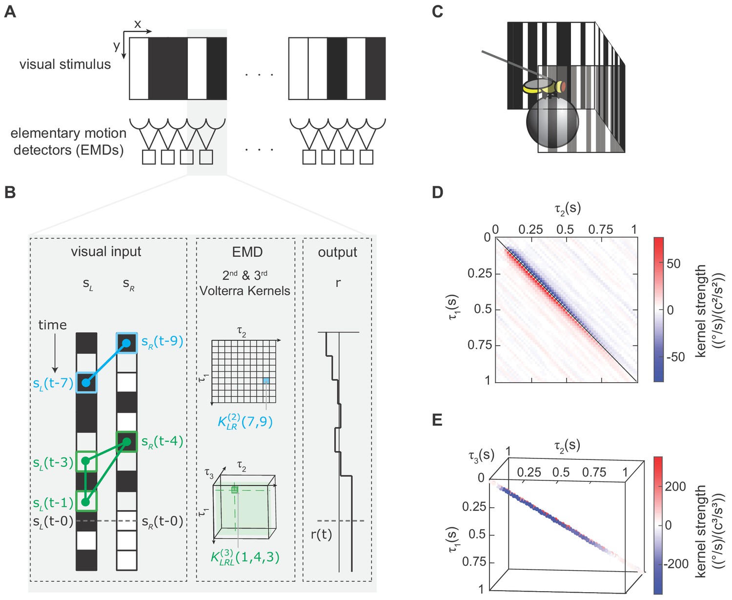
We modeled the fly’s motion computation algorithm with second- and third-order Volterra kernels and extracted the kernels using reverse-correlation (Appendix 1, Materials and methods).
(A) Visual depiction of our model, where the fly’s motion computation system consists of a spatial array of elementary motion detectors (EMDs), and each EMD receives inputs from two neighboring spatial locations. We presented flies with vertically uniform stimuli with 5°-wide pixels, roughly matching ommatidium spacing. (B) Diagram showing how the output of one EMD at time , indicated by gray dashed line, is influenced by the second- and third-order products in the stimulus. Left: visual inputs of one EMD, and . The visual stimulus contained products of pairwise and triplet points with various spatiotemporal structure. One specific pairwise product is highlighted (blue barbell) and one specific triplet product is highlighted (green triangle). Middle: The motion computation of the EMD is approximated by the second-order kernel (blue) and the third-order kernel (green). The second-order kernel (blue) is a two-dimensional matrix. For example, the response at time is influenced by the products of and with weighting . The third-order kernel (green) is a three-dimensional tensor. The response at time is influenced by with weighting . Right: turning response at time is influenced by all pairwise and triplet products in the visual stimulus, with weightings given by the second- and third-order kernel elements. (C) Diagram of the fly-on-a-ball rig. We tethered a fly above a freely-rotating ball, which acted as a two-dimensional treadmill. We presented stochastic binary stimuli, and measured fly turning responses. (D) The extracted second-order kernel. The color represents the magnitude of the kernel, with red indicating rightward turning and blue indicating leftward turning to positive pairwise spatiotemporal correlations. Above the diagonal line, the matrix represented left-tilted pairwise products (example in B) and below the diagonal line represents right tilted pairwise products. (E) The extracted third-order kernel. For visualization purposes, we show only the two diagonals with the largest magnitude.
Figure 2—figure supplement 1
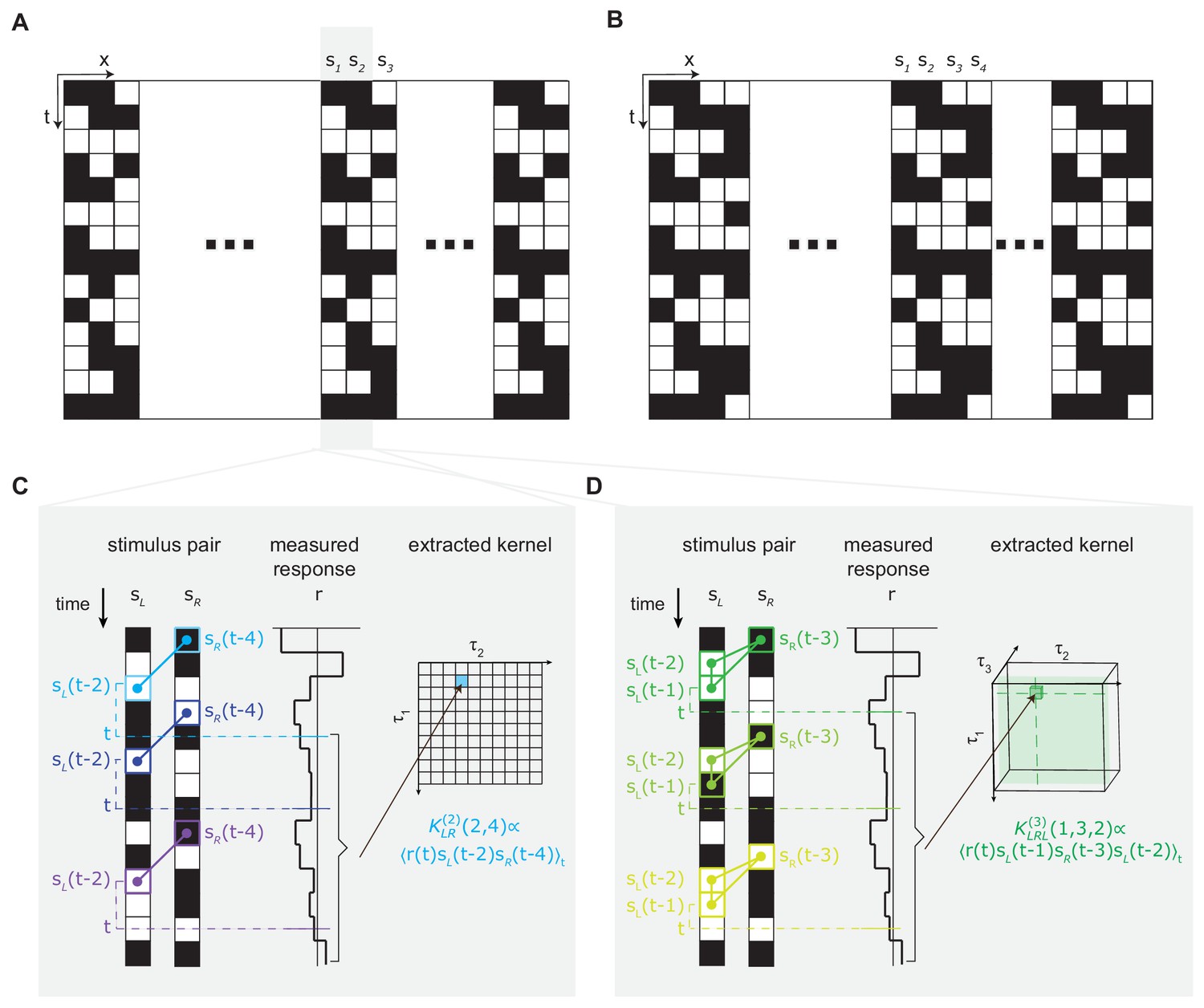
Using reverse-correlation to extract second- and third-order kernels from the measured turning response to stochastic binary stimulus (Materials and methods, Appendix 1).
(A) The three-bar-block stochastic binary stimulus (Materials and methods). The screen is 270° wide, and discretized into 5° bars. Within each three-bar-block, contrasts of three bars were randomly and independently sampled to be black or white over space and time. The block repeats itself across space 18 times. (B) The four-bar-block stochastic binary stimulus (Materials and methods), and block repeated itself across space 14.5 times. (C) Extracting the second-order kernel using reverse correlation. Left: visual stimulus at two neighboring spatial locations and , and examples of a second-order feature at three different times . Middle: Measured optomotor turning response of a fly. Right: To calculate a given element () in the second-order kernel, we calculated the product between the turning response at time and the corresponding second-order feature , and averaged the products over all times . (D) Extracting the third-order kernel with reverse correlation. Left: visual stimulus at two neighboring spatial locations, and , and examples of the third-order feature at three different times . Middle: Measured optomotor turning response of a fly. Right: To measure a given element () in the third-order kernel, we calculated the product between the turning response at time and the corresponding third-order feature , and averaged the products over all times .
Figure 3 with 2 supplements
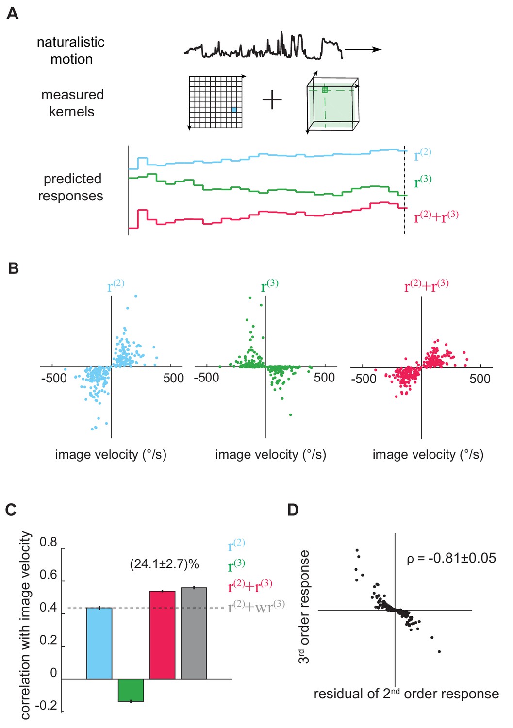
The third-order kernel improved motion estimation in natural scenes.
(A) Predicting responses of the second- and third-order kernels to rigidly moving scenes. Top: natural scenes rigidly translating with constant velocities. Middle: cartoon of the second- and third-order kernels. Bottom: second-order response (blue), third-order response (green), the predicted motion estimate (red) is the summation of and . (B) Scatter plot of and against image velocity over the ensemble of moving images. 10,000 independent trials were simulated, and 1000 trials were plotted here. (C) Pearson correlation coefficients between responses of each kernel and the true image velocities ( = 0.44 ± 0.01, -0.14 ± 0.01, 0.54 ± 0.01, 0.56 ± 0.01, from left to right; = 1.39 ± 0.01; mean ± SEM across 10 groups of 1000 trials). (D) Scatter plot between and the residual in , computed by subtracting a scaled image velocity from (Materials and methods). represents the Pearson correlation coefficient mean ± SEM across 10 groups (Materials and methods).
Figure 3—figure supplement 1
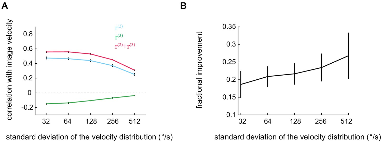
The improvement added by the third-order kernel persists across a wide range of velocities.
(A) Pearson correlation coefficient between the true image velocity and the second-order, third-order, and full outputs as a function of the standard deviation of the velocity distribution. (B) The improvement added by the third-order kernel as a function of the velocity standard deviation.
Figure 3—figure supplement 2
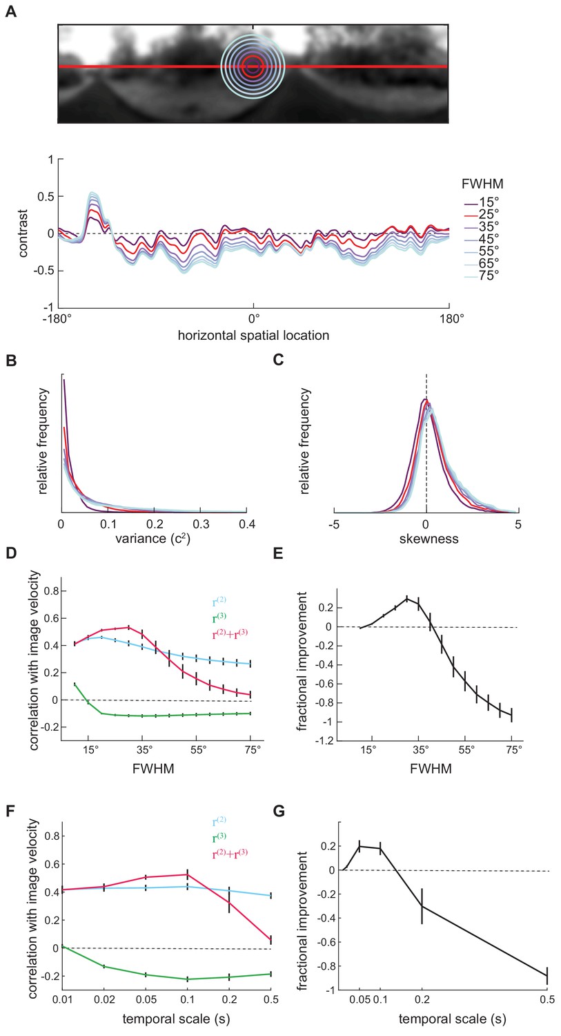
The length scale of local mean luminance computation affected the performance of the measured kernels.
(A) Local mean luminance was computed by filtering the luminance picture with a Gaussian filter (Materials and methods). We varied the full-width-half-maximum (FWHM) of this Gaussian filter from 15° to 75°. Top: Example two-dimensional blurred luminance photographs . The radius of the circle represents the length scale of the filter. Bottom: Example one-dimensional contrast images computed with corresponding filters. (B) As the length scale of the Gaussian filter increased, the distribution of the variances of individual images shifted to higher values. (C) As the length scale of the Gaussian filter increased, the distribution of the skewness of individual images shifted to more positive values. (D) The performance of measured kernels changed as the length scale of the Gaussian filter increased. (E) The improvement added by the third-order response to the second-order response existed when FWHM varied from 15° to 40°, and peaked around 30°. (F) The performance of second- and third-order responses as a function of the timescale of the contrast computation. (G) The degree of improvement added by the third-order responses changed with the timescale of the contrast computation.
Figure 4 with 3 supplements
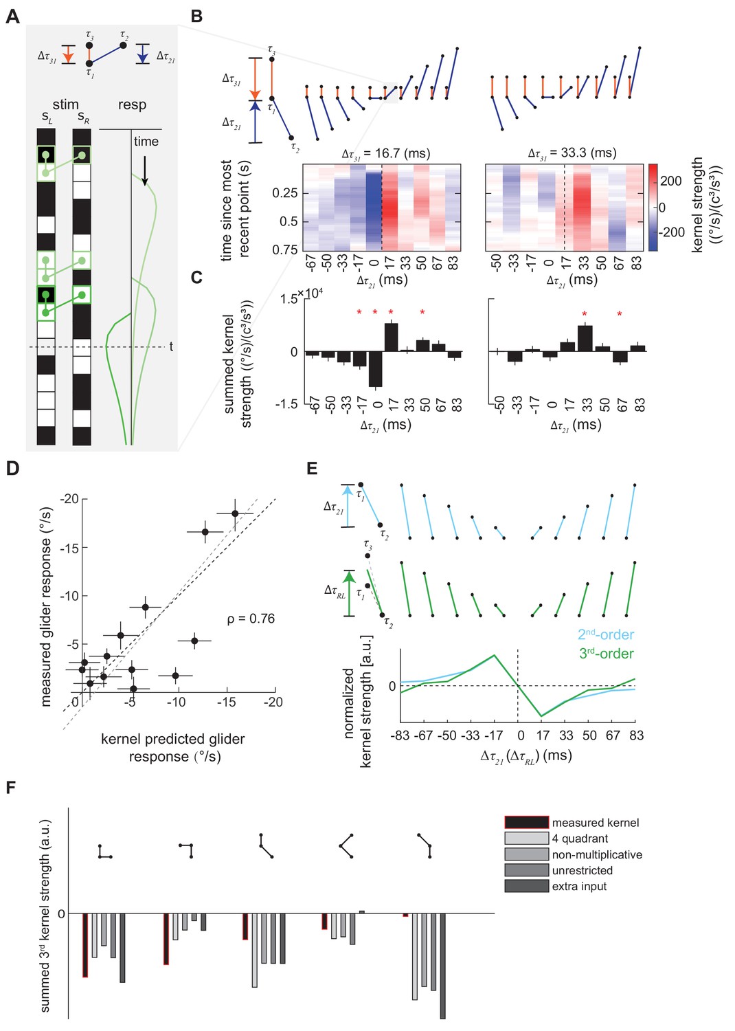
Characterization and validation of the measured third-order kernel.
(A) Triplet impulse response description. Top: the ball-stick diagram represents the relative spatiotemporal position of three points in a triplet. The red line denotes the temporal distance between the two left points, , and the blue line denotes the temporal distance between the more recent point on the left and the sole right point, . Bottom: Three specific example occurrences of the triplet elicit three impulse responses. The response at time is the sum of the impulse responses to all previous occurrences of the triplet. The first triplet (lightest green) involves two black points and one white point, so their product is positive, and it elicits an impulse response with positive sign. The triplet occurs far from current time , so its influence on the current response is small. The last triplet (darkest green) involves two white points and one black point, so the product is negative and it elicits an impulse response with flipped sign. It is close to current time , and has a large influence on the current response. (B) Third-order kernel visualized using an impulse-response format (Materials and methods). Top: the ball-stick diagrams as in (A). Bottom: the color map plots the 'impulse response' to the corresponding triplets, and color represents the strength of the kernel. Different panels represent different . In each color map, is fixed, the columns represent , and the rows represent the time since the most recent point in each triplet. The dashed lines indicate the place where the right point is in the middle of the two left points in time. (C) The summed strength of the third-order kernel along each column in A. Error bars represent SEM calculated across flies (n = 72), and significance was tested against the null kernel distribution (*p<0.05, two-tailed z-test (Materials and methods)). (D) The scatter plot between the measured responses to third-order glider stimuli (Materials and methods, Figure 4—figure supplement 1) against responses predicted by the third-order kernel (Materials and methods). The correlation between the predicted and measured responses is 0.76. Black dashed line is unity; gray dashed line is the best linear fit. (E) The measured second- and third-order kernel share temporal structures. Top: the ball-stick diagrams represent the relative spatiotemporal positions of the two points in each pair (blue), and three points in each triplet (green). Bottom: The kernel strength of the second-order kernel (blue) and third-order kernel (green) summed across all elements sharing the same spatiotemporal structures, that is summed over rows in Figure 4—figure supplement 2CD (Materials and methods). Figure 4—figure supplement 3, (F) The extracted third-order kernels from four optimized motion detectors (Fitzgerald and Clark, 2015) compared to the measured kernel from the fly. The summed kernel strength is summed across all elements which shared the same spatiotemporal structures diagramed above.
Figure 4—figure supplement 1
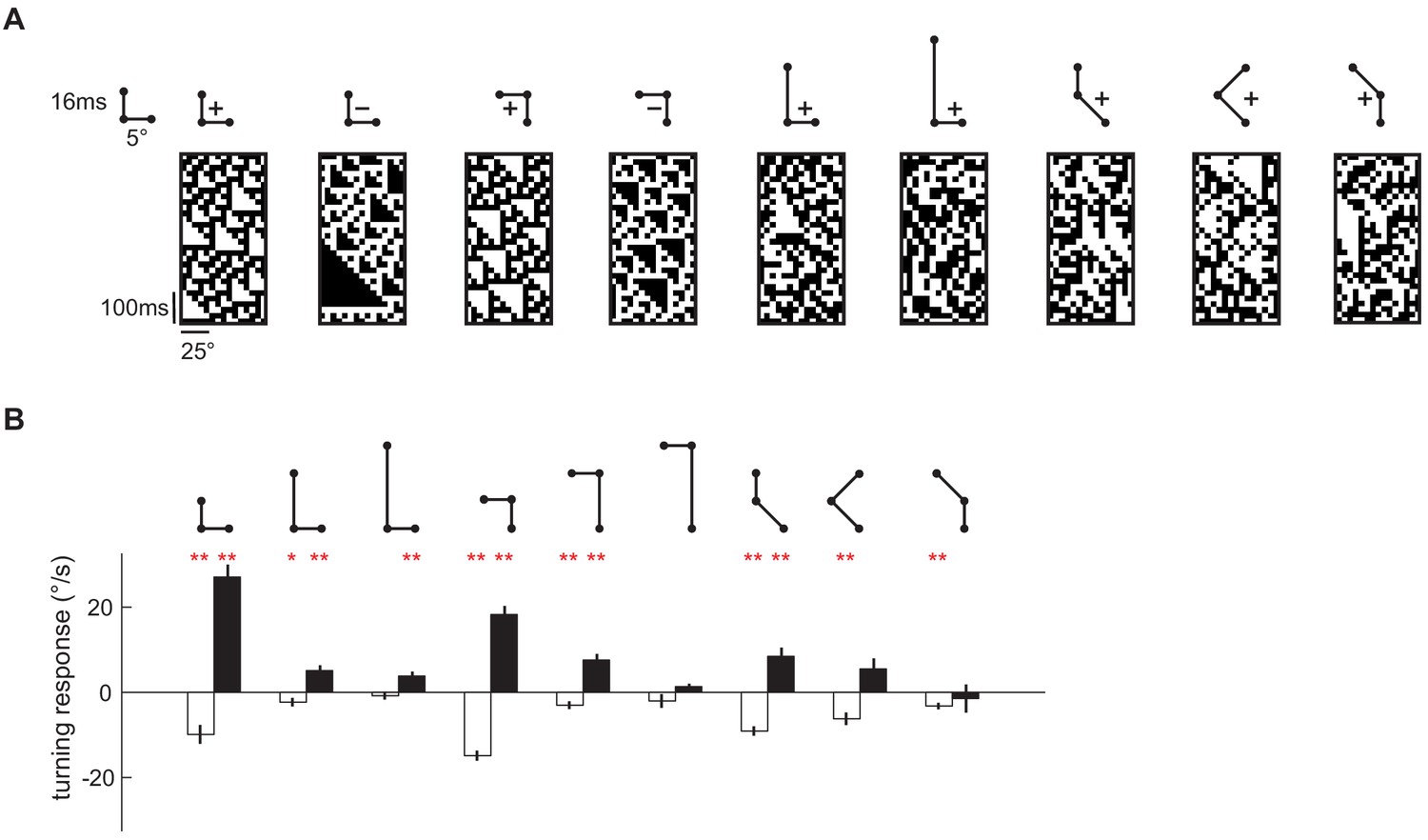
Flies turned in response to third-order spatiotemporal correlations presented in binary glider stimuli.
(A) Example space-time plots of third-order glider stimuli, in which the third-order spatiotemporal correlations were imposed. The ball-stick diagram above each space-time plot represents the relative spatiotemporal structure of the imposed triplet correlations. With the four-parameter scheme (Materials and methods), they are (from left to right): (1, 0, L, +1), (1, 0, L, −1), (1, 1, R, +1), (1, 1, R, −1), (2, 0, L, +1), (3, 0, L, +1), (1, −1, L,+1), (2, 1, R, +1), (1, 2, R, +1). (B) The white (black) bar represents the measured responses to the positive (negative) glider averaged across 'left' and 'right' gliders (Materials and methods). These correspond to gliders (from left to right): (1, 0, L, ±1) − (1, 0, R, ±1), (2, 0, L, ±1) − (2, 0, R, ±1), (3, 0, L, ±1) − (3, 0, R, ±1), (1, 1, R, ±1) − (1, 1, L, ±1), (2, 2, R, ±1) − (2, 2, L, ±1), (3, 3, R, ±1) − (3, 3, L, ±1), (1, −1, L, ±1) − (1, −1, R, ±1), (2, 1, R, ±1) − (2, 1, L, ±1), (1, 2, R, ±1) − (1, 2, L, ±1). The mean and SEM were calculated across flies. The p-values (**p<0.01, *p<0.05, Student t-test against null hypothesis of no response) and number of flies tested for each glider type is reported in Table 1.
Figure 4—figure supplement 2

Rearranging the second- and third-order kernels and computing singular value decompositions on the rearranged kernels.
(A) Diagrams to demonstrate how the third-order kernel was rearranged. The 'ball-stick' diagram represents the spatiotemporal structure of the triplet correlations. Left: is the average time difference between the left points and the right point, and is the temporal separation between two left points. In the grid, the rows represent in the unit of frame ms, and the columns represent . In the first row, the temporal distance between two left points is zero, so two left points overlap with each other, which is represented by a solid dot surrounded by an empty circle. The z-axis, which is not shown here, represents times since the most recent point. Right: Similar to left panel, but in this case, there are two points on the right and one point on the left. In the grid, the rows represent , and the columns represent . Positive means the left point is more recent than the right points (Materials and methods). (B) Two-dimensional representation of the third-order kernel by summing the rearranged third-order kernel elements in (A) and (B) over and (Materials and methods). In this new format, rows represent time since the most recent point, and columns describe the temporal distance between right and left points, with negative intervals meaning that the right point is more recent than the left point. (C) Two-dimensional representation of the third-order kernel created by summing neighboring columns in (B). (D) Second-order kernel visualized using an impulse-response format (Materials and methods). Top: the ball-stick diagrams represent the relative spatiotemporal structure of the pairwise spatiotemporal correlations. Bottom: the color map denotes the 'impulse response' to the corresponding pairs, and the color represents the kernel strength, the columns represent , and the rows represent the time since the most recent point in the pair. (E) Diagram of the singular value decomposition of a matrix. The matrix can be approximated by a series of outer products of vectors. (F) The singular values of the second-order kernel (blue) and the third-order kernel (green). (G) The optomotor turning response of the fly can be modeled as a correlation-sensitive module that represents motion computation and a low-pass filter module that represents the dynamical change of the turning behavior (Clark et al., 2011). The left vector (top) could be interpreted as the dynamics in a behavioral module and the right vector (bottom) as a correlation-sensitivity module.
Figure 4—figure supplement 3
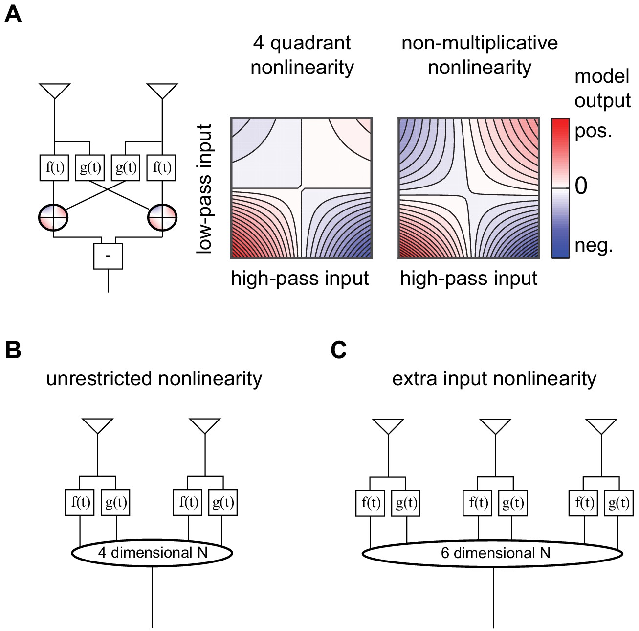
Four models optimized to estimate image velocities in natural scenes, adapted from Fitzgerald and Clark (2015).
(A) Four-quadrant and non-multiplicative model, these two models differ in the nonlinear interaction of the high- and low-pass inputs. (B) Unrestricted nonlinearity model, in which all interactions up to fourth-order were permitted between the four inputs from two points in space. (C) Extra input model, in which all interactions up to fourth-order were permitted between the six inputs from three points in space.
Figure 5 with 3 supplements
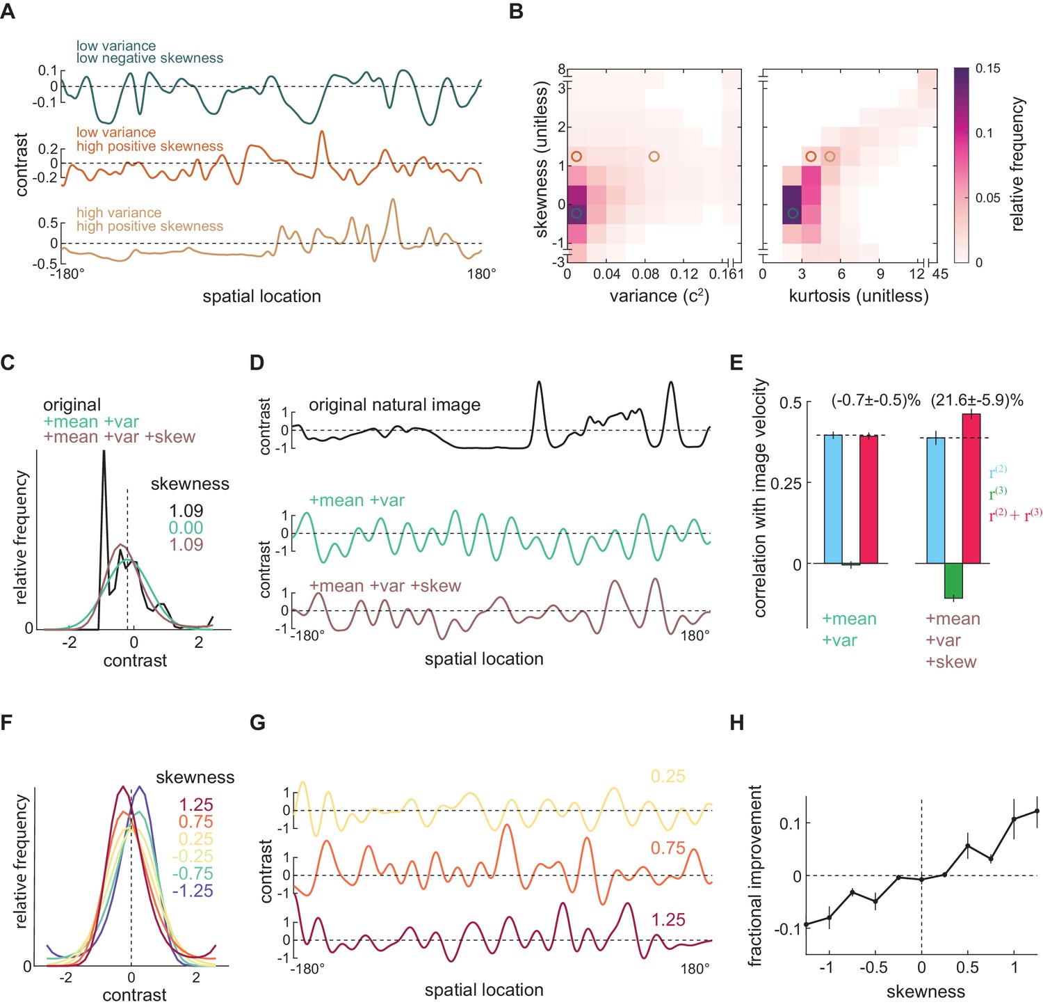
Positive skewness is sufficient for the third-order kernel to improve motion estimation.
(A) Three example natural scenes with different degrees of variance and skewness. (B) Joint-density maps of individual image statistics over the ensemble of natural images, showing the relationship between skewness and variance (left) and skewness and kurtosis (right). (C) Contrast distributions of example images from the natural scene dataset and two synthetic image datasets. The natural image is shown (black), along with a maximum entropy distribution (MED) with matched mean and variance, denoted by +mean +var (green) and an MED with matched mean, variance, and skewness, denoted by +mean +var +skew (brown). (D) Example images from the natural scene dataset and two synthetic image datasets corresponding to three contrast distributions in (C). (E) The Pearson correlation coefficient between true image velocities and each kernel’s responses in the two synthetic datasets +mean +var (green) and +mean +var +skew (brown) (F) Example of MEDs in six synthetic datasets, in which the image skewness ranged from −1.25 to 1.25. (G) Example of synthetic images in three synthetic datasets, corresponding to MEDs in (F) with constrained skewness of 0.25 (top), 0.75 (middle), and 1.25 (bottom). (H) Improvement added by the third-order response as a function of synthetic image skewness.
Figure 5—figure supplement 1
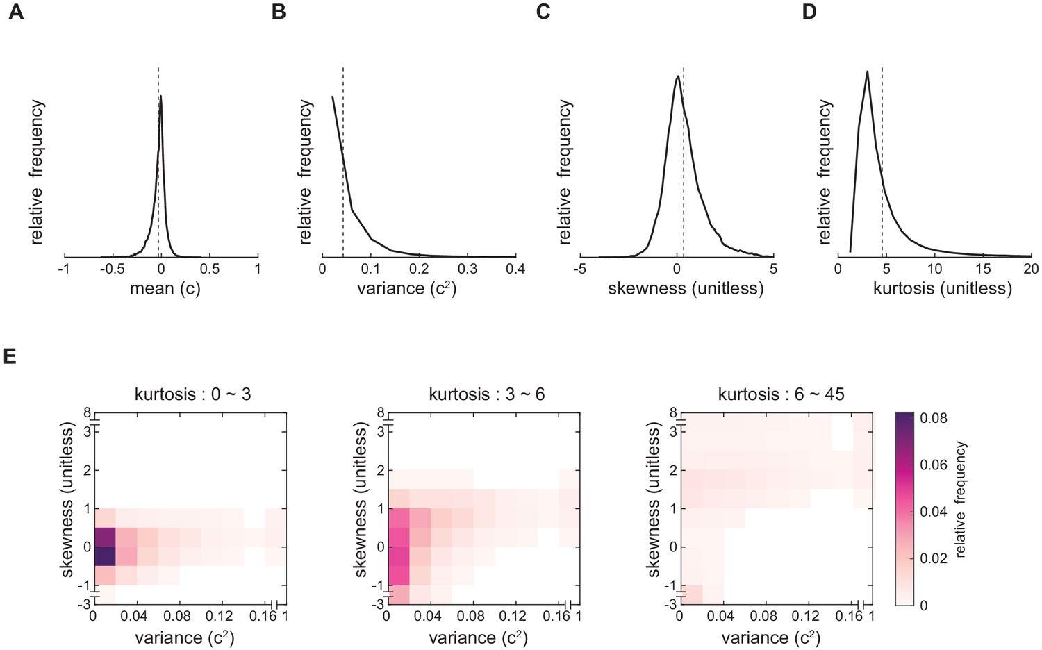
Natural scenes have heterogenous contrast statistics.
(A-D) Distribution of the contrast mean, variance, skewness and kurtosis of individual images within the entire natural scene ensemble. Mean is denoted by the vertical dashed line. (B) Image statistics are correlated with each other. Joint-density maps of variance and skewness with different ranges of kurtosis.
Figure 5—figure supplement 2
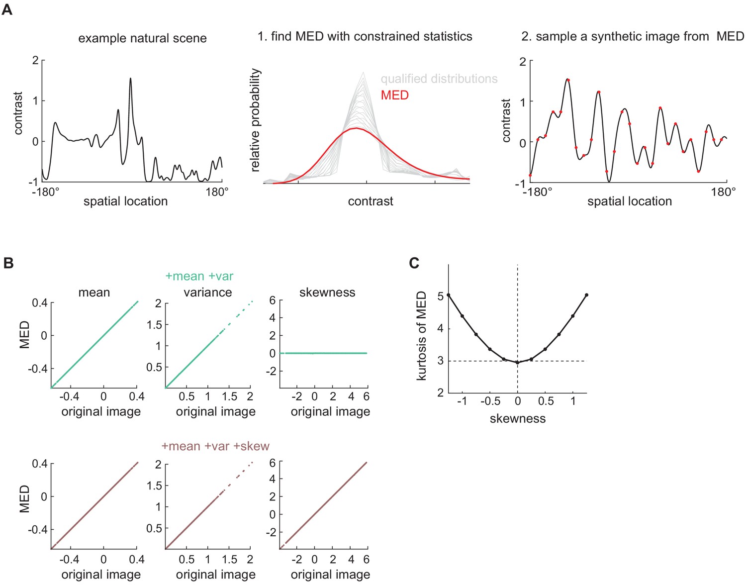
Using maximum entropy distributions (MEDs) to generate synthetic images with controlled image statistics.
(A) Two steps to generate one synthetic image with desired contrast statistics (Materials and methods, Appendix 2). Left: Select a natural image and calculate the mean, variance, and skewness of its contrast. Middle: There is a family of contrast distributions (gray) that have the same mean, variance, and skewness as the original natural image. One may use an optimization algorithm to find the distribution with the maximum entropy (red). Right: Sample-independent contrast values from the solved MED and interpolate between them to induce local spatial correlations. (B) Validating that the MEDs possessed the constrained statistics. Top row: When mean and variance were constrained, the mean and variance of the MEDs matched those of the original images. The skewness of the MEDs was zero. Bottom row: When mean, variance, and skewness were constrained, the mean, variance, and skewness of the MEDs matched those of the original images. (C) The kurtosis of the MEDs (Figure 5F) with skewness constrained to be different values.
Figure 5—figure supplement 3

The performance of the measured kernels in various synthetic image datasets.
(A) Scatter plots between the model responses and true image velocities when we constrained the synthetic images to match only the mean and variance of the natural images. (B) As in (A), but in this case, we also constrained the synthetic images to match the skewness of the natural image. (C) The performance of the measured kernels as skewness varied in synthetic datasets. (D) The correlation between the third-order responses and the residual in the second-order responses as a function of the skewness in synthetic datasets. (E) In comparison to Figure 5CD, where the contrast range of the MEDs matched the natural images, the contrast range of the MEDs here were fixed to be [−2.5, 2.5]. (F) Example images from these two distributions. (G) The Pearson correlation coefficients between the true image velocities and each kernel’s responses in the two synthetic datasets when the contrast range was fixed.
Appendix 2—figure 1
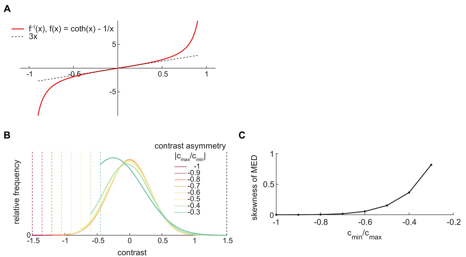
The shape of MED depends on the contrast range.
(A) The shape of function , where . (B) The mean-variance-constrained MED depends on the contrast range. The mean is constrained to be 0. The upper bound of the contrast range is fixed at 1.5, and the ratio of the lower-bound to upper bound changes from −1 to −0.2. As the contrast range becomes more asymmetric, the MED becomes more asymmetric. (C) When the contrast range is asymmetric, the mean-variance-constrained MED has induced non-zero skewness.
Tables
Table 1
Statistics of responses to third-order glider stimuli with different spatiotemporal structures.
| Index | (16 ms) | (16 ms) | () | () |
|---|---|---|---|---|
| 1 | 1 | 0 | (18, 12) | (0.0003, <0.0001) |
| 2 | 2 | 0 | (35, 29) | (0.0299, 0.0003) |
| 3 | 3 | 0 | (14, 8) | (0.4218, 0.0092) |
| 4 | 4 | 0 | (14, 8) | (0.0201, 0.3552) |
| 5 | 1 | 1 | (18, 13) | (<0.0001, <0.0001) |
| 6 | 2 | 2 | (35, 30) | (0.0026, <0.0001) |
| 7 | 3 | 3 | (14, 9) | (0.2323, 0.0875) |
| 8 | 4 | 4 | (14, 9) | (0.6778, 0.1700) |
| 9 | 1 | -1 | (8, 8) | (<0.0001, 0.0044) |
| 10 | 2 | 1 | (8, 8) | (0.0041, 0.0617) |
| 11 | 1 | 2 | (8, 8) | (0.0044, 0.6713) |
| 12 | 3 | 1 | (21, 21) | (0.5396, 0.4470) |
| 13 | 3 | 2 | (21, 21) | (0.1042, 0.0203) |
Table 2
Parameters for synthetic image datasets.
| Index of dataset | Imposed mean | Imposed variance | Imposed skewness | Contrast range | Discrete levels |
|---|---|---|---|---|---|
| MED-1 | NA | 32 | |||
| MED-2 | 32 | ||||
| MED-3 | 0 | 1.25 | 32 | ||
| MED-4 | 0 | 1 | 32 | ||
| MED-5 | 0 | 0.75 | 32 | ||
| MED-6 | 0 | 0.5 | 32 | ||
| MED-7 | 0 | 0.25 | 32 | ||
| MED-8 | 0 | −0.25 | 32 | ||
| MED-9 | 0 | −0.5 | 32 | ||
| MED-10 | 0 | −0.75 | 32 | ||
| MED-11 | 0 | -1 | 32 | ||
| MED-12 | 0 | −1.25 | 32 | ||
| MED-13 | 0 | NA | [-2.5, 2.5] | 512 | |
| MED-14 | 0 | [-2.5, 2.5] | 512 |
Table 3
Natural scene datasets for naturalistic motion simulations.
| Image dataset () | Velocity distribution (, or discrete values, °/s) | Number of trials | Motion Detector | |
|---|---|---|---|---|
| Figure 1C green | Natural scene (25°) | Discrete [0:10:1000] | 1000 each velocity | HRC |
| Figure 1C purple | Synthetic-higher order structure eliminated | Discrete [0:10:1000] | 1000 each velocity | HRC |
| Figure 3 | Natural scene (25°) | Gaussian (114) | 10000 | Fly |
| Figure 3—figure supplement 1 | Natural scene (25°) | Gaussian (32, 64, 128, 256, 512) | 8000 each velocity distribution | Fly |
| Figure 3—figure supplement 2DE | Natural scene (10° ~ 75°) | Gaussian (114) | 8000 each | Fly |
| Figure 3—figure supplement 2FG | Natural scene (10 ~ 500 ms) | Gaussian (114) | 8000 each | Fly |
| Figure 5CDE green, Figure 5—figure supplement 3A | Synthetic-MED-1 | Gaussian (114) | 8000 | Fly |
| Figure 5CDE brown Figure 5—figure supplement 3B | Synthetic-MED-2 | Gaussian (114) | 8000 | Fly |
| Figure 5FGH Figure 5—figure supplement 3CD | Synthetic-MED 5–14 | Gaussian (114) | 8000 each dataset | Fly |
| Figure 5—figure supplement 3G blue | Synthetic-MED-13 | Gaussian (114) | 8000 | Fly |
| Figure 5—figure supplement 3G red | Synthetic-MED-14 | Gaussian (114) | 8000 | Fly |
Additional files
Download links
A two-part list of links to download the article, or parts of the article, in various formats.
Downloads (link to download the article as PDF)
Open citations (links to open the citations from this article in various online reference manager services)
Cite this article (links to download the citations from this article in formats compatible with various reference manager tools)
Asymmetric ON-OFF processing of visual motion cancels variability induced by the structure of natural scenes
eLife 8:e47579.
https://doi.org/10.7554/eLife.47579


