The frequency limit of outer hair cell motility measured in vivo
- Erasmus MC, Netherlands
Figures
Figure 1 with 2 supplements
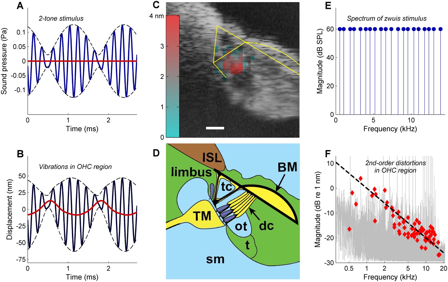
Rectification in the mechanical response of OHCs.
(A) Two-tone stimulus with primary frequencies 4600, 5400 Hz; 70 dB SPL. Blue line, waveform; dashed black lines, envelope; red line, lowpass-filtered waveform (2000-Hz cut-off). (B) Mechanical displacement evoked by the two-tone stimulus, recorded in the gerbil OHC/Deiters’ cell region (13 kHz CF). Black line, displacement waveform; dashed black lines, envelope. Rectification is illustrated by the red line obtained by low-pass filtering (2000-Hz cut-off). Positive polarity indicates displacement away from the measurement probe, that is vertically downwards in (C) and (D). (C) OCT reflectance image (grayscale), with structural framework of Corti’s organ (yellow) superimposed for reference. Color-coded overlay: total RMS value of 2nd-order distortion products (DP2s) evoked by a 12-tone complex, 2–12 kHz; 60 dB SPL. DP2s dominate in the OHC region. Scale bar, 0.025 mm. (D) Underlying anatomical structures. BM = basilar membrane; ISL = inner spiral lamina; sm = scala media; dc = Deiters’ cells; t = tectal cells; TM = tectorial membrane; tc = tunnel of Corti; ot = outer tunnel. Hair cells, dark blue. (E) Zwuis stimulus (see text). (F) Vibration spectrum recorded in OHC region in response to the zwuis stimulus. Red diamonds, Rayleigh-significant DP2s. Dashed line, 6-dB/octave roll-off.
-
Figure 1—source data 1
MATLAB binary file containing the data shown in Figure 1.
- https://doi.org/10.7554/eLife.47667.006
Figure 1—figure supplement 1
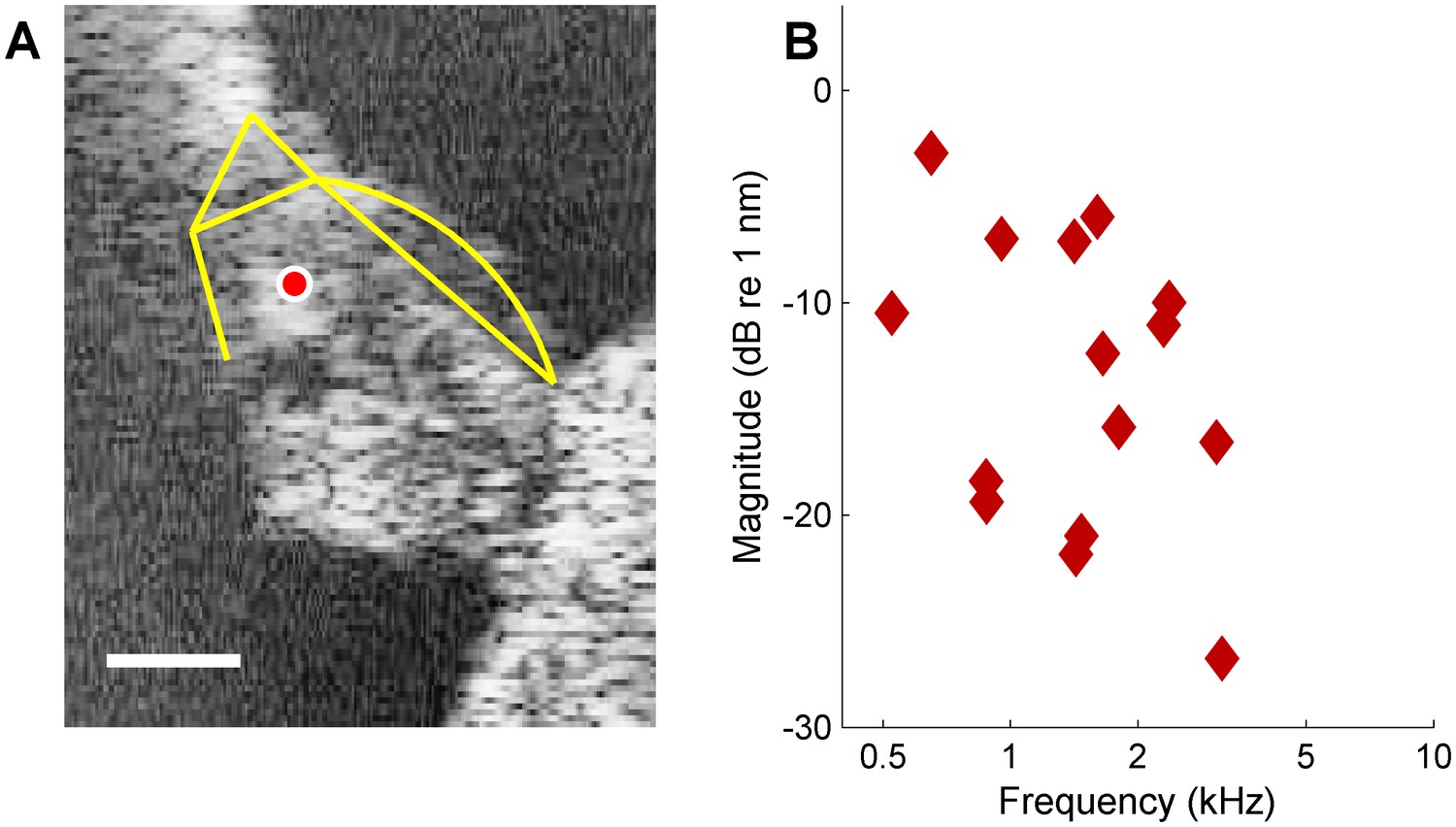
DP2s at low sound intensities.
(A) OCT reflectance image (grayscale), with structural framework of Corti’s organ (yellow) superimposed for reference. CF = 14 kHz. The red circle in the OHC/Deiters’ cell region marks the recording position. Scale bar, 0.05 mm. (B) Magnitude spectrum of Rayleigh-significant (p=0.001) DP2s evoked by a 43-component zwuis stimulus presented at 25 dB SPL per component, recorded at the position marked in panel (A).
Figure 1—figure supplement 2
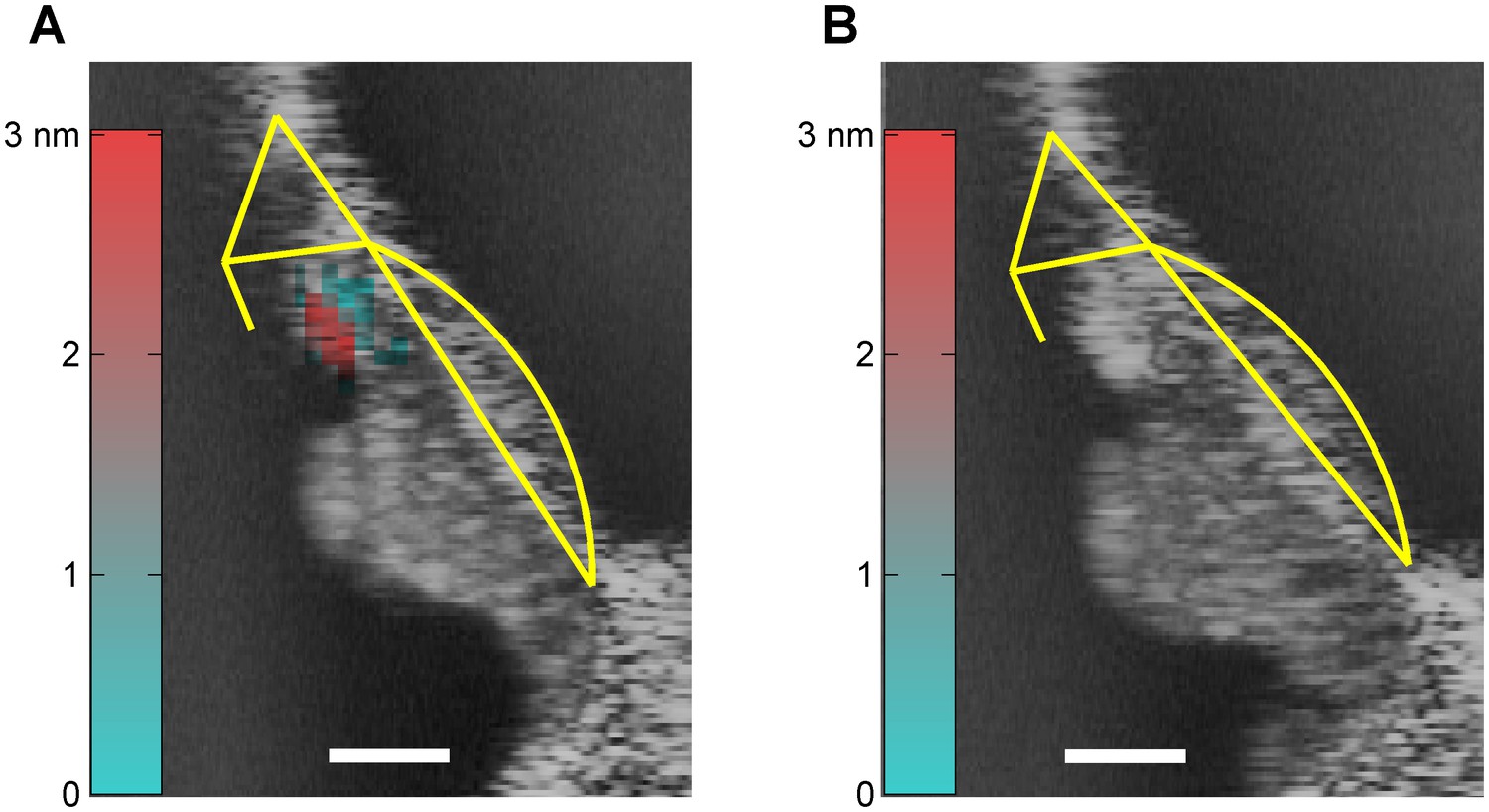
Post mortem disappearance of DP2s.
(A) In vivo OCT reflectance map (grayscale) of the organ of Corti (CF = 22 kHz) with with structural framework of Corti’s organ (yellow) superimposed for reference. Color-coded overlay: total RMS value of 2nd-order distortion products (DP2s) evoked by a 16-tone complex, 2-15 kHz; 65 dB SPL. DP2s dominate in the OHC region. Scale bar, 0.05 mm. (B) Same as (A) (identical stimulus, same ear), but recorded within 20 minutes post mortem. The DP2s have disappeared.
Figure 2 with 2 supplements
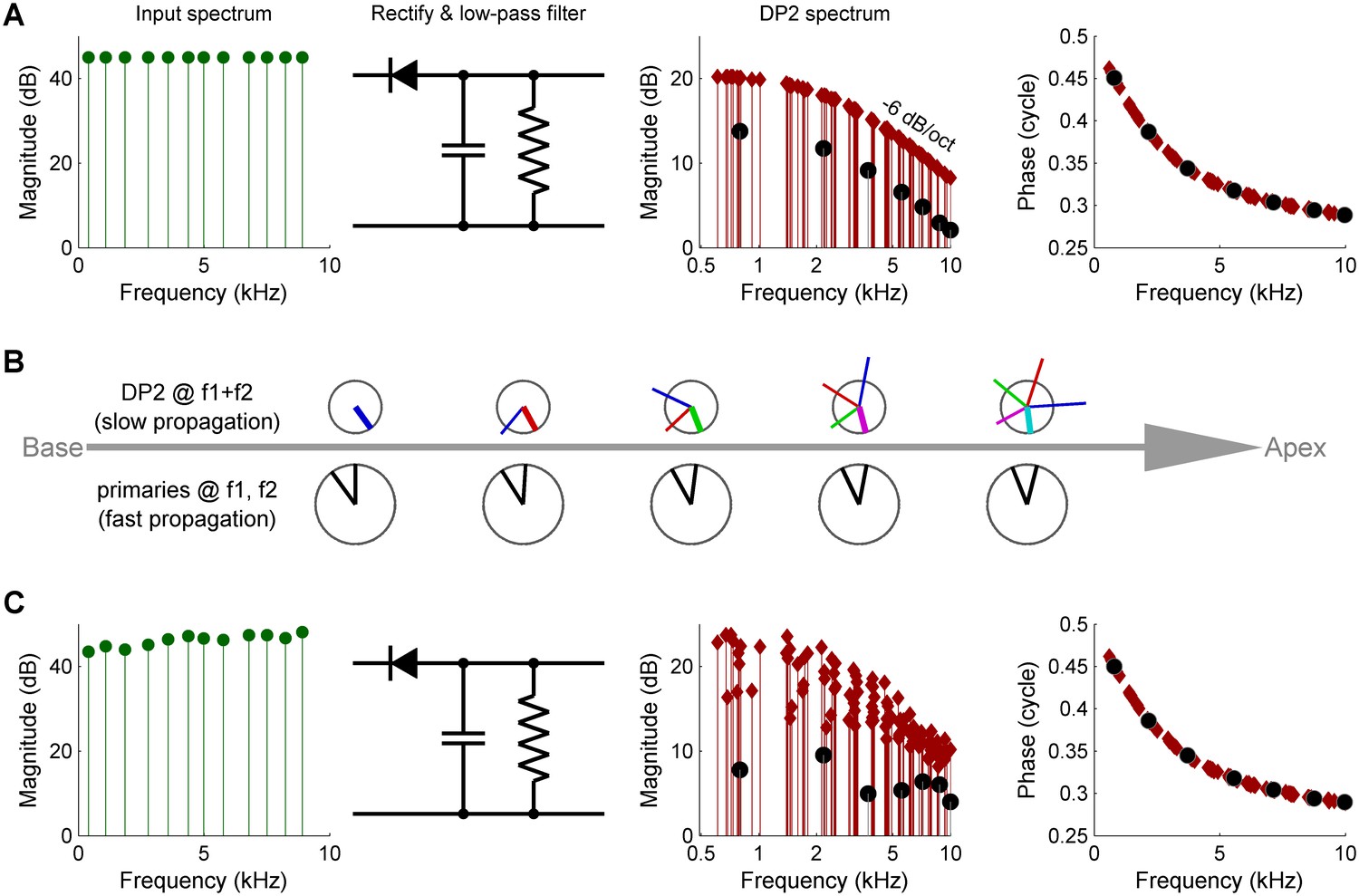
Three causes of magnitude scatter in DP2 spectra.
(A) Combinatorial effect illustrated by feeding an equal-amplitude zwuis tone complex to a nonlinear circuit comprising a rectifier and low-pass filter (corner frequency 2.5 kHz). The 2nd harmonics (solid circles) are 6 dB weaker than the remaining DP2s (red diamonds). (B) Vector addition of DP contributions along the traveling wave (left to right). Lower row of ‘clocks’ depict amplitude and phase of the primaries f1,f2 <<CF. They accumulate little phase and their amplitude hardly grows upon traveling. Upper clocks depict a near-CF DP2 at f1+f2. Colors indicate the origin of each local contribution. Near-CF DP2 components suffer considerable phase accumulation and amplitude variation while traveling. The eventual amplitude (rightmost location) is the vector sum of multiple contributions widely differing in phase and amplitude. This interference obfuscates the spectral properties of DP2 generation investigated here. (C) Unequal primary amplitudes entering the nonlinear circuit generate a predictable scatter in DP2 magnitudes (see text). Companion phases are not affected by lack of equalization of the input. The 0.5-cycle low-frequency limit of the phase reflects the ‘negative polarity’ of the rectification.
Figure 2—figure supplement 1
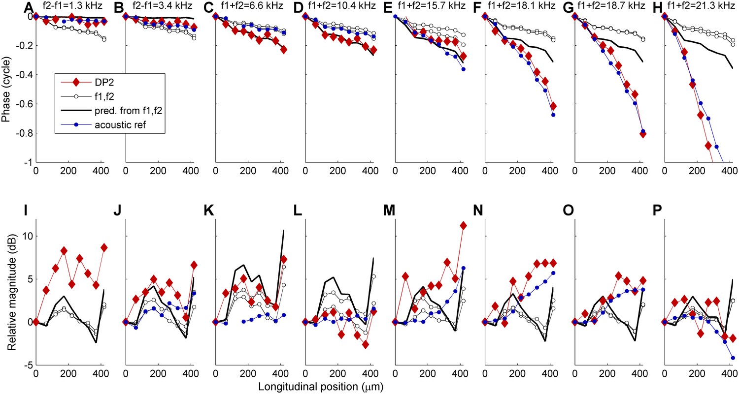
Propagation of DP2s in the 18-25-kHz region.
Recordings were made at 9 adjacent longitudinal locations spanning ~400 μm. Phase (upper row) and magnitude (lower row) are shown of: 6 example DP2 components (red diamonds); its two parent primaries f1 and f2 (open black circles); phase and amplitude predicted by Equation 1, that is assuming local generation (black line); a reference acoustically presented component of approximately the same frequency (blue circles). DP frequency is indicated above each phase graph. For the lowest DP2 frequencies (1.3-10.4 kHz) the actual DP2 phase matches the prediction within ~0.05 cycle. For the higher DP2 frequencies systematic deviations occur. The phase accumulation of the high-frequency DP2s matches the phase of the acoustic reference much better than the prediction based on local generation. Thus these high-frequency DP2 components are dominated by their own propagation rather than local contributions from the primaries as in Equation 1. The increasing dominance of propagation with increasing DP2 frequency was observed for all DP2s.
Figure 2—figure supplement 2
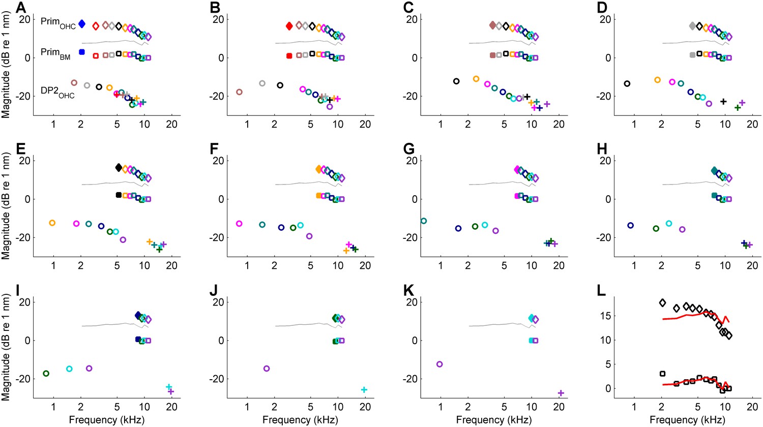
Comparison of linear response components and second-order distortion products (DP2s).
Data from recording shown in the lowest curves in Figure 4A–C (CF = 25 kHz; estimated cutoff frequency, 3006 Hz). (A–K) The DP2s are split according to their ‘heritage’ and the linear response components (‘parents’) are also shown. In A all the DP components relating to the lowest primary are shown. In B, that lowest primary is excluded and all the DP components relating to the new lowest primary are shown, and so on through panel K. Diamonds, linear response component (primary response) measured in the hotspot (OHC/Deiters’ region). Squares, primary response measured on the basilar membrane (BM). Circles, difference tones at f2- f1 measured in the hotspot. Plus signs, sum tones at f1+ f2 measured in the hotspot. The solid lines in all panels are identical; they show the effective OHC input determined from the DP2 spectrum. Their overall magnitude is unknown; the vertical position of the curves is chosen halfway the linear responses of BM and hotspot to facilitate comparison. The DP2s are split according to the lower primary f1. The filled symbol in each panel marks the f1 of all the DP2 components in that panel. The colors of the DP2s at f1+ f2 (plus signs) and f2- f1 (circles) match the colors of the linear responses at f2 in the same panel. (L) Detailed comparison between effective OHC input and primary responses. The effective OHC input (red lines) is shown at two different vertical positions: shifted for maximum overlap with primary responses at the hotspot (diamonds) and the BM (squares). The overlap is better for the BM data (RMS deviation, 0.9 dB) than for the hotspot data (RMS deviation, 1.9 dB).
Figure 3
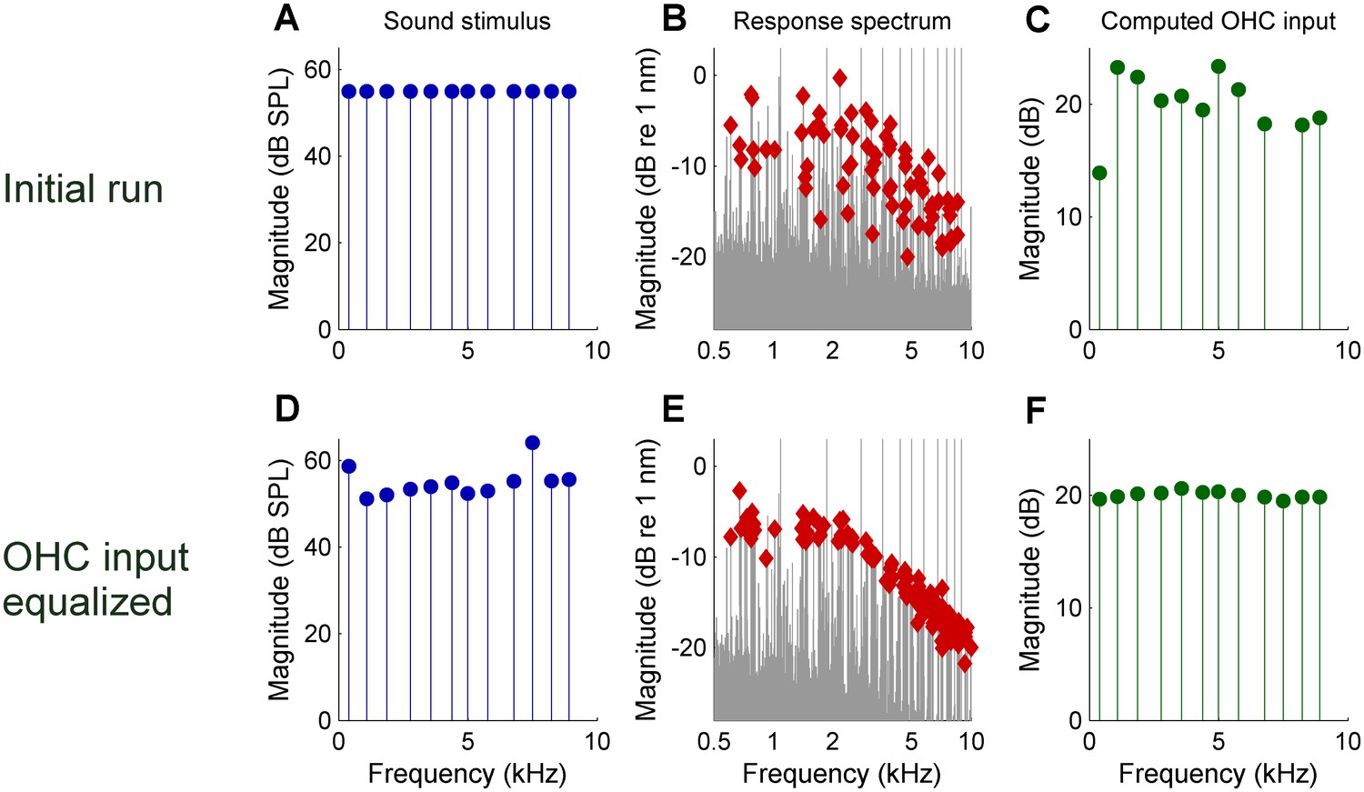
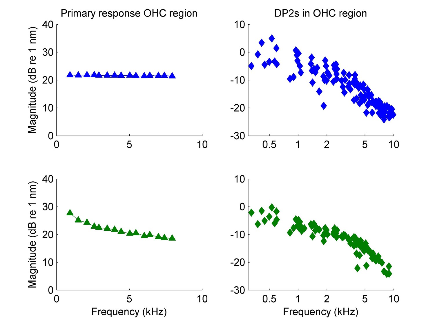
Reducing the scatter of DP2 magnitudes by equalizing the effective OHC input during an experiment.
(A) Spectrum of the initial zwuis acoustic stimulus. (B) Spectrum of the vibrations recorded in the OHC region; CF = 16 kHz. Rayleigh-significant DP2s marked as red diamonds; 2nd harmonics corrected for the 6-dB combinatorial effect. (C) Effective OHC input computed from the DP2 magnitudes. (D) Spectrum of the adapted stimulus (4th iteration) aimed at equalizing the effective OHC input. (E) Resulting DP2 spectrum. (F) Effective OHC input. Note that the equalized input spectrum in F (compared to C) reduces the DP2 scatter in E (compared to B).
-
Figure 3—source data 1
MATLAB binary file containing the data shown in Figure 3.
- https://doi.org/10.7554/eLife.47667.011
Figure 4 with 1 supplement

Low-pass filtering and corner frequencies of OHCs.
(A) DP2 magnitude versus frequency measured across different cochleas at different CFs. Stimuli, 10–12 component zwuis not exceeding CF/2; component intensities 55–65 dB SPL, optimized to equalize OHC input. Individual curves are offset to avoid overlap; labeled straight lines indicate absolute displacement. CFs, see legend of panel D. Second harmonics were corrected for the 6-dB combinatorial deficiency. (B) The same magnitudes corrected post-hoc for the effects of residual magnitude inequality in the effective input (see Appendix 1—figure 3). Black lines, first-order low-pass filters fitted jointly to the magnitude and phase data of each recording. (C) Companion phase data: the difference between the recorded DP2 phases and the predictions obtained by adding or subtracting the primary phases of the OHC input (Appendix 1, Equation 3B). Black lines, phase curves of the fitted low-pass filters. (D) Corner frequencies from the fits versus CF. Symbols as in panels A-C. Open circles reproduce in vitro data from Johnson et al. (2011). Dashed line, unity line (corner frequency = CF). Explained variance of the fits (in order of increasing CF): 90%, 91%, 80%, 85%, 87%. When omitting the correction for residual scatter, and instead using the raw magnitudes from panel A, the estimates of the corner frequencies were lower by 1% to 10% (mean, 7%) compared to the estimates based on the corrected magnitudes. Captions of source Data.
-
Figure 4—source data 1
MATLAB binary file containing the data shown in Figure 4.
- https://doi.org/10.7554/eLife.47667.014
Figure 4—figure supplement 1
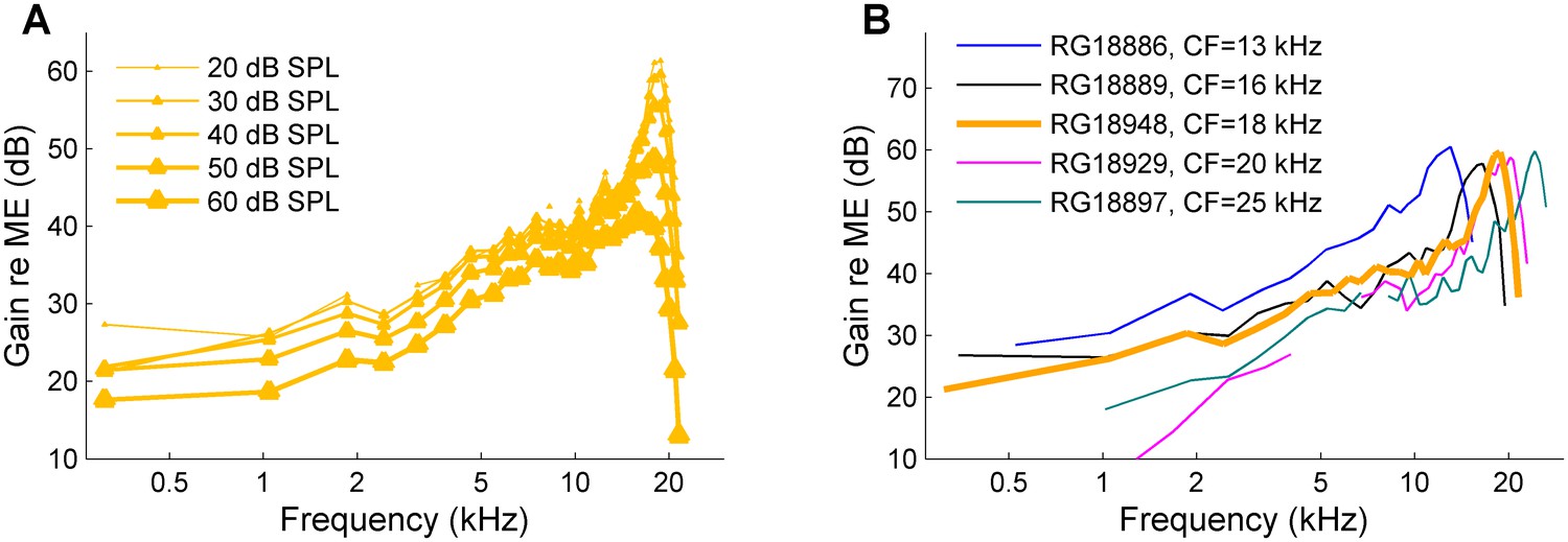
Sensitivity of the cochleae.
(A) a set of responses to a wideband zwuis stimuli at multiple SPLs as indicated in the graph, recorded from the CF = 18 kHz cochlea of Figure 4. The curves display the familiar compressive behavior of sensitive cochleae. (B) 30-dB-SPL recordings obtained from all five cochleae displayed in Figure 4, using the same colors as in that figure.
Appendix 1—figure 1
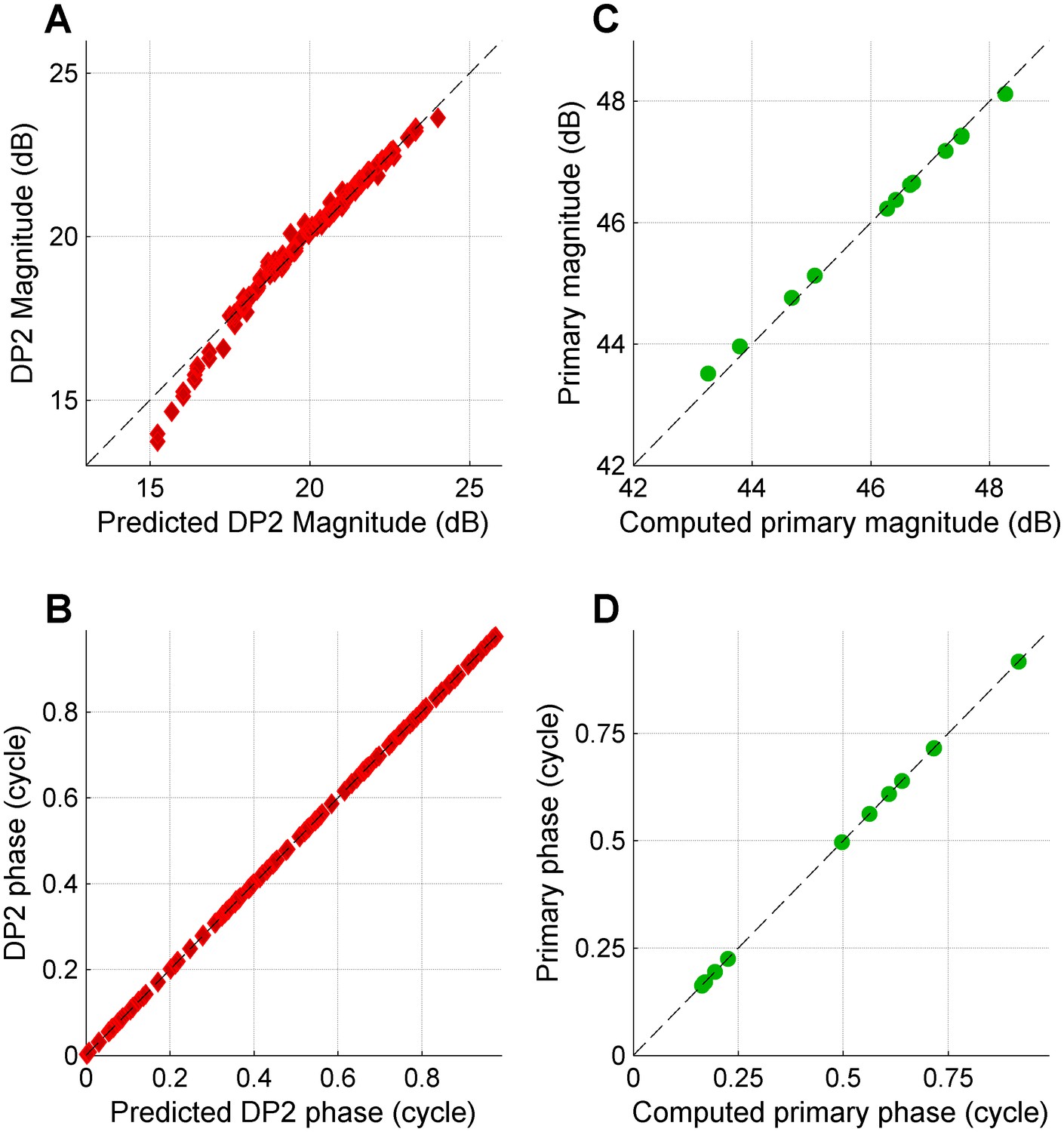
Predicting the DP2 spectrum from a primary spectrum and vice versa; no low-pass filtering.
(A) Actual DP2 magnitudes obtained by rectifying (not followed by filtering) the tone complex with unequal primary magnitudes shown in Figure 2C, left panel, plotted against the approximation of Equation 1. (B) As in (A), but now for the phase. (C) Retrieving the primary magnitudes from the DP2 spectrum by inverting (fitting) Equation 1. Actual primary magnitudes are plotted versus computed magnitude. (D) As in (C), but now for the phase.
Appendix 1—figure 2
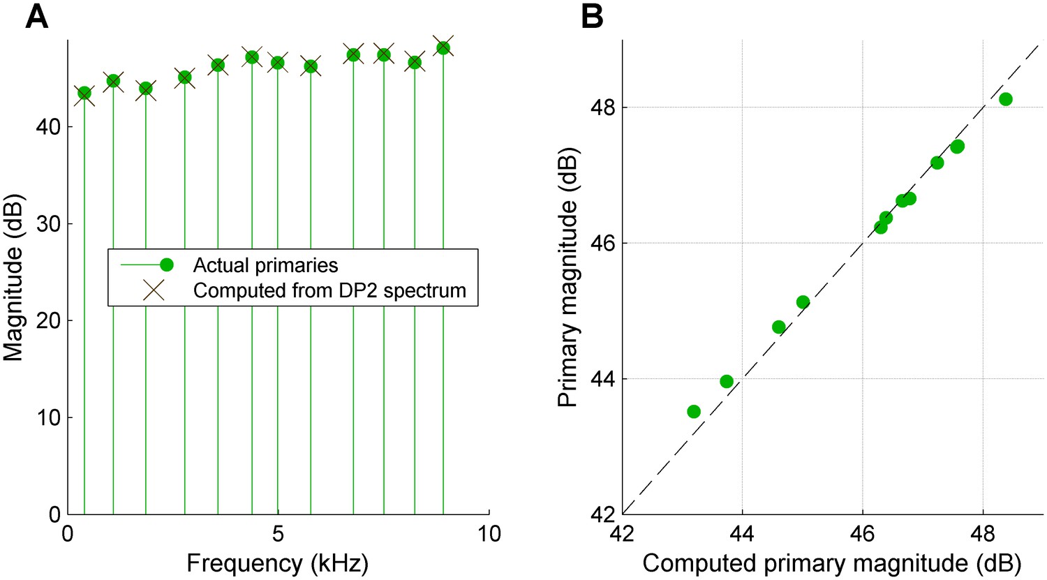
Retrieving the primary spectrum from the low-pass filtered DP2 spectrum.
(A) A tone complex with non-equalized primary spectrum (green circles) was rectified and low-pass filtered at 2.5 kHz. From the resulting DP2 spectrum, the primary spectrum was reconstructed (black Xs). (B) Scatter plot comparing the actual primary spectrum entering the rectifier + low-pass filter scheme to the primary spectrum reconstructed from the DP2 spectrum at the output of the low-pass filter.
Appendix 1—figure 3
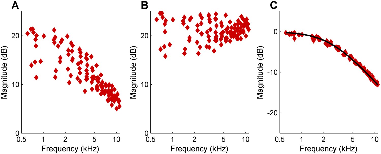
Computational separation of DP2 scatter and filter effect.
(A) DP2 spectrum obtained by rectifying and low-pass filtering a zwuis multitone waveform having unequal primary amplitudes. (B) Magnitude scatter in the DP2 spectrum of panel (A), computed by inserting the retrieved primary magnitudes into Equation 1. (C) The effect of the low-pass filter isolated by subtracting the scatter contribution of panel (B) from the DP2 spectrum in (A). For reference, the gain curve of actual filter that was used to generate the DP2 spectrum (first-order low-pass; corner frequency 2.5 kHz) is also shown (black line).
Author response image 1
Author response image 2

Additional files
-
Transparent reporting form
- https://doi.org/10.7554/eLife.47667.015
Download links
A two-part list of links to download the article, or parts of the article, in various formats.
Downloads (link to download the article as PDF)
Open citations (links to open the citations from this article in various online reference manager services)
Cite this article (links to download the citations from this article in formats compatible with various reference manager tools)
The frequency limit of outer hair cell motility measured in vivo
eLife 8:e47667.
https://doi.org/10.7554/eLife.47667


