DeepPoseKit, a software toolkit for fast and robust animal pose estimation using deep learning
- Max Planck Institute of Animal Behavior, Germany
- University of Konstanz, Germany
- Princeton University, United States
- Technische Universität München, Germany
Figures
Figure 1 with 1 supplement
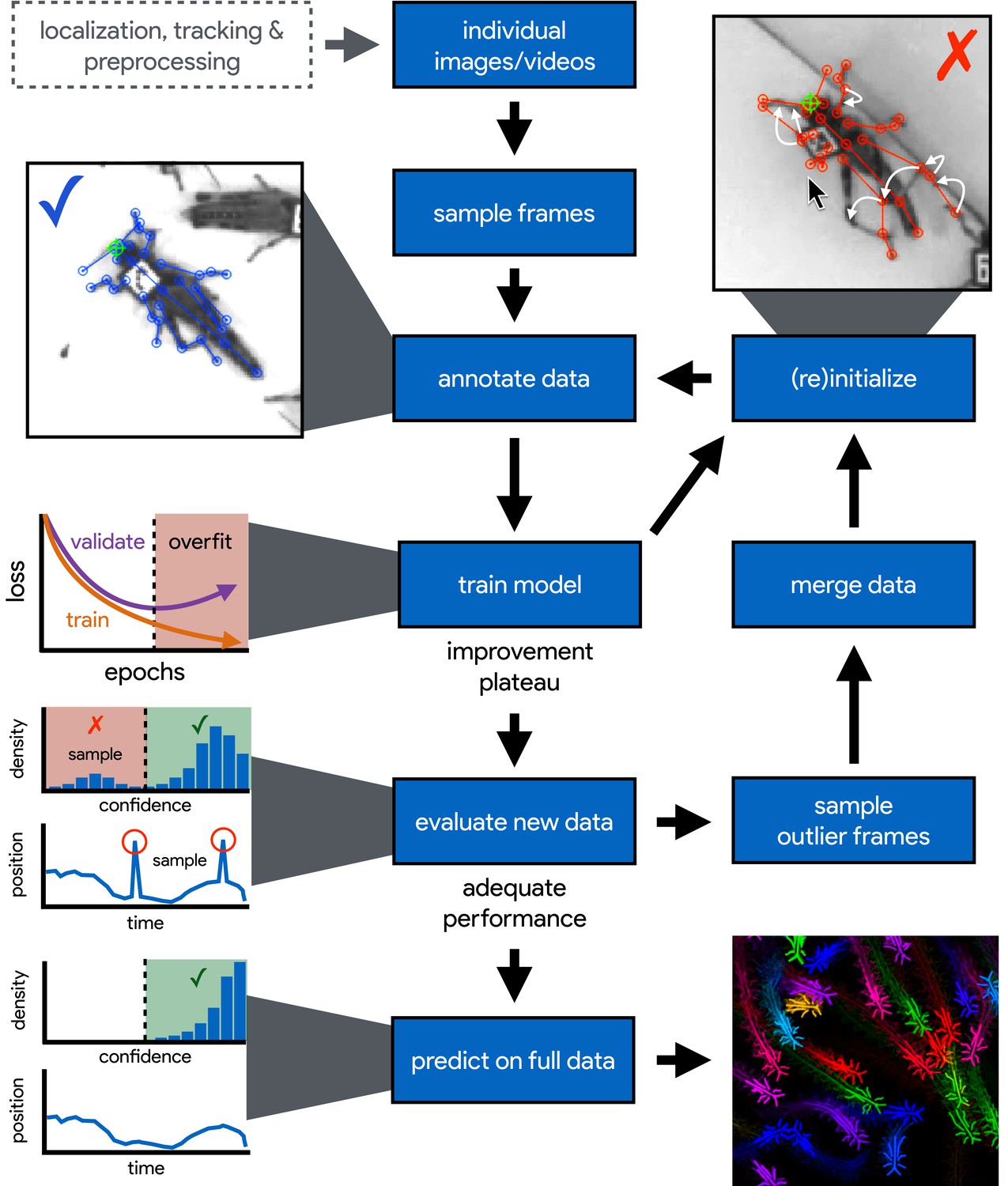
An illustration of the workflow for DeepPoseKit.
Multi-individual images are localized, tracked, and preprocessed into individual images, which is not required for single-individual image datasets. An initial image set is sampled, annotated, and then iteratively updated using the active learning approach described by Pereira et al. (2019) (see Appendix 3). As annotations are made, the model is trained (Figure 2) with the current training set and keypoint locations are initialized for unannotated data to reduce the difficulty of further annotations. This is repeated until there is a noticeable improvement plateau for the initialized data—where the annotator is providing only minor corrections—and for the validation error when training the model (Appendix 1—figure 4). New data from the full dataset are evaluated with the model, and the training set is merged with new examples that are sampled based on the model’s predictive performance, which can be assessed with techniques described by Mathis et al. (2018) and Nath et al. (2019) for identifying outlier frames and minimizing extreme prediction errors—shown here as the distribution of confidence scores predicted by the model and predicted body part positions with large temporal derivatives, indicating extreme errors. This process is repeated as necessary until performance is adequate when evaluating new data. The pose estimation model can then be used to make predictions for the full data set, and the data can be used for further analysis.
Figure 1—video 1
A visualization of the posture data output for a group of locusts (5× speed).
Figure 2
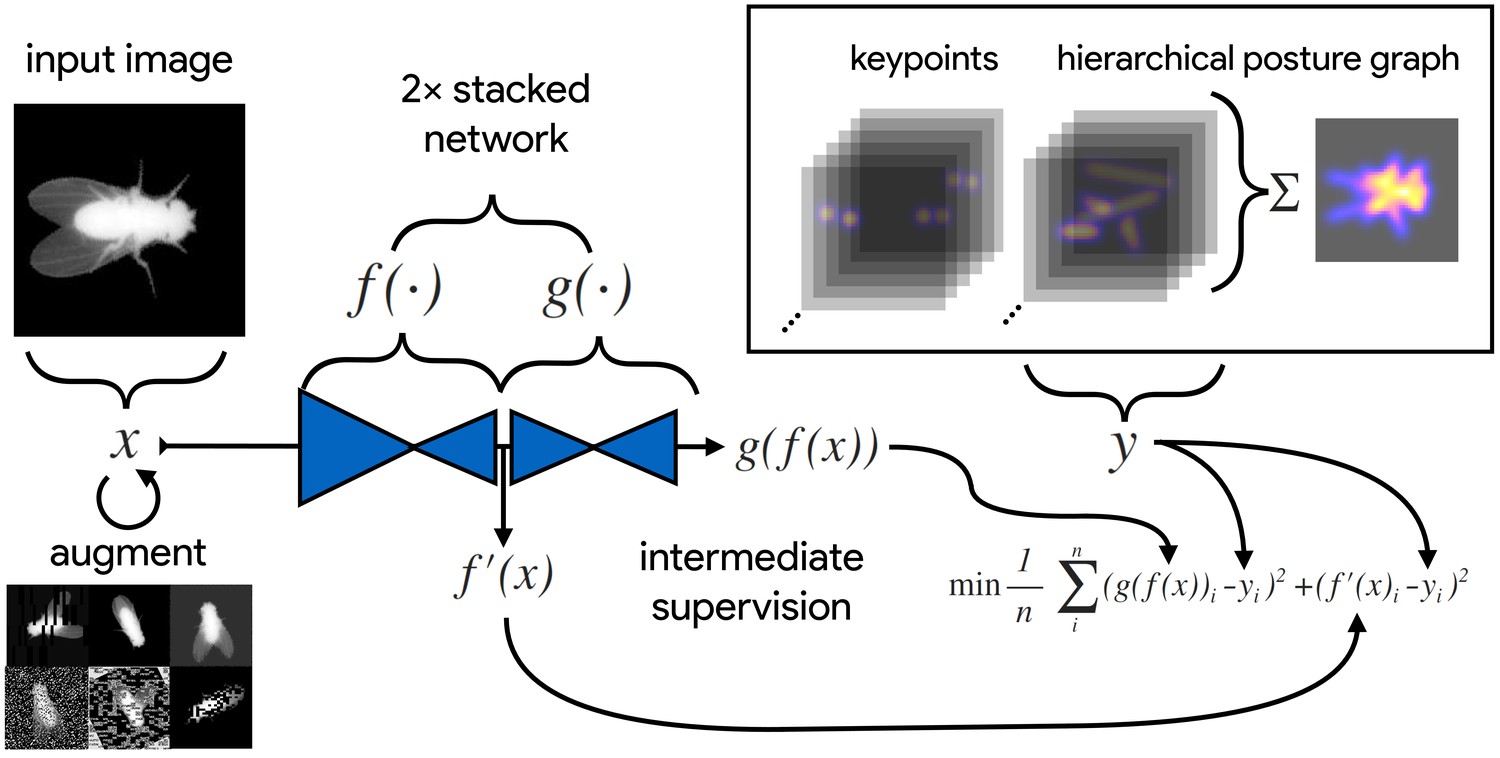
An illustration of the model training process for our Stacked DenseNet model in DeepPoseKit (see Appendix 2 for details about training models).
Input images (top-left) are augmented (bottom-left) with various spatial transformations (rotation, translation, scale, etc.) followed by noise transformations (dropout, additive noise, blurring, contrast, etc.) to improve the robustness and generalization of the model. The ground truth annotations are then transformed with matching spatial augmentations (not shown for the sake of clarity) and used to draw the confidence maps for the keypoints and hierarchical posture graph (top-right). The images are then passed through the network to produce a multidimensional array —a stack of images corresponding to the keypoint and posture graph confidence maps for the ground truth . Mean squared error between the outputs for both networks and and the ground truth data is then minimized (bottom-right), where indicates a subset of the output from —only those feature maps being optimized to reproduce the confidence maps for the purpose of intermediate supervision (Appendix 5). The loss function is minimized until the validation loss stops improving—indicating that the model has converged or is starting to overfit to the training data.
Figure 3 with 1 supplement
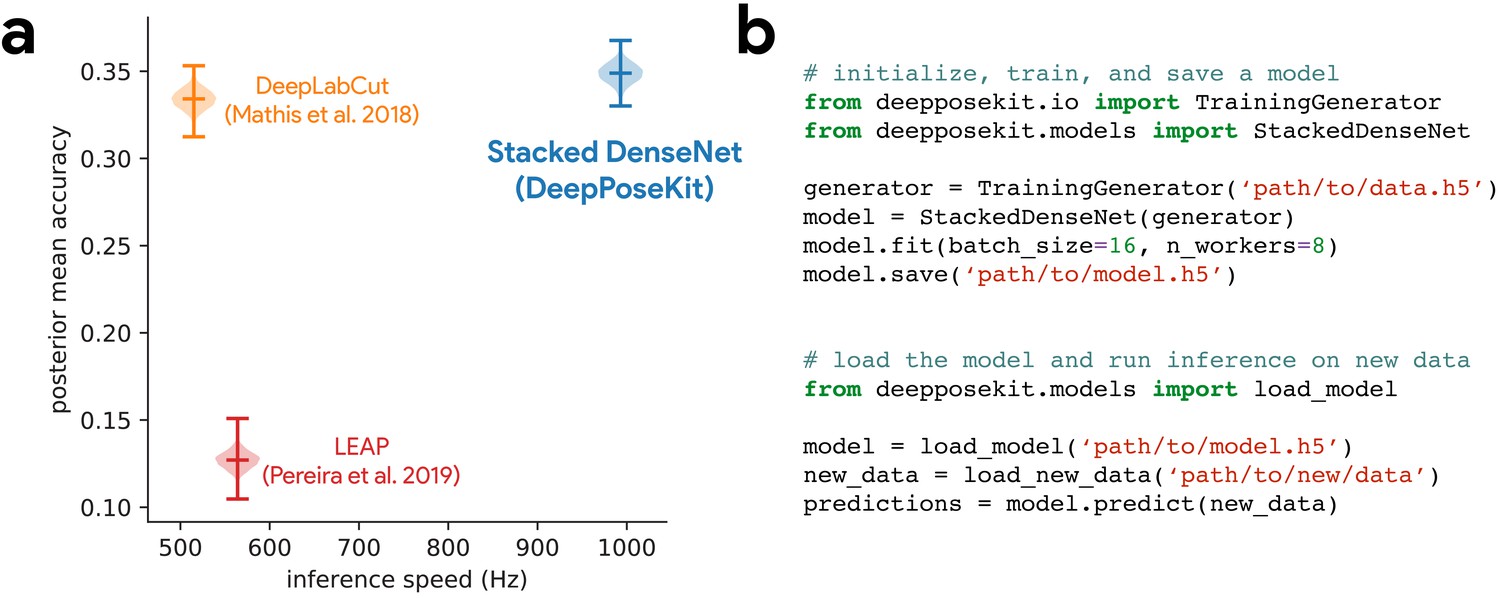
DeepPoseKit is fast, accurate, and easy-to-use.
Our Stacked DenseNet model estimates posture at approximately 2×—or greater—the speed of the LEAP model (Pereira et al., 2019) and the DeepLabCut model (Mathis et al., 2018) while also achieving similar accuracy to the DeepLabCut model (Mathis et al., 2018)—shown here as mean accuracy for our most challenging dataset of multiple interacting Grévy’s zebras (E. grevyi) recorded in the wild (a). See Figure 3—figure supplement 1 for further details. Our software interface is designed to be straightforward but flexible. We include many options for expert users to customize model training with sensible default settings to make pose estimation as easy as possible for beginners. For example, training a model and running inference on new data requires writing only a few lines of code and specifying some basic settings (b).
Figure 3—figure supplement 1
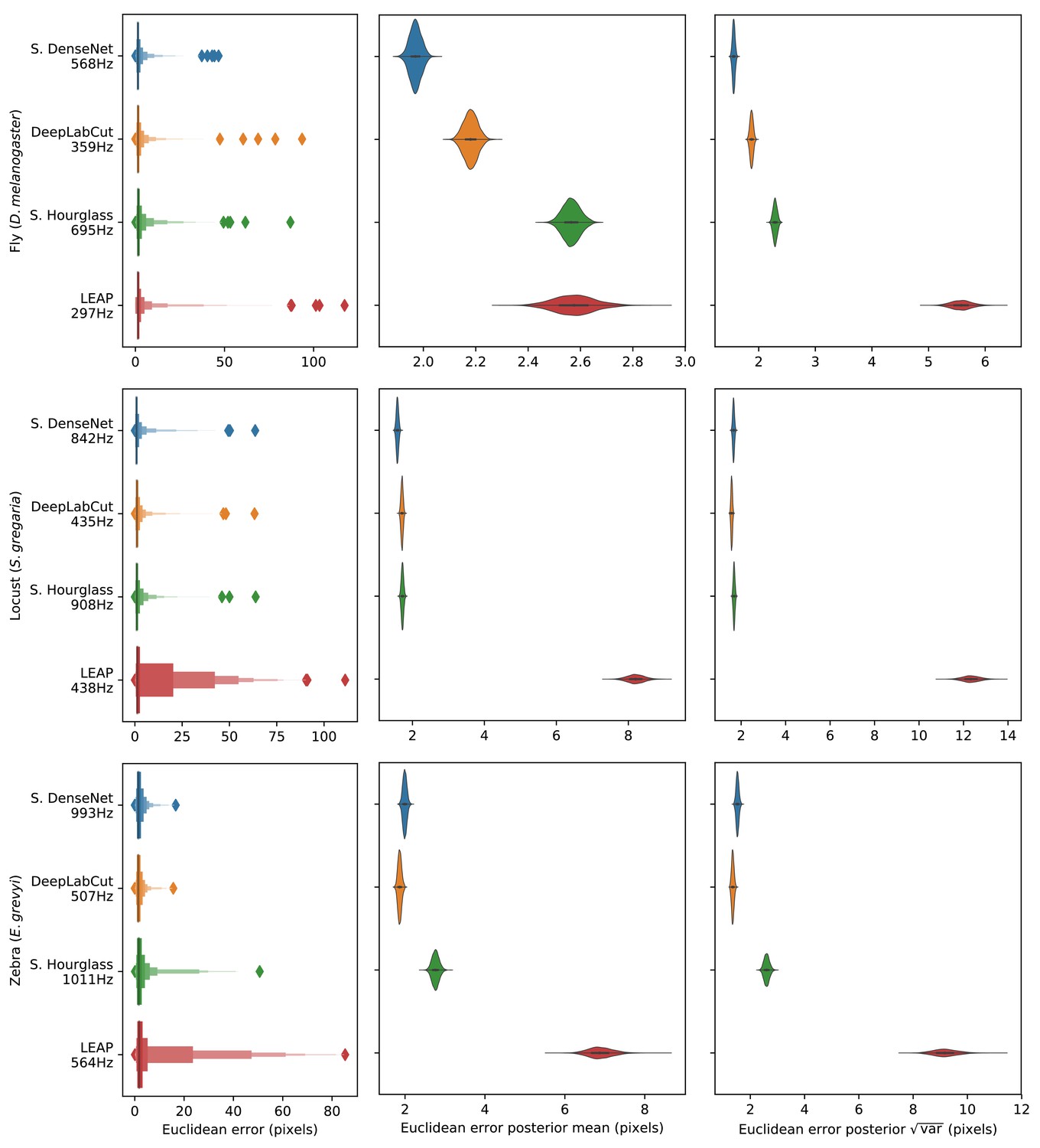
Euclidean error distributions for each model across our three datasets.
Letter-value plots (left) show the raw error distributions for each model. Violinplots of the posterior distributions for the mean and variance (right) show statistical differences between the error distributions. Overall the LEAP model (Pereira et al., 2019) was the worst performer on every dataset in terms of both mean and variance. Our Stacked DenseNet model was the best performer for the fly dataset, while our Stacked DenseNet model and the DeepLabCut model (Mathis et al., 2018) both performed equally well on the locust and zebra datasets. The posteriors for the DeepLabCut model (Mathis et al., 2018) and our Stacked DenseNet model are highly overlapping for these datasets, which suggests they are not statistically discernible from one another. Our Stacked Hourglass model (Newell et al., 2016) performed equally to the DeepLabCut model (Mathis et al., 2018) and our Stacked DenseNet model for the locust dataset but performed slightly worse for the fly and zebra datasets.
Figure 4 with 3 supplements
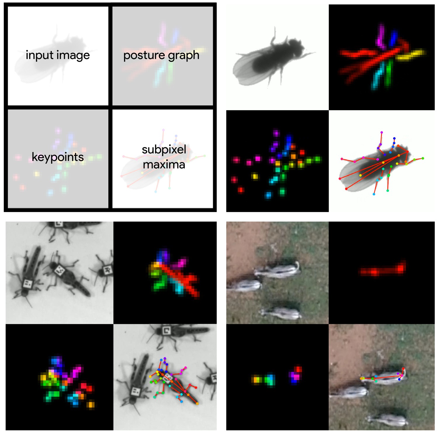
Datasets used for evaluation.
A visualization of the datasets we used to evaluate our methods (Table 1). For each dataset, confidence maps for the keypoints (bottom-left) and posture graph (top-right) are illustrated using different colors for each map. These outputs are from our Stacked DenseNet model at resolution.
Figure 4—video 1
A video of a behaving fly from Pereira et al. (2019) with pose estimation outputs visualized.
Figure 4—video 2
A video of a behaving locust with pose estimation outputs visualized.
Figure 4—video 3
A video of a behaving Grévy’s zebra with pose estimation outputs visualized.
Appendix 1—figure 1
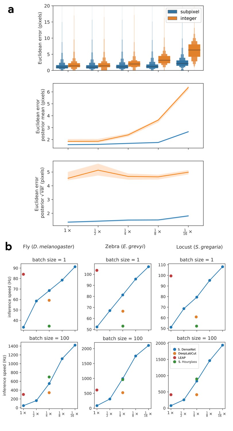
Our subpixel maxima algorithm increases speed without decreasing accuracy.
Prediction accuracy on the fly dataset is maintained across downsampling configurations (a). Letter-value plots (a-top) show the raw error distributions for each configuration. Visualizations of the credible intervals (99% highest-density region) of the posterior distributions for the mean and variance (a-bottom) illustrate statistical differences between the error distributions, where using subpixel maxima decreases both the mean and variance of the error distribution. Inference speed is fast and can be run in real-time on single images (batch size = 1) at ~30–110 Hz or offline (batch size = 100) upwards of 1000 Hz (b). Plots show the inference speeds for our Stacked DenseNet model across downsampling configurations as well as the other models we tested for each of our datasets.
-
Appendix 1—figure 1—source data 1
Raw prediction errors for experiments in Appendix 1—figure 1a.
See 'Materials and methods’ for details.
- https://cdn.elifesciences.org/articles/47994/elife-47994-app1-fig1-data1-v2.csv
Appendix 1—figure 2
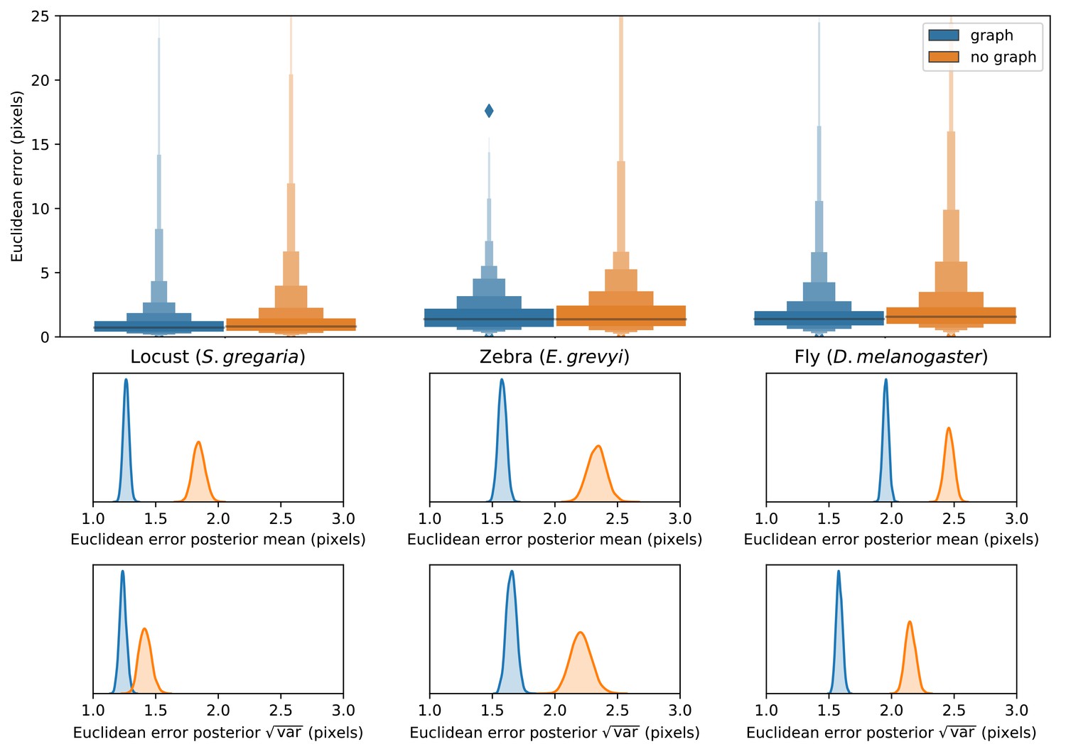
Predicting the multi-scale geometry of the posture graph reduces error.
Letter-value plots (top) show the raw error distributions for each experiment. Visualizations of the posterior distributions for the mean and variance (bottom) show statistical differences between the error distributions. Predicting the posture graph decreases both the mean and variance of the error distribution.
-
Appendix 1—figure 2—source data 1
Raw prediction errors for experiments in Appendix 1—figure 2.
See 'Materials and methods’ for details.
- https://cdn.elifesciences.org/articles/47994/elife-47994-app1-fig2-data1-v2.csv
Appendix 1—figure 3
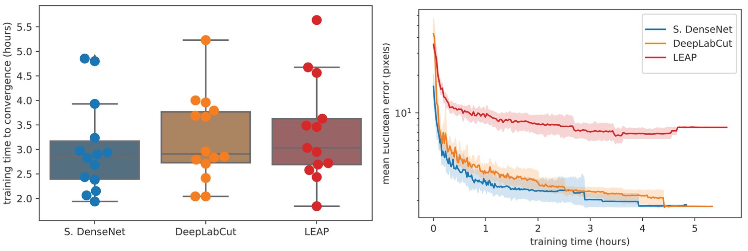
Training time required for our Stacked DenseNet model, the DeepLabCut model (Mathis et al., 2018), and the LEAP model (Pereira et al., 2019) (n = 15 per model) using our zebra dataset.
Boxplots and swarm plots (left) show the total training time to convergence (<0.001 improvement in validation loss for 50 epochs). Line plots (right) illustrate the Euclidean error of the validation set during training, where error bars show bootstrapped (n = 1000) 99% confidence intervals of the mean. Fully training models to convergence requires only a few hours of optimization (left) with reasonable accuracy reached after only 1 hr (right) for our Stacked DenseNet model.
-
Appendix 1—figure 3—source data 1
Total training time for each model in Appendix 1—figure 3.
- https://cdn.elifesciences.org/articles/47994/elife-47994-app1-fig3-data1-v2.csv
-
Appendix 1—figure 3—source data 2
Mean euclidean error as a function of training time for each model in Appendix 1—figure 3.
- https://cdn.elifesciences.org/articles/47994/elife-47994-app1-fig3-data2-v2.csv
Appendix 1—figure 4
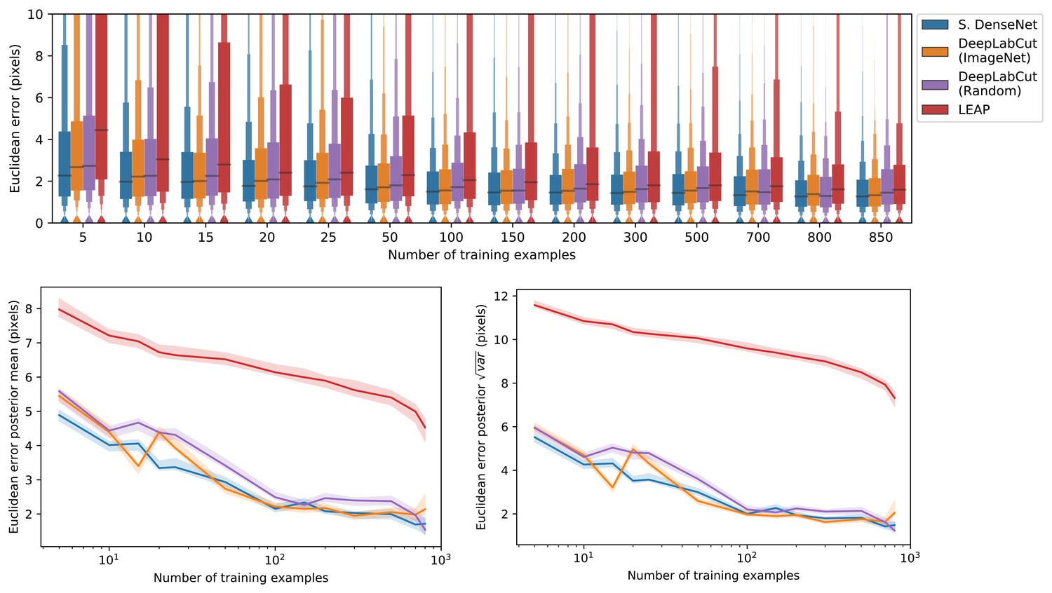
A comparison of prediction accuracy with different numbers of training examples from our zebra dataset.
The error distributions shown as letter-value plots (top) illustrate the Euclidean error for the remainder of the dataset not used for training—with a total of 900 labeled examples in the dataset. Line plots (bottom) show posterior credible intervals (99% highest-density region) for the mean and variance of the error distributions. We tested our Stacked DenseNet model; the DeepLabCut model (Mathis et al., 2018) with transfer learning—that is with weights pretrained on ImageNet (Deng et al., 2009); the same model without transfer learning—that is with randomly-initialized weights; and the LEAP model (Pereira et al., 2019). Our Stacked DenseNet model achieves high accuracy using few training examples without the use the transfer learning. Using pretrained weights does slightly decrease overall prediction error for the DeepLabCut model (Mathis et al., 2018), but the effect size is relatively small.
-
Appendix 1—figure 4—source data 1
Raw prediction errors for experiments in Appendix 1—figure 4.
See 'Materials and methods’ for details.
- https://cdn.elifesciences.org/articles/47994/elife-47994-app1-fig4-data1-v2.csv
Appendix 4—figure 1
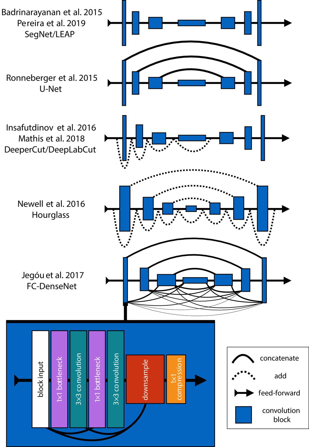
An illustration showing the progression of encoder-decoder architectures from the literature—ordered by performance from top to bottom (see Appendix 4: 'Encoder-decoder models' for further details).
Most advances in performance have come from adding connections between layers in the network, culminating in FC-DenseNet from Jégou et al. (2017). Lines in each illustration indicate connections between convolutional blocks with the thickness of the line indicating the magnitude of information flow between layers in the network. The size of each convolution block indicates the relative number of feature maps (width) and spatial scale (height). The callout for FC-DenseNet (Jégou et al., 2017; bottom-left) shows the elaborate set of skip connections within each densely-connected convolutional block as well as our additions of bottleneck and compression layers (described by Huang et al., 2017a) to increase efficiency (Appendix 8).
Appendix 4—figure 2
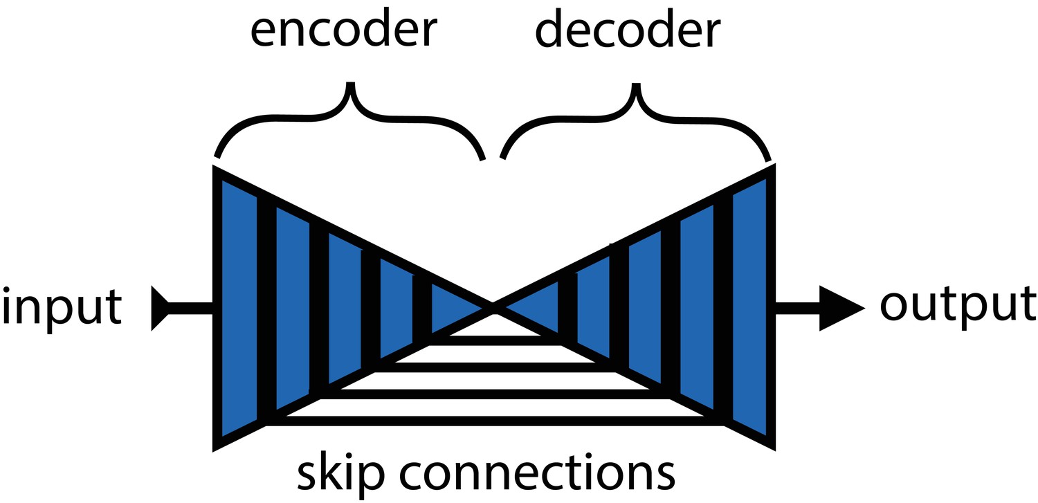
An illustration of the basic encoder-decoder design.
The encoder converts the input images into spatial features, and the decoder transforms spatial features to the desired output.
Appendix 8—figure 1 with 3 supplements
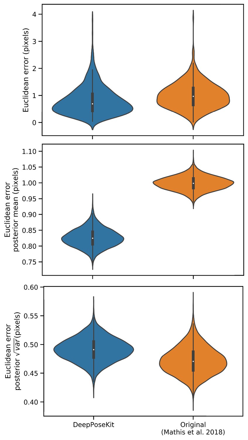
Prediction errors for the odor-trail mouse dataset from Mathis et al. (2018) using the original implementation of the DeepLabCut model (Mathis et al., 2018; Nath et al., 2019) and our modified version of this model implemented in DeepPoseKit.
Mean prediction error is slightly lower for the DeepPoseKit implementation, but there is no discernible difference in variance. These results indicate that the models achieve nearly identical prediction accuracy despite modification. We also provide qualitative comparisons of these results in Appendix 8—figure 1—figure supplement 1 and 2, and Appendix 8—figure 1—video 1.
-
Appendix 8—figure 1—source data 1
Raw prediction errors for our DeepLabCut model (Mathis et al., 2018) reimplemented in DeepPoseKit in Appendix 8—figure 1.
See 'Materials and methods’ for details.
- https://cdn.elifesciences.org/articles/47994/elife-47994-app8-fig1-data1-v2.csv
-
Appendix 8—figure 1—source data 2
Raw prediction errors for the original DeepLabCut model from Mathis et al. (2018) in Appendix 8—figure 1.
See 'Materials and methods’ for details.
- https://cdn.elifesciences.org/articles/47994/elife-47994-app8-fig1-data2-v2.csv
Appendix 8—figure 1—video 1
A video comparison of the tracking output of our implementation of the DeepLabCut model (Mathis et al., 2018) in DeepPoseKit vs. the original implementation from Mathis et al. (2018) and Nath et al. (2019).
Appendix 8—figure 1—figure supplement 1
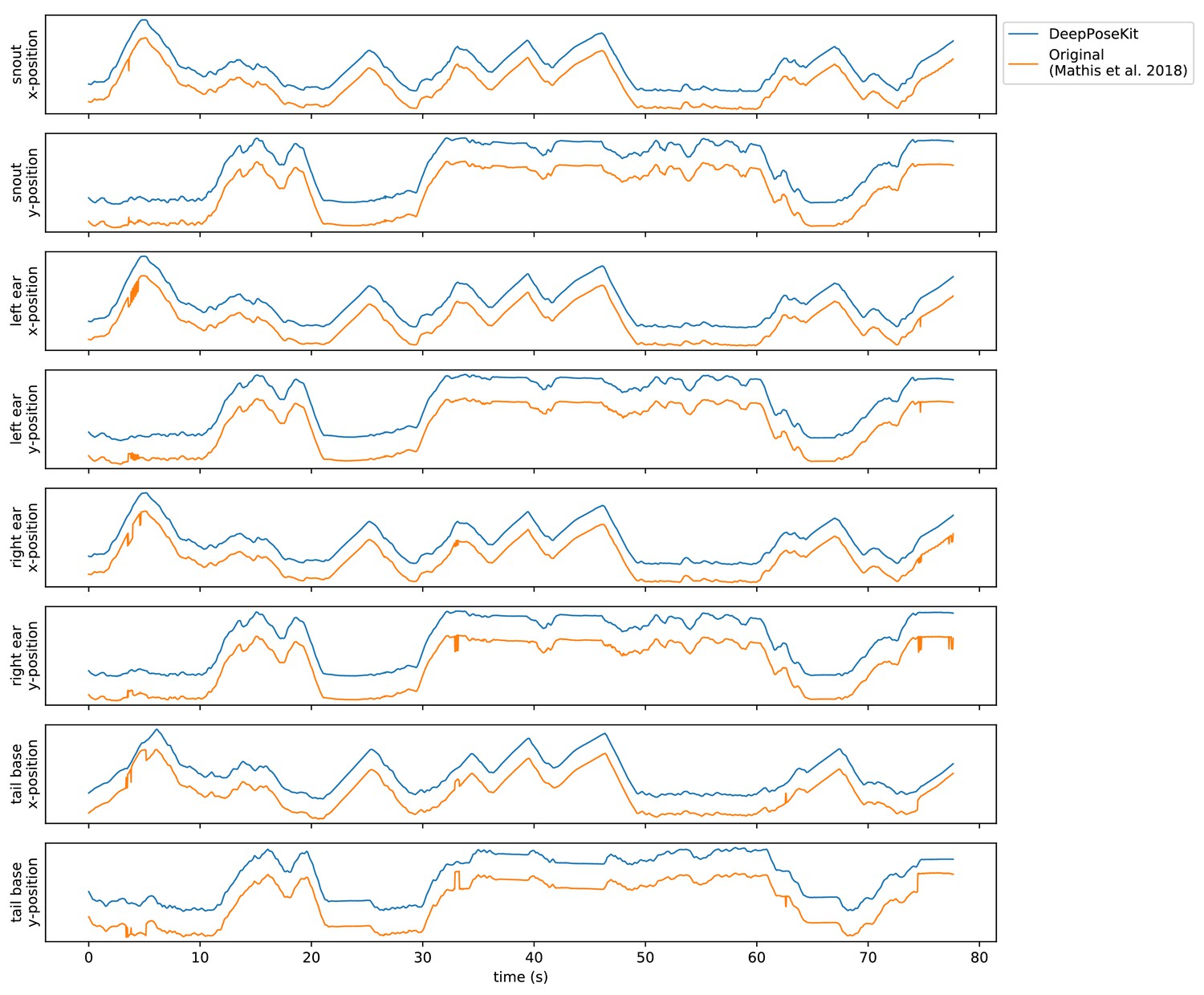
Plots of the predicted output for Appendix 8—figure 1—video 1 comparing our implementation of the DeepLabCut model (Mathis et al., 2018) in DeepPoseKit vs. the original implementation from Mathis et al. (2018), and Nath et al. (2019).
Note the many fast jumps in position for the original verison from Mathis et al. (2018), which indicates prediction errors.
Appendix 8—figure 1—figure supplement 2
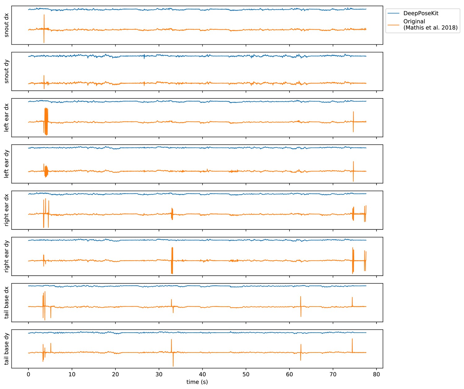
Plots of the temporal derivatives of the predicted output for Appendix 8—figure 1—video 1 comparing our implementation of the DeepLabCut model (Mathis et al., 2018) in DeepPoseKit vs. the original implementation from Mathis et al. (2018), and Nath et al. (2019).
Note the many fast jumps in position for the original verison from Mathis et al. (2018), which indicates prediction errors.
Tables
Table 1
Datasets used for model comparisons.
| Name | Species | Resolution | # Images | # Keypoints | Individuals | Source |
|---|---|---|---|---|---|---|
| Vinegar fly | Drosophila melanogaster | 192 × 192 | 1500 | 32 | Single | Pereira et al., 2019 |
| Desert locust | Schistocerca gregaria | 160 × 160 | 800 | 35 | Multiple | This paper |
| Grévy’s zebra | Equus grevyi | 160 × 160 | 900 | 9 | Multiple | This paper |
Additional files
-
Transparent reporting form
- https://cdn.elifesciences.org/articles/47994/elife-47994-transrepform-v2.docx
-
Appendix 1—figure 1—source data 1
Raw prediction errors for experiments in Appendix 1—figure 1a.
See 'Materials and methods’ for details.
- https://cdn.elifesciences.org/articles/47994/elife-47994-app1-fig1-data1-v2.csv
-
Appendix 1—figure 2—source data 1
Raw prediction errors for experiments in Appendix 1—figure 2.
See 'Materials and methods’ for details.
- https://cdn.elifesciences.org/articles/47994/elife-47994-app1-fig2-data1-v2.csv
-
Appendix 1—figure 3—source data 1
Total training time for each model in Appendix 1—figure 3.
- https://cdn.elifesciences.org/articles/47994/elife-47994-app1-fig3-data1-v2.csv
-
Appendix 1—figure 3—source data 2
Mean euclidean error as a function of training time for each model in Appendix 1—figure 3.
- https://cdn.elifesciences.org/articles/47994/elife-47994-app1-fig3-data2-v2.csv
-
Appendix 1—figure 4—source data 1
Raw prediction errors for experiments in Appendix 1—figure 4.
See 'Materials and methods’ for details.
- https://cdn.elifesciences.org/articles/47994/elife-47994-app1-fig4-data1-v2.csv
-
Appendix 8—figure 1—source data 1
Raw prediction errors for our DeepLabCut model (Mathis et al., 2018) reimplemented in DeepPoseKit in Appendix 8—figure 1.
See 'Materials and methods’ for details.
- https://cdn.elifesciences.org/articles/47994/elife-47994-app8-fig1-data1-v2.csv
-
Appendix 8—figure 1—source data 2
Raw prediction errors for the original DeepLabCut model from Mathis et al. (2018) in Appendix 8—figure 1.
See 'Materials and methods’ for details.
- https://cdn.elifesciences.org/articles/47994/elife-47994-app8-fig1-data2-v2.csv
Download links
A two-part list of links to download the article, or parts of the article, in various formats.
Downloads (link to download the article as PDF)
Open citations (links to open the citations from this article in various online reference manager services)
Cite this article (links to download the citations from this article in formats compatible with various reference manager tools)
DeepPoseKit, a software toolkit for fast and robust animal pose estimation using deep learning
eLife 8:e47994.
https://doi.org/10.7554/eLife.47994


