A neural mechanism for contextualizing fragmented inputs during naturalistic vision
- University of York, United Kingdom
- Freie Universität Berlin, Germany
- Goethe-Universität Frankfurt, Germany
- Humboldt-Universität Berlin, Germany
- Bernstein Center for Computational Neuroscience Berlin, Germany
Figures
Figure 1 with 1 supplement
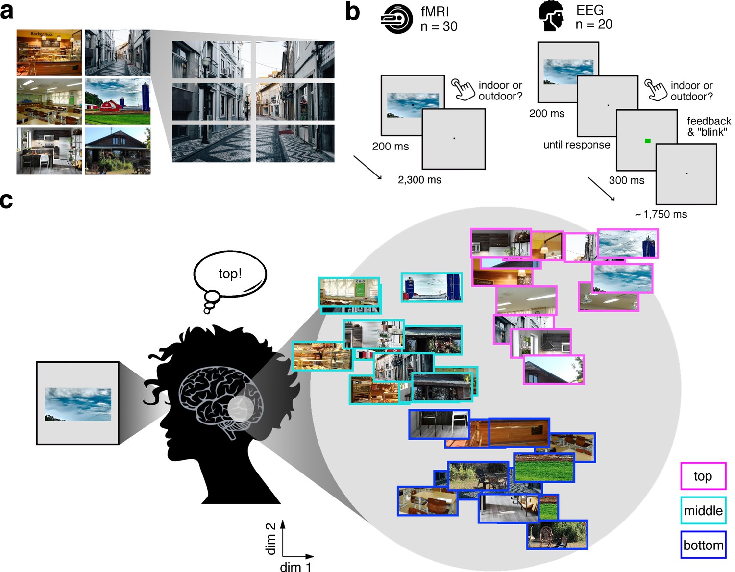
Experimental design and rationale of schema-based information sorting.
(a) The stimulus set consisted of six natural scenes (three indoor, three outdoor). Each scene was split into six rectangular fragments. (b) During the fMRI and EEG recordings, participants performed an indoor/outdoor categorization task on individual fragments. Notably, all fragments were presented at central fixation, removing explicit location information. (c) We hypothesized that the visual system sorts sensory input by spatial schemata, resulting in a cortical organization that is explained by the fragments’ within-scene location, predominantly in the vertical dimension: Fragments stemming from the same part of the scene should be represented similarly. Here we illustrate the hypothesized sorting in a two-dimensional space. A similar organization was observed in multi-dimensional scaling solutions for the fragments’ neural similarities (see Figure 1—figure supplement 1 and Video 1). In subsequent analyses, the spatiotemporal emergence of the schema-based cortical organization was precisely quantified using representational similarity analysis (Figure 2).
Figure 1—figure supplement 1
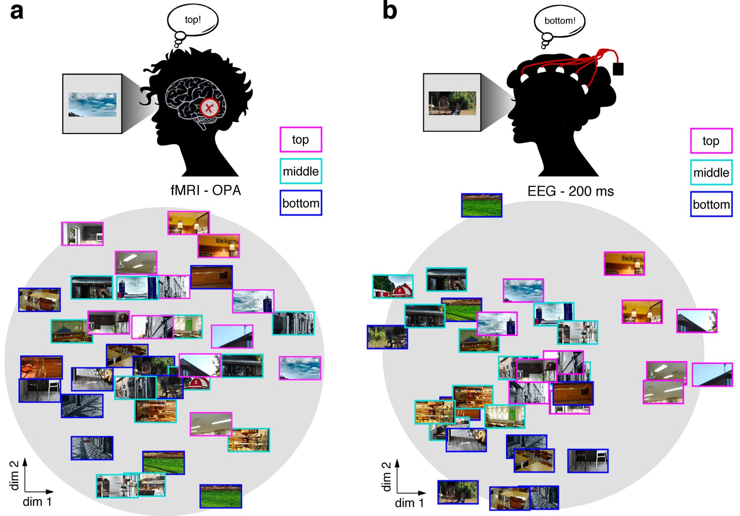
MDS visualization of neural RDMs 34 MDS visualization of neural RDMs.
(a/b) A multi-dimensional scaling (MDS) of the fragments’ neural similarity in OPA (a) and after 200 ms of processing (b) revealed a sorting according to vertical location, which was visible in a two-dimensional solution. This visualization suggests that schemata are a prominent organizing principle for representations in OPA and after 200 ms of vision. A time-resolved MDS for the EEG data can be found in Video 1.
Figure 2 with 9 supplements
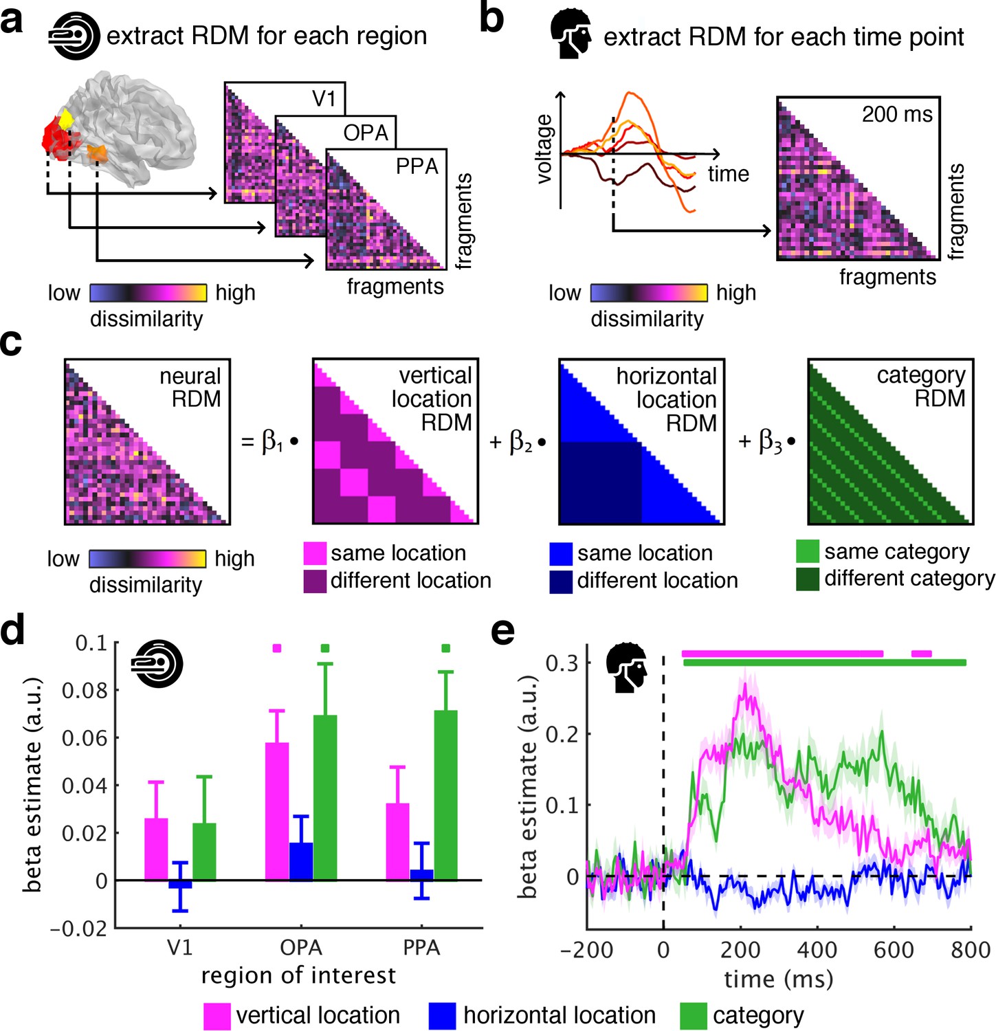
Spatial schemata determine cortical representations of fragmented scenes.
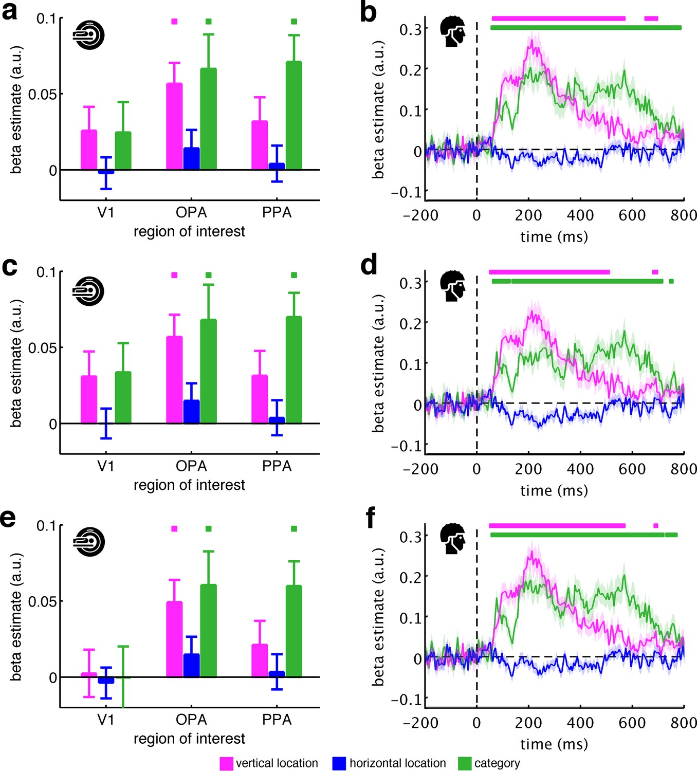
(a) To test where and when the visual system sorts incoming sensory information by spatial schemata, we first extracted spatially (fMRI) and temporally (EEG) resolved neural representational dissimilarity matrices (RDMs). In the fMRI, we extracted pairwise neural dissimilarities of the fragments from response patterns across voxels in the occipital place area (OPA), parahippocampal place area (PPA), and early visual cortex (V1). (b) In the EEG, we extracted pairwise dissimilarities from response patterns across electrodes at every time point from −200 ms to 800 ms with respect to stimulus onset. (c) We modelled the neural RDMs with three predictor matrices, which reflected their vertical and horizontal positions within the full scene, and their category (i.e., their scene or origin). (d) The fMRI data revealed a vertical-location organization in OPA, but not V1 and PPA. Additionally, the fragment’s category predicted responses in both scene-selective regions. (e) The EEG data showed that both vertical location and category predicted cortical responses rapidly, starting from around 100 ms. These results suggest that the fragments’ vertical position within the scene schema determines rapidly emerging representations in scene-selective occipital cortex. Significance markers represent p<0.05 (corrected for multiple comparisons). Error margins reflect standard errors of the mean. In further analysis, we probed the flexibility of this schematic coding mechanism (Figure 3).
Figure 2—figure supplement 1
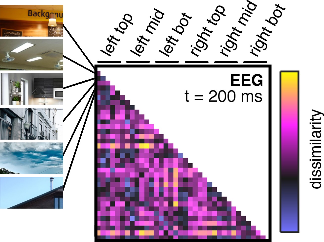
Details on neural dissimilarity construction.
Pairwise neural dissimilarity values were into representational dissimilarity matrices (RDMs), so that for every time point one 36 × 36 matrix containing estimates of neural dissimilarity was available. Here, an example RDM at 200 ms post-stimulus is shown, which exemplifies the ordering of fragment combinations for all RDMs.
Figure 2—figure supplement 2
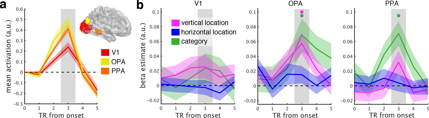
fMRI response time courses.
(a) Functional MRI data were analyzed in three regions of interest (here shown on the right hemisphere): primary visual cortex (V1), occipital place area (OPA), and parahippocampal place area (PPA). Each of these ROIs showed reliable net responses to the fragments, peaking 3 TRs after stimulus onset. The activation time courses were baseline-corrected by subtracting the activation from the first two TRs. (b), GLM analysis across the response time course. Most prominently after 3 TRs, the neural organization in OPA was explained by the fragments’ vertical location, reflecting a neural coding in accordance with spatial schemata. Additionally, scene category predicted neural organization in OPA and PPA. Error margins reflect standard errors of the mean. Significance markers represent p<0.05 (corrected for multiple comparisons across ROIs).
Figure 2—figure supplement 3

Pairwise decoding across EEG electrode groups.
Based on previous studies on multivariate decoding of visual information, we restricted our main analysis to a group of posterior electrodes (where we expected the strongest effects). For comparison, we also analyzed data in central and anterior electrode groups. The central group consisted of 20 electrodes (C3, TP9, CP5, CP1, TP10, CP6, CP2, Cz, C4, C1, C5, TP7, CP3, CPz, CP4, TP8, (C6, C2, T7, T8) and the anterior group consisted of 26 electrodes (F3, F7, FT9, FC5, FC1, FT10, FC6, FC2, F4, F8, Fp2, AF7, AF3, AFz, F1, F5, FT7, FC3, FCz, FC4, FT8, F6, F2, AF4, AF8, Fpz). RDMs were constructed in an identical fashion to the posterior group used for the main analyses (Figure 2—figure supplement 1). We computed general discriminability of the 36 scene fragments in the three groups by averaging all off-diagonal elements of the RDMs. As expected, the resulting time courses of pair-wise discriminability revealed the strongest overall decoding in the posterior group, followed by the central and anterior groups. RSA results for these electrodes are found in Figure 2—figure supplement 4/5. Significance markers represent p<0.05 (corrected for multiple comparisons). Error margins reflect standard errors of the mean.
Figure 2—figure supplement 4
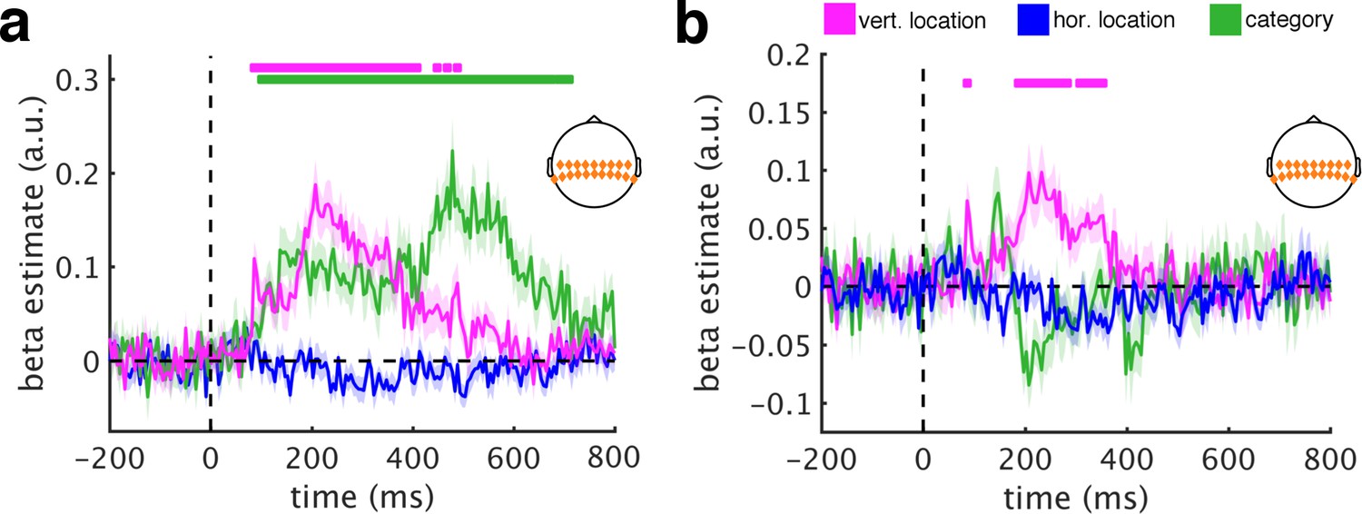
RSA using central electrodes.
(a/b) Repeating the main RSAs for the central electrode group yielded a similar pattern as the posterior group, revealing both vertical location information (from 85 ms to 485 ms) and category information (from 100 ms to 705 ms). (c/d) Removing DNN features abolished category information, but not vertical location information, most prominently between 185 ms and 350 ms. This result is consistent with the schematic coding observed for posterior signals. Significance markers represent p<0.05 (corrected for multiple comparisons). Error margins reflect standard errors of the mean.
Figure 2—figure supplement 5

RSA using anterior electrodes.
(a/b) Also responses recorded from the anterior group yielded both vertical location information (from 85 ms to 350 ms) and category information (from 165 ms to 610 ms). (c/d) In contrast to the other electrode groups, removing DNN features rendered location and category information insignificant, suggesting that they are not primarily linked to sources in frontal brain areas. This observation also excludes explanations based on oculomotor confounds. Significance markers represent p<0.05 (corrected for multiple comparisons). Error margins reflect standard errors of the mean.
Figure 2—figure supplement 6

Vertical location effects across experiment halves.
We interpret the vertical location organization in the neural data as reflecting prior schematic knowledge about scene structure. Alternatively, however, the vertical location organization could in principle result from learning the composition of the scenes across the experiment. In the latter case, one would predict that vertical location effects should primarily occur late in the experiment (e.g., in the second half), and less so towards the beginning (e.g., in the first half). To test this, we split into halves both the fMRI data (three runs each) and the EEG data (first versus second half of trials) and for each half modeled the neural data as a function of the vertical and horizontal location and category predictors. (a) For the fMRI data, we found significant vertical location information in the OPA for in the first half (t[29]=3.46, p<0.001, pcorr <0.05) and a trending effect for the second half (t[29] = 2.07, p = 0.024, pcorr >0.05). No differences between the splits were found in any region (all t<0.90, p>0.37). (b) For the EEG data, we also found very similar results for the two spits, with no significant differences emerging at any time point. Together, these results suggest that the vertical location organization cannot solely be explained by extensive learning over the course of the experiment. Significance markers represent p<0.05 (corrected for multiple comparisons). Empty markers represent p<0.05 (uncorrected). Error margins reflect standard errors of the mean.
Figure 2—figure supplement 7
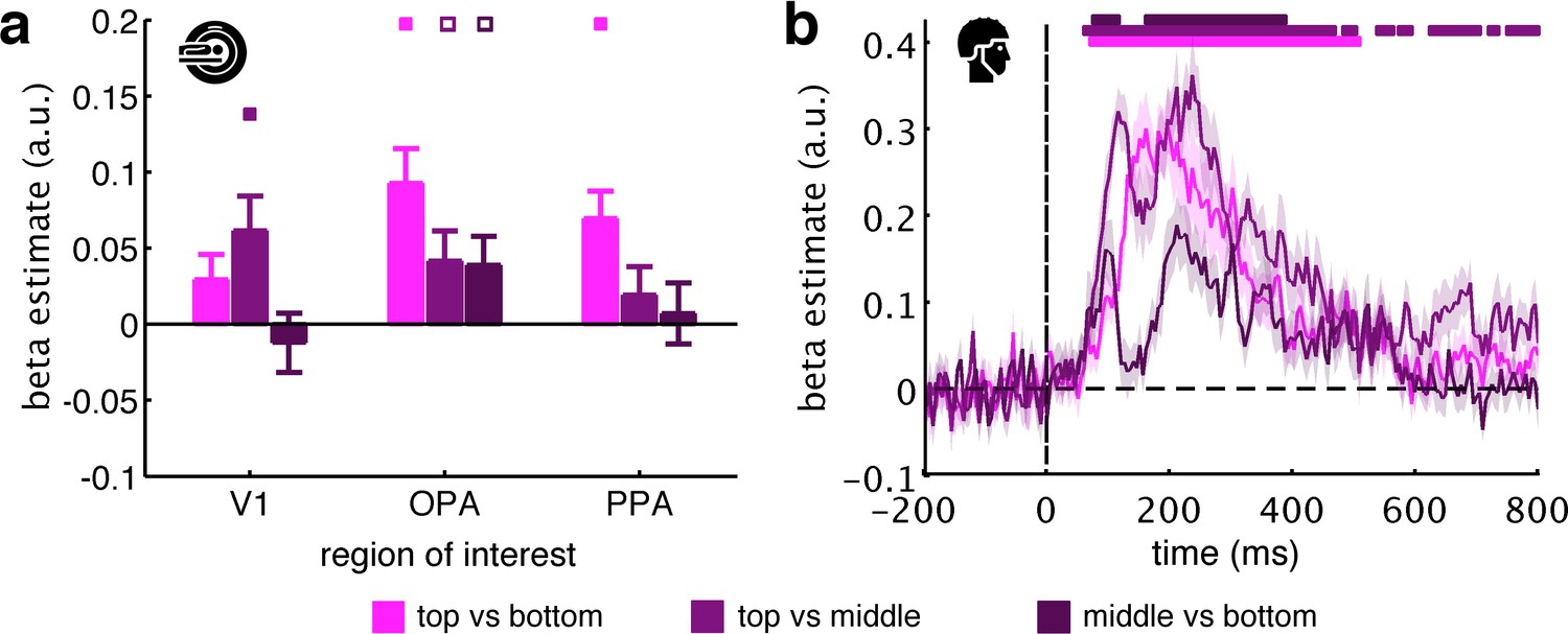
Pairwise comparisons along the vertical axis.
To test whether vertical location information can be observed across all three vertical bins, we modelled the neural data as a function of the fragments’ vertical location, now separately for each pairwise comparison along the vertical axis (i.e., top versus bottom, top versus middle, and middle versus bottom). (a) For the fMRI data, we only found consistent evidence for vertical location information in the OPA: top versus bottom (t[29]=4.10, p<0.001, pcorr <0.05), top versus middle (t[29]=2.13, p=0.021, pcorr >0.05), middle versus bottom (t[29]=2.06, p=0.024, pcorr >0.05). Although the effect was numerically bigger for top versus bottom, we did not find a significant difference between the three pairwise comparisons in OPA (F[2,58]=2.71, p=0.075). (b) For the EEG data, we found significant vertical location information for all three comparisons. Here, the middle-versus-bottom comparison yielded the weakest effect, which was significantly smaller than the effect for top versus bottom from 120 ms and 195 ms and significantly smaller than the effect for top versus middle from 110 ms to 285 ms. Together, these results suggest that schematic coding can be observed consistently across the different comparisons along the vertical axis, although comparisons including the top fragments yielded stronger effects. Significance markers represent p<0.05 (corrected for multiple comparisons). Empty markers represent p<0.05 (uncorrected). Error margins reflect standard errors of the mean.
Figure 2—figure supplement 8
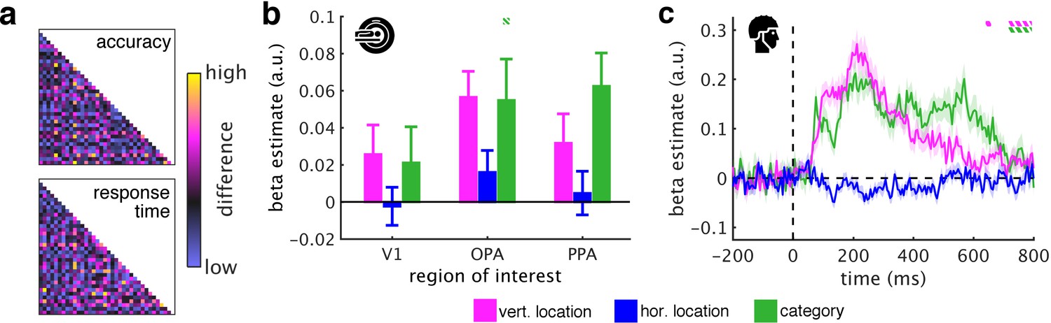
Controlling for task difficulty.
(a) To control for task difficulty effects in the indoor/outdoor classification task, we computed paired t-tests between all pairs of fragments, separately for their associated accuracies and response times. We then constructed two predictor RDMs that contained the t-values of the pairwise tests between the fragments: For each pair of fragments, these t-values corresponded to dissimilarity in task difficulty (e.g., comparing two fragments associated with similarly short categorization response times would yield a low t-value, and thus low dissimilarity). This was done separately for the fMRI and EEG experiments (matrices from the EEG experiment are shown). The accuracy and response time RDMs were mildly correlated with the category RDM (fMRI: accuracy: r = 0.10, response time: r = 0.15; EEG: accuracy: r = 0.17, response time: r = 0.16), but not with the vertical location RDM (fMRI: both r < 0.01, EEG: both r < 0.01). After regressing out the task difficulty RDMs, we found highly similar vertical location and category information as in the previous analyses (Figure 3b/c). (b) In the fMRI, only category information in OPA was significantly reduced when task difficulty was accounted for. (c) In the EEG, towards the end of the epoch – when participants responded – location and category information were decreased. This shows that the effects of schematic coding – emerging around 200 ms after onset – cannot be explained by differences in task difficulty. The dashed significance markers represent significantly reduced information (compared to the main analyses, Figure 3b/c) at p<0.05 (corrected for multiple comparisons).
Figure 2—figure supplement 9
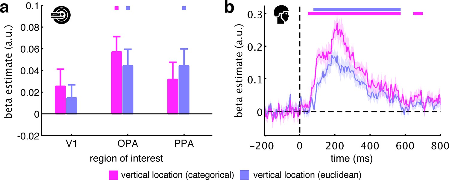
Categorical versus Euclidean vertical location predictors.
We defined our vertical location predictor as categorical, assuming that top, middle, and bottom fragments are coded distinctly in the human brain. An alternative way of constructing the vertical location predictor is in terms of the fragments’ Euclidean distances, where fragments closer together along the vertical axis (e.g., top and middle) are represented more similarly than fragments further apart (e.g., top and bottom). (a) For the fMRI data, we found that the categorical and Euclidean predictors similarly explained the neural data, with no statistical differences between them (all t[29] <1.15, p>0.26). (b) For the EEG data, we found that both predictors explained the neural data well. However, the categorical predictor revealed significantly stronger vertical location information from 75 ms to 340 ms, suggesting that, at least in the EEG data, the differentiation along the vertical axis is more categorical in nature. Significance markers represent p<0.05 (corrected for multiple comparisons). Error margins reflect standard errors of the mean.
Figure 3 with 3 supplements

Schematic coding operates flexibly across visual and conceptual scene properties.
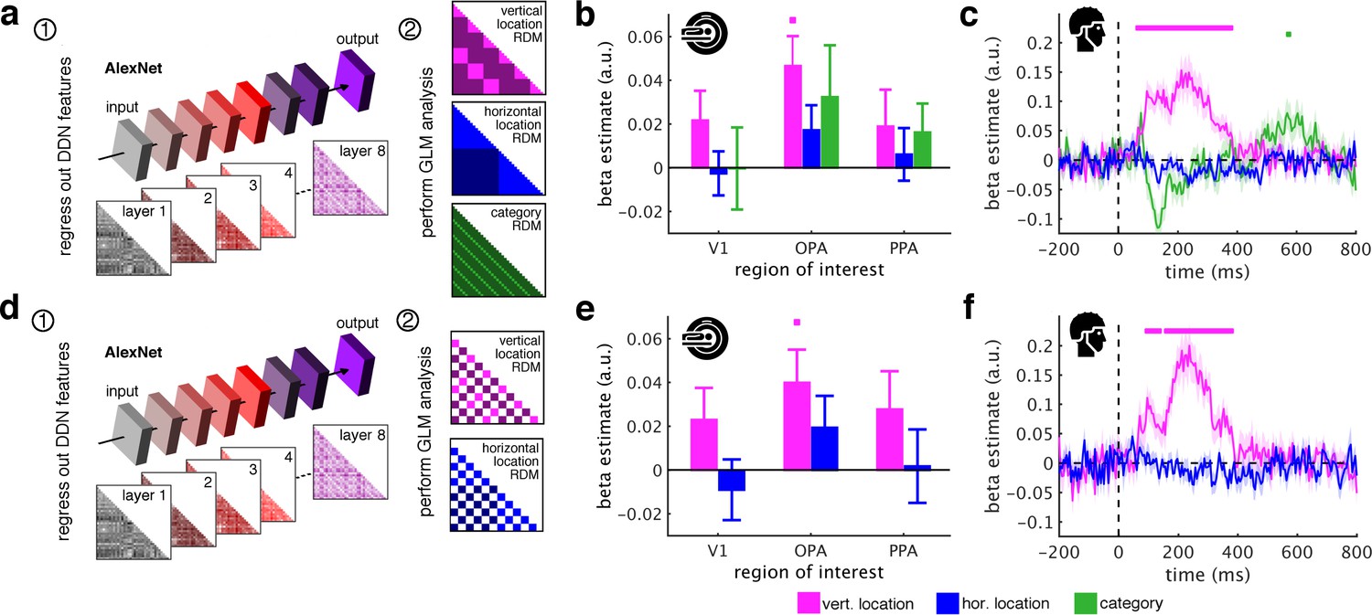
(a) To determine the role of categorization-related visual features in this schematic organization, we regressed out RDMs obtained from 18 layers along the ResNet50 DNN before repeated the three-predictor general linear model (GLM) analysis (Figure 2c). (b/c) Removing DNN features abolished category information in fMRI and EEG signals, but not vertical location information. (d) To test for generalization across different scene types, we restricted location predictor RDMs to comparisons across indoor and outdoor scenes. Due to this restriction, category could not be modelled. (e/f) In this analysis, vertical location still predicted neural organization in OPA and from 70 ms. (g) Finally, we combined the two analyses: we first regressed out DNN features prior and then modelled the neural RDMs using the restricted predictor RDMs (d). (h) In this analysis, we still found significant vertical location information in OPA. (i) Notably, vertical location information in the EEG signals was delayed to after 180 ms, suggesting that at this stage schematic coding becomes flexible to visual and conceptual attributes. Significance markers represent p<0.05 (corrected for multiple comparisons). Error margins reflect standard errors of the mean.
Figure 3—figure supplement 1
AlexNet as a model of visual categorization.
(a) In addition to the ResNet50 DNN, we also used the more widely used AlexNet DNN architecture (pretrained on the ImageNet dataset, implemented in the MatConvNet toolbox) as a model for visual categorization. AlexNet consists of 5 convolutional and three fully-connected layers. We created 8 RDMs, separately for each layer of the DNN. (b/c) Removing the AlexNet DNN features rendered category information non-significant in fMRI and EEG signals. However, we still found vertical location information in OPA and from 65 ms to 375 ms. (c–e) When additionally restricting the analysis to comparisons between indoor and outdoor scenes, the fragments’ vertical location still predicted neural activations in OPA and from 95 ms to 375 ms. In sum, these results are highly similar to the results obtained with the ResNet50 model (Figure 3b/c/h/i). Significance markers represent p<0.05 (corrected for multiple comparisons). Error margins reflect standard errors of the mean.
Figure 3—figure supplement 2
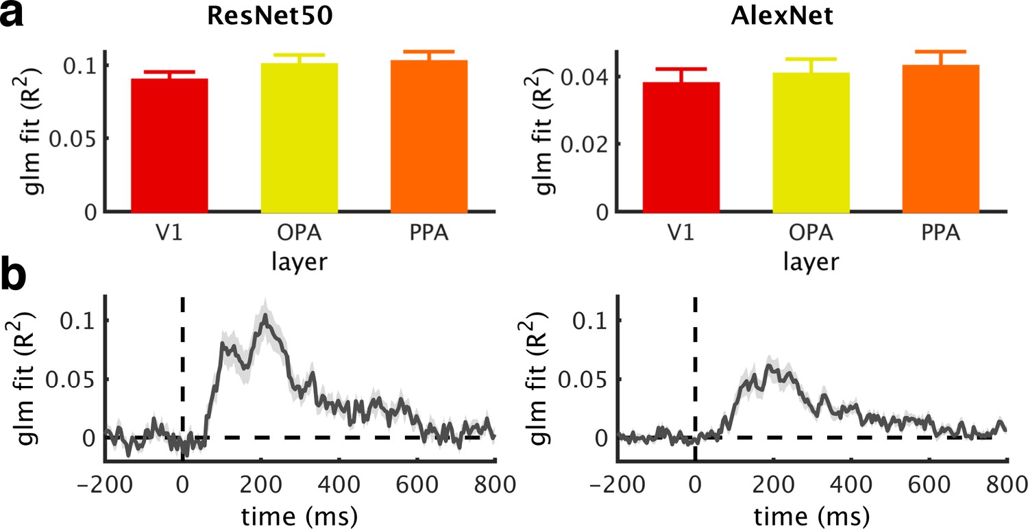
DNN model fit.
(a/b) Goodness of fit (R2) across ROIs (a) and time (b) of the GLMs used to regress out DNN features, obtained from ResNet50 (left) or AlexNet (right). For the EEG time series, mean R2 across the baseline period were subtracted. Note that GLMs based on the ResNet50 RDMs had more predictor variables, which may contribute to their better fit. Error bars represent standard errors of the mean.
Figure 3—figure supplement 3
Low-level control models.
We used three control models that explicitly account for low-level visual features: a pixel-dissimilarity model, GIST descriptors, and the fragments’ neural dissimilarity in V1. Critically, all three models did not account for the fragments’ vertical location organization. Moreover, unlike the DNN models, the low-level models were also unable to account for the fragments’ categorical organization. (a/b) Results after regressing out the pixel dissimilarity model, which captured the fragments’ pairwise dissimilarity in pixel space (i.e., 1- the correlation of their pixel values). (c/d) Results after regressing out the GIST model, which captured the fragments’ pairwise dissimilarity in GIST descriptors (i.e., in their global spatial envelope). (e/f) Results after regressing out the V1 model, which captured the fragments’ pairwise neural dissimilarity in V1 (i.e., the averaged RDM across participants) and thereby provides a brain-derived measure of low-level feature similarity. Significance markers represent p<0.05 (corrected for multiple comparisons). Error margins reflect standard errors of the mean.
Videos
Video 1
Time-resolved MDS visualization of the neural RDMs.
To directly visualize the emergence of schematic coding from the neural data, we performed a multi-dimensional scaling (MDS) analysis, where the time-resolved neural RDMs (averaged across participants) were projected onto a two-dimensional space. The RDM time series was smoothed using a sliding averaging window (15 ms width). Computing MDS solutions across time yielded a movie (5 ms resolution), where fragments travel through an arbitrary space, eventually forming a meaningful organization. Notably, around 200 ms, a division into the three vertical locations can be observed.
Tables
Key resources table
| Reagent type (species) or resource | Designation | Source or reference | Identifiers | Additional information |
|---|---|---|---|---|
| Software, algorithm | CoSMoMVPA | Oosterhof et al., 2016 | RRID:SCR_014519 | For data analysis |
| Software, algorithm | fieldtrip | Oostenveld et al., 2011 | RRID:SCR_004849 | For EEG data preprocessing |
| Software, algorithm | MATLAB | Mathworks Inc. | RRID:SCR_001622 | For stimulus delivery and data analysis |
| Software, algorithm | Psychtoolbox 3 | Brainard, 1997 | RRID:SCR_002881 | For stimulus delivery |
| Software, algorithm | SPM12 | www.fil.ion.ucl.ac.uk/spm/software/spm12/ | RRID:SCR_007037 | For fMRI data preprocessing |
Additional files
-
Supplementary file 1
Complete statistical report for fMRI results.
The table shows test statistics and p-values for all tests performed in the fMRI experiment (Figures 2 and 3). Values reflect one-sided t-tests against zero. All p-values are uncorrected; in the main manuscript, only tests surviving Bonferroni-correction across the three ROIs (marked in color) are considered significant.
- https://doi.org/10.7554/eLife.48182.019
-
Supplementary file 2
Estimating peak latencies.
The table shows means and standard deviations (in brackets) of peak latencies in ms for vertical location and category information in the main analyses (Figures 2 and 3). To estimate the reliability of peaks and onsets (Supplementary file 3) of location and category information in the key analyses, we conducted a bootstrapping analysis. For this analysis, we choose 100 samples of 20 randomly chosen datasets (with possible repetitions). For each random sample, we computed peak and onset latencies; we then averaged the peak and onset latencies across the 100 samples. Peak latencies were defined as the highest beta estimate in the time course. Notably, the peak latency of vertical location information remained highly stable across analyses.
- https://doi.org/10.7554/eLife.48182.020
-
Supplementary file 3
Estimating onset latencies.
The table shows means and standard deviations (in brackets) of onset latencies in ms for vertical location and category information in the main analyses (Figures 2 and 3)). Onset latencies were quantified using the bootstrapping logic explained above (Supplementary file 2). Onsets were defined by first computing TFCE statistics for each random sample, with multiple-comparison correction based on 1000 null distributions. The onset latency for each sample was then defined as the first occurrence of three consecutive time points reaching significance (p<0.05, corrected for multiple comparisons).
- https://doi.org/10.7554/eLife.48182.021
-
Transparent reporting form
- https://doi.org/10.7554/eLife.48182.022
Download links
A two-part list of links to download the article, or parts of the article, in various formats.
Downloads (link to download the article as PDF)
Open citations (links to open the citations from this article in various online reference manager services)
Cite this article (links to download the citations from this article in formats compatible with various reference manager tools)
A neural mechanism for contextualizing fragmented inputs during naturalistic vision
eLife 8:e48182.
https://doi.org/10.7554/eLife.48182


