Variable prediction accuracy of polygenic scores within an ancestry group
- Department of Biological Sciences, Columbia University, United States
- Department of Sociology, Princeton University, United States
- Office of Population Research, Princeton University, United States
- Department of Genetics, Stanford University, United States
- Department of Biology, Stanford University, United States
- Howard Hughes Medical Institute, Stanford University, United States
- Department of Systems Biology, Columbia University, United States
Figures
Figure 1
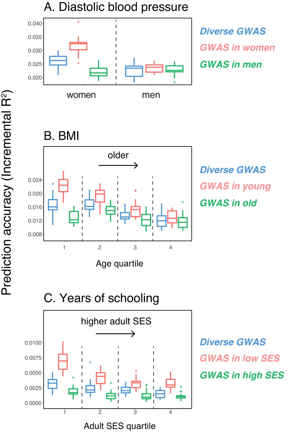
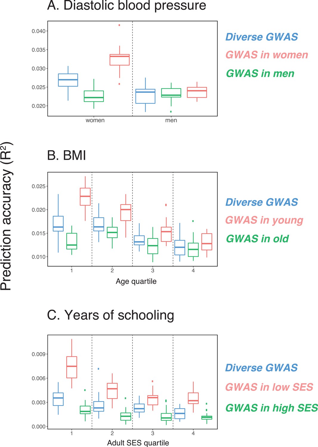
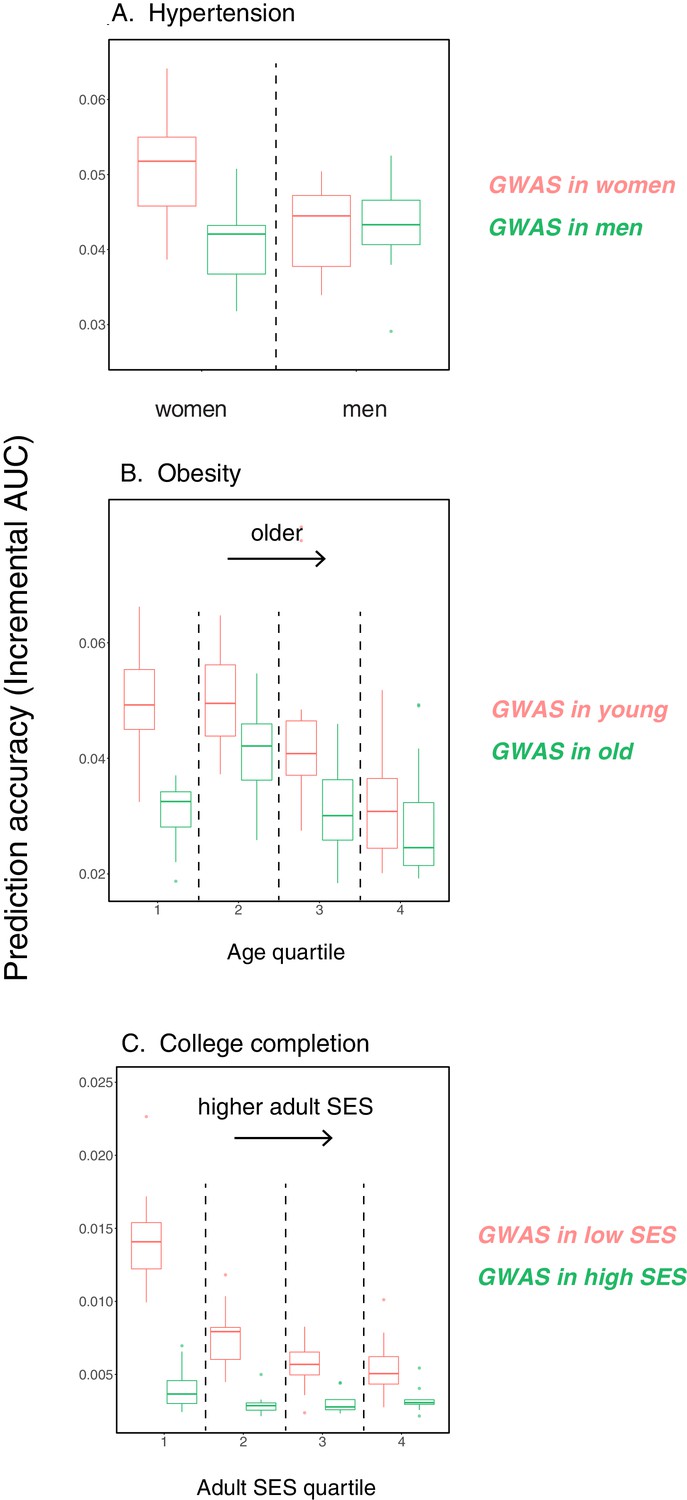
Variable prediction accuracy of polygenic scores within an ancestry group.
Shown are incremental values (i.e., the increment in obtained by adding a polygenic score predictor to a model with covariates alone) in different prediction sets. Each box and whiskers plot is computed based on 20 iterations of resampling GWAS and prediction sets. Thick horizontal lines denote the medians. The polygenic scores were estimated in samples of unrelated WB individuals. Phenotypes were then predicted in distinct samples of unrelated WB individuals, stratified by sex (A), age (B) or Townsend deprivation index, a measure of SES (C). In red and green cases, polygenic scores are based on a GWAS in a sample limited to one sex, age or SES group (a 'stratum'). In blue, polygenic scores are based on a GWAS in a diverse sample matching the number of individuals in each stratum. GWAS samples sizes are: 122,774 for all three diastolic blood pressure GWAS samples, 72,328 for all three BMI GWAS samples, 73,280 for years of schooling GWAS in the diverse sample and 73,283 for GWAS in the low SES and high SES samples.
Figure 2
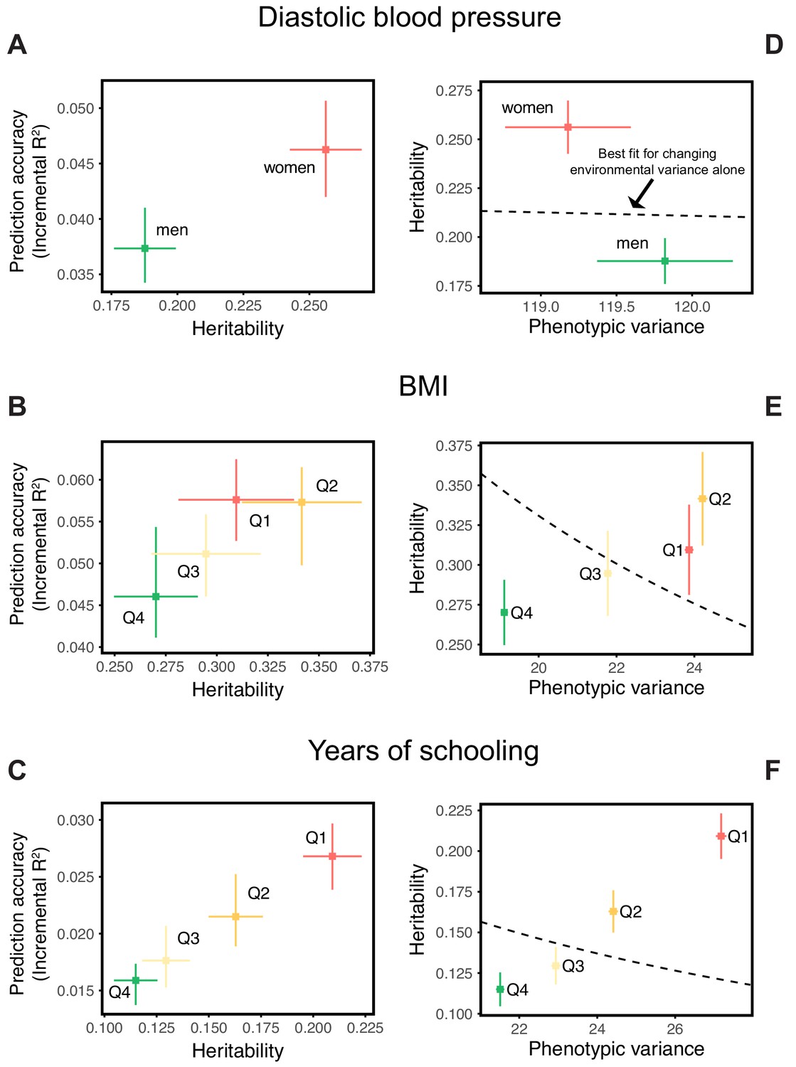
Differences in environmental variance alone do not explain the variable prediction accuracy.
(A,B,C) The x-axes show heritability estimates (± SE) based on LD score regression in each set. The y-axes show incremental values obtained using the procedure described in Figure 1, with GWAS performed in a pooled sample of all strata and testing in stratified prediction sets (see Materials and methods); points and bars show mean and central 80% range computed based on 20 iterations of resampling GWAS and prediction sets. ‘Q’ denotes quartile of age and SES in (B,E) and (C,F), respectively. (D,E,F) The x-axes show phenotypic variance estimates (± SE) across strata after adjusting for covariates (sex, age and 20 PCs). If the heritability differences across strata are due to differences in environmental variance alone, with genetic variance constant, then heritability should be inversely proportional to phenotypic variance. The best-fitting model for this inverse proportionality (dashed line, simple linear regression) provides a poor fit to the observations.
Figure 3
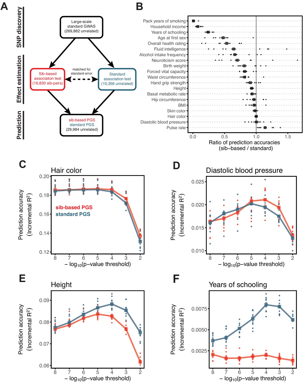
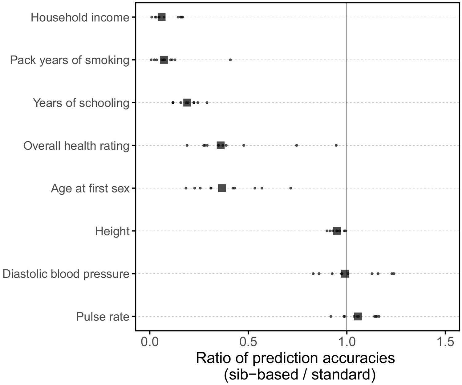
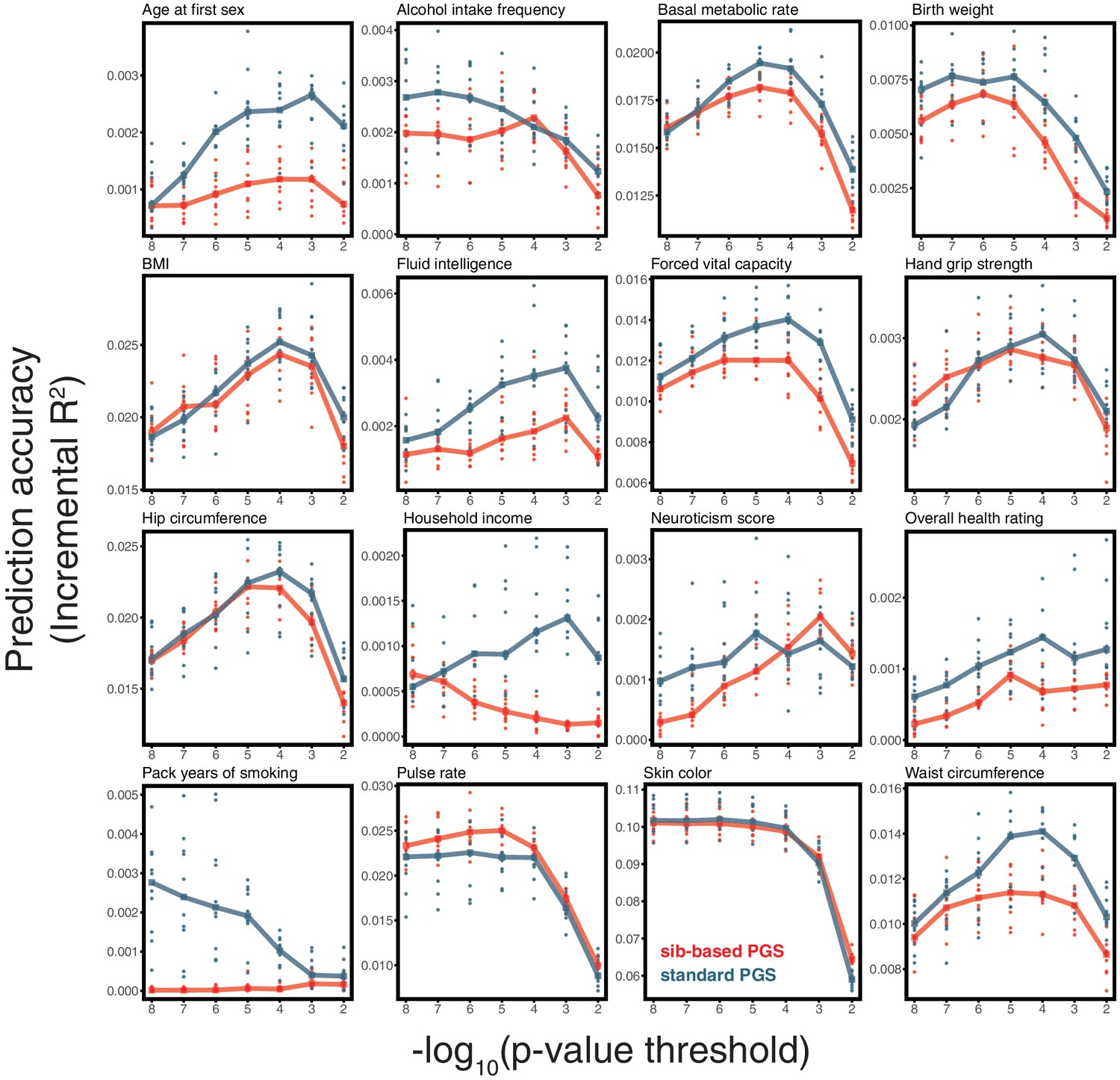
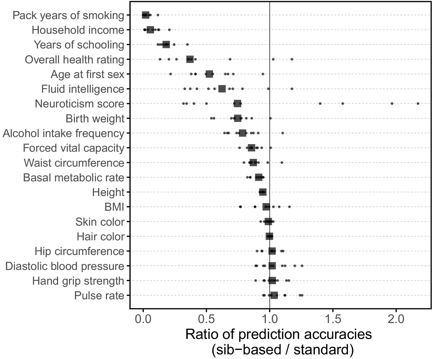
Comparison of prediction accuracy of standard and sib-based polygenic scores.
(A) After ascertaining SNPs in a large sample of unrelated individuals, we estimated the effects of these SNPs with a standard regression using unrelated individuals and, independently, using sib-regression. We then used the polygenic scores for prediction in a third sample of unrelated individuals. We chose the sample size of the standard PGS estimation set such that median effect estimate SEs are equal in the two designs, thereby ensuring equal prediction accuracy under a vanilla model with no indirect effects or assortative mating. Numbers in parentheses are median sample size in each set across 20 traits (see Materials and methods and Appendix 1—table 1 for the definition of each trait, and Appendix 1—table 3 for sample sizes for each trait). (B) Ratio of prediction accuracy in the two designs across 20 traits. For each trait, we performed 10 resampling iterations of unrelated individuals into three sets for discovery, estimation and prediction (small points). Large points show median values. (C-F) We repeated this procedure with different discovery-set p-value thresholds for including a SNP in the polygenic score. The higher the p-value threshold is, the more SNPs are included. For each p-value threshold, points show 10 iterations as described and large points show median values. Shown are a subset of traits, with traits appearing in (B) but not shown here presented in Appendix 1—figure 12.
Appendix 1—figure 1
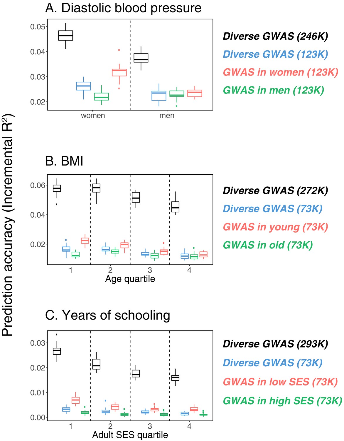
Variable prediction accuracy within an ancestry group.
This figure extends Figure 1 of the main text, showing prediction accuracies based on large-scale diverse GWAS that are the union of all strata matching the number of individuals in each stratum. The numbers in parentheses show GWAS sample sizes (see Materials and methods for details). Each box and whiskers plot was computed based on 20 iterations of resampling estimation and prediction sets. Thick horizontal lines denote the medians. The polygenic scores were estimated in samples of unrelated WB individuals. Phenotypes were then predicted in distinct samples of unrelated WB individuals, stratified by sex (A), age (B) or Townsend deprivation index, a measure of SES (C). In red and green cases, polygenic scores are based on a GWAS in a sample limited to one sex, age or SES group (a 'stratum’). In black, polygenic scores are based on a diverse GWAS in a pooled sample of all strata. In blue, polygenic scores are based on a diverse GWAS in a pooled sample of all strata but downsampled to match the size of the stratified GWAS.
Appendix 1—figure 2
Variable prediction accuracy (measured as ) within an ancestry group.
This figure mirrors Figure 1 of the main text, except for the y-axis showing values (squared correlation between polygenic score and phenotype residualized on covariates), rather than incremental . Each box and whiskers plot was computed based on 20 iterations of resampling estimation and prediction sets. Thick horizontal lines denote the medians. The polygenic scores were estimated in samples of unrelated WB individuals. Phenotypes were then predicted in distinct samples of unrelated WB individuals, stratified by sex (A), age (B) or Townsend deprivation index, a measure of SES (C). In red and green cases, polygenic scores are based on a GWAS in a sample limited to one sex, age or SES group (a 'stratum’). In blue, polygenic scores are based on a GWAS in a diverse sample of all strata downsampled to match the size of the stratified GWAS.
Appendix 1—figure 3
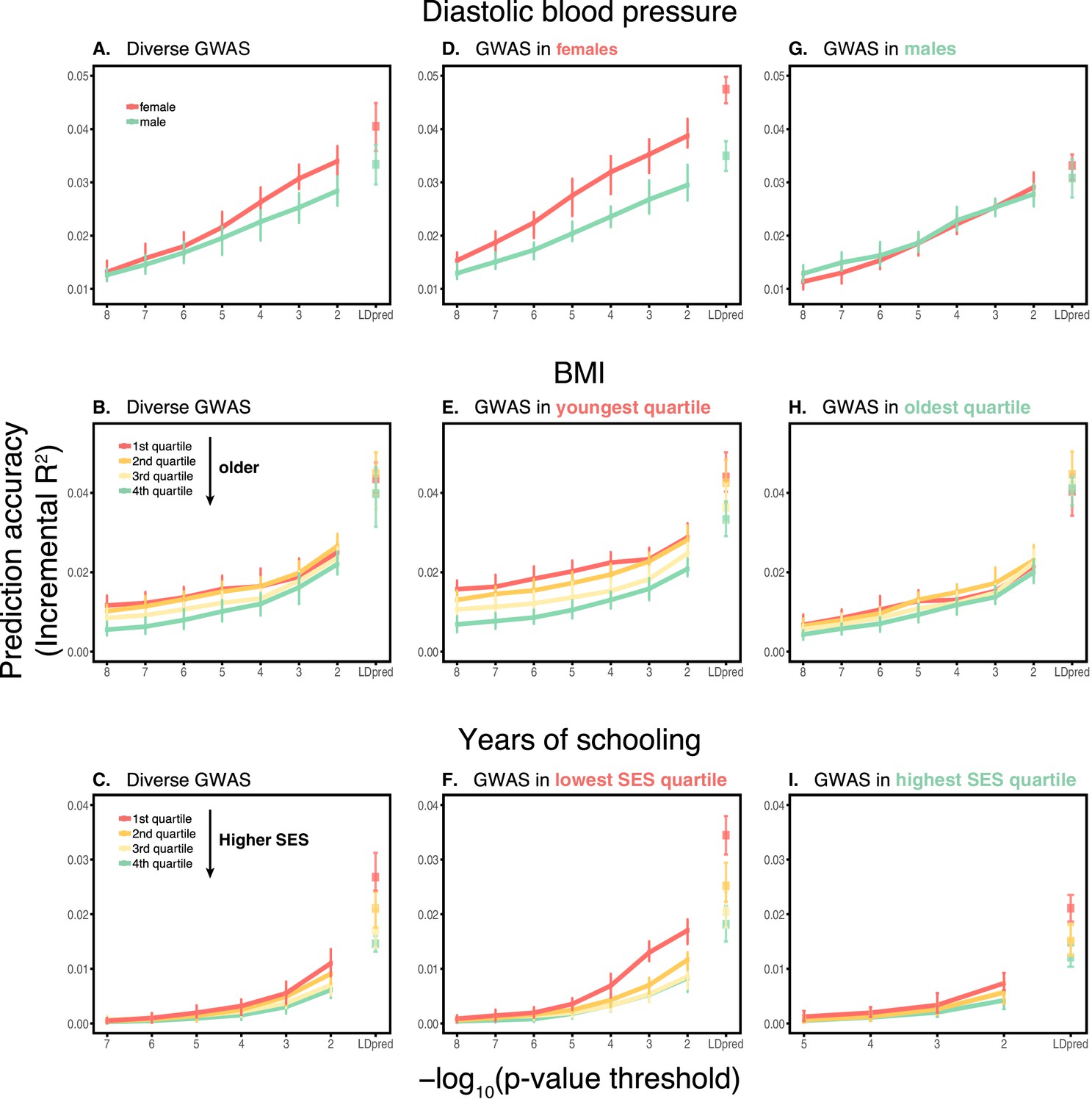
Dependence on the polygenic score model.
This figure extends Figure 1 of the main text, showing the prediction accuracies as a function of the p-value threshold for inclusion of a SNP in the polygenic score when based on a pruning and thresholding approach. The higher the p-value threshold is, the more SNPs are included. Last points on the x-axis correspond to a polygenic score model based on the LDpred approach (Vilhjálmsson et al., 2015) with a prior probability of 1 on loci being causal. Shown are incremental values in different prediction sets. Points and error bars are mean and central 80% range computed based on 20 iterations of resampling estimation and prediction sets. (A–C) The polygenic scores were estimated in samples of unrelated WB individuals. Phenotypes were then predicted in distinct samples of unrelated WB individuals, stratified by sex (A), age (B) or Townsend deprivation index, a measure of SES (C). (D–I) Same as in A-C, but here the polygenic scores are based on a GWAS in a sample limited to one sex, age or SES group. The trends shown in Figure 1 of the main text are for p-value threshold of 10−4, and are qualitatively similar to the trends for other choices of the polygenic score model. For each trait, sample sizes are matched across all GWAS sets.
Appendix 1—figure 4
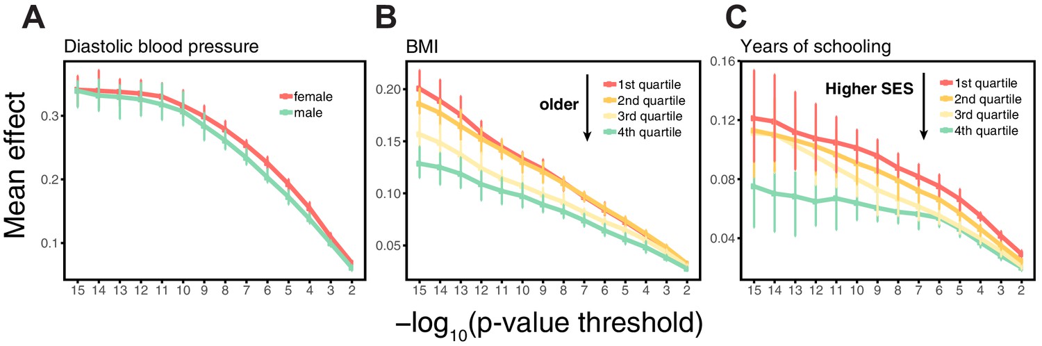
Estimating mean effect size across strata.
SNPs were ascertained in large samples of unrelated WB individuals. The effects of trait-increasing alleles were then re-estimated in an independent set of unrelated WB individuals (that were excluded from the original GWAS) stratified by sex for diastolic blood pressure (A), by age for BMI (B) and by Townsend deprivation index, a measure of SES for years of schooling (C). Points and error bars are mean and central 80% range computed based on 20 iterations of resampling ascertainment and estimation sets, plotted as a function of the p-value threshold (for p-values obtained in the discovery GWAS).
Appendix 1—figure 5
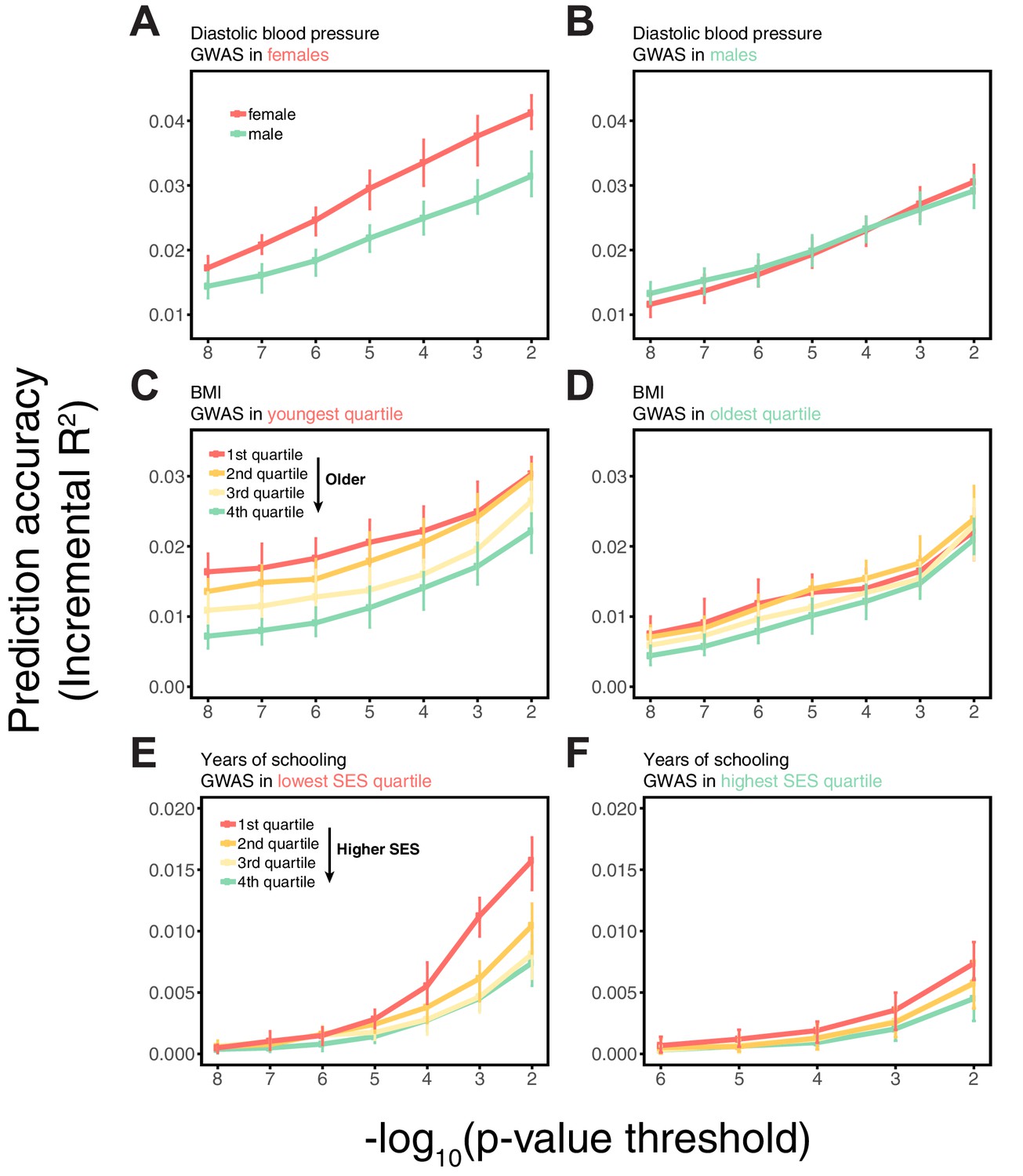
Variable prediction accuracy within an ancestry also seen using a linear mixed model.
This figure mirrors the last two columns in Appendix 1—figure 3, except that here, the GWAS estimates were obtained from a linear mixed model (LMM) (Loh et al., 2015). Shown are the prediction accuracies, measured as incremental , as a function of the p-value threshold for inclusion of a SNP in the polygenic score. Points and error bars are mean and central 80% range computed based on 20 iterations of resampling estimation and prediction sets. The polygenic scores are based on a GWAS in a sample limited to one sex, age or SES group. Phenotypes are then predicted in distinct samples of unrelated individuals, stratified by sex (A,B), age (C,D) or Townsend deprivation index, as a measure of SES (E,F). The qualitative trends are similar to those in Appendix 1—figure 3, which uses a standard linear regression with PCs (principal components of the genotype data) as a control for population structure when testing for an association between the phenotypes and genotypes. The similarity suggests that the observed differences in prediction accuracies across strata are not driven to a large degree by population structure confounding.
Appendix 1—figure 6
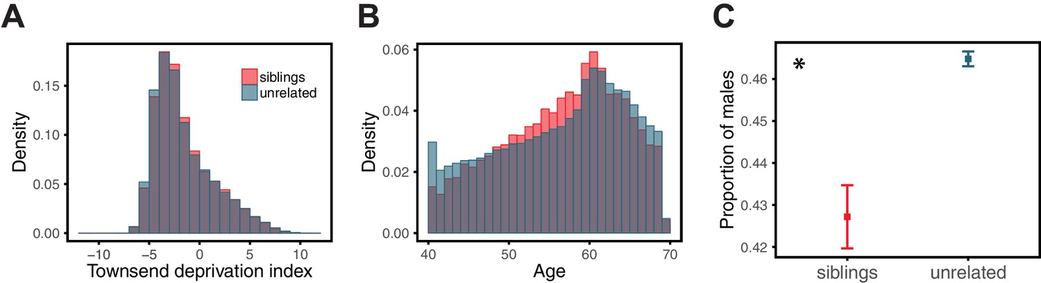
Comparison of siblings and unrelated individuals in the UK Biobank with respect to age, SES, and sex ratio.
Panels show the distribution of Townsend deprivation index, a measure of SES (A), the age distribution (B), and the proportion of males (C) for the siblings and unrelated sets used in the analysis described for Figure 3 of the main text. For each sibling pair, one sibling was randomly selected for these comparisons. The asterisk symbol marks a significant difference at the 1% level between siblings and unrelated individuals, as assessed by a Mann-Whitney test. SES and age distributions are quite similar in siblings and unrelated sets, whereas the proportion of males is significantly smaller in the siblings.
Appendix 1—figure 7

Comparison of siblings and unrelated individuals in the UK Biobank with respect to population structure.
Panels show the distribution of PCs (principal components of the genotype data) for the siblings and unrelated sets used in the analysis described for Figure 3 of the main text. For each sibling pair, one sibling was randomly selected for these comparisons. The asterisk symbol marks a significant difference at the 1% level between siblings and unrelated individuals, as assessed by a Mann-Whitney test. Despite slight but significant differences, siblings and unrelated sets are broadly similar with respect to their genetic ancestries.
Appendix 1—figure 8
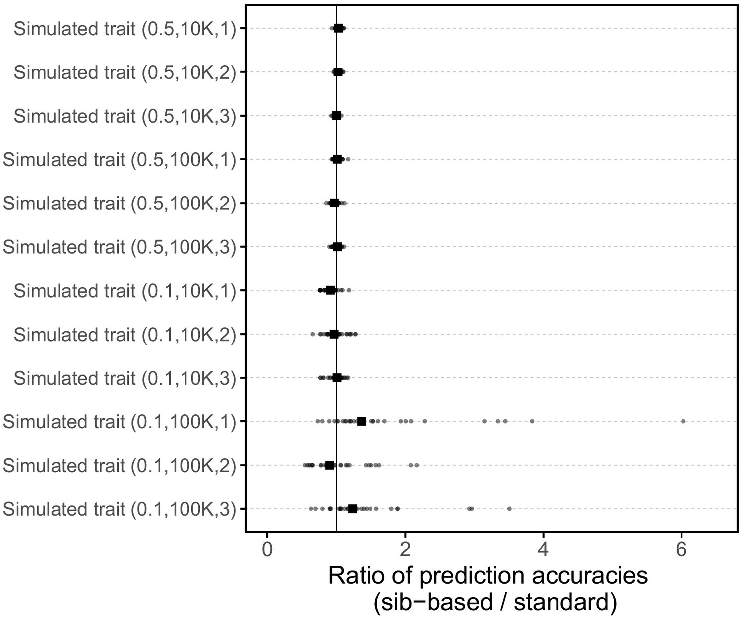
Comparison of prediction accuracies of polygenic scores based on standard and sib-GWAS for simulated traits.
This figure mirrors Figure 3B of the main text, but here plotted for 12 simulated traits. The numbers in parentheses are the heritability, the number of causal loci considered, and the simulation replicate number, respectively. Three traits were simulated for each pair of heritability and number of causal loci parameters (see Materials and methods for simulation details). Small points show the ratio of the prediction accuracies in the two designs across 30 iterations; in each iteration, we resample sets of unrelated individuals to constitute three sets for discovery, estimation and prediction. Larger points show median values.
Appendix 1—figure 9
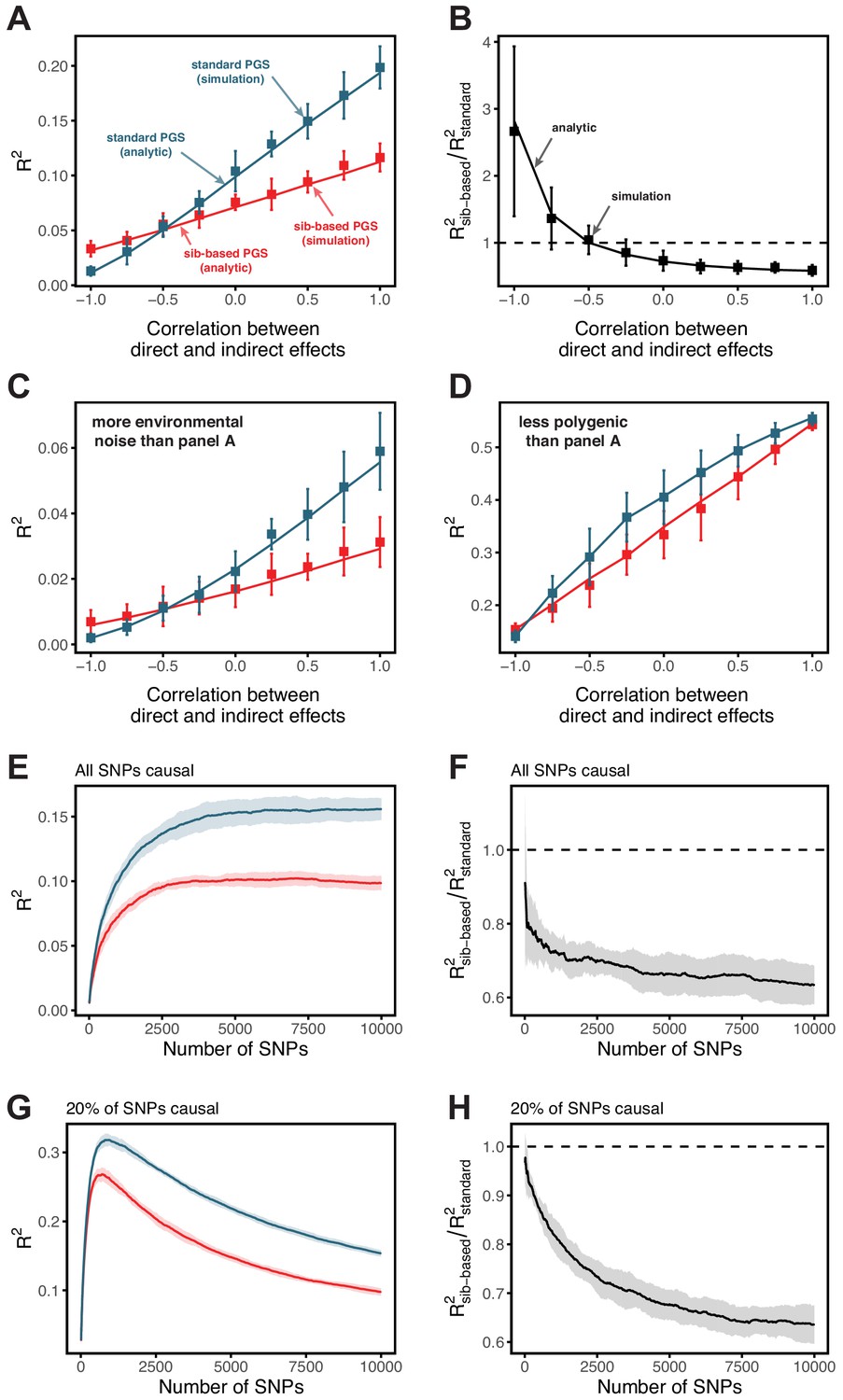
Simulation results for polygenic scores based on standard GWAS and sib-GWAS in the presence of indirect effects.
(A,B) Simulation results as a function of the correlation between direct and indirect effects, . Simulations were performed with , , and . The size of the estimation set in the sib-GWAS is 10,000, and the size of the estimation set in the standard GWAS is chosen to match sampling variances between the two study designs. The polygenic scores is based on 10,000 causal loci; its performance was evaluated in an independent set of 10,000 unrelated individuals. As long as direct and indirect effects are not strongly negatively correlated, the out of sample prediction accuracy is higher for the polygenic scores based on standard GWAS. (C) Same as (A) but with three-fold greater environmental noise. (D) Same as (A) but with 100 causal loci. In (A–D) points are mean ± 2 SD in 10 simulation iterations. Solid lines are values based on analytic expressions derived in Section 1.3.2. (E–H) Simulation results, with the same parameters as in (A) but , as a function of the number of SNPs included in the polygenic scores, with all loci being causal (E,F), or with 20% of loci being causal (G,H). SNPs are added in increasing order of their association p-value in an independent set of 20,000 unrelated individuals. In both cases, the ratio of prediction accuracies of polygenic scores based on sib- versus standard GWAS becomes smaller with the inclusion of more weakly associated SNPs, a behavior qualitatively similar to observations in Figure 3 in the main text. Points are mean ± 2 SD in 10 simulations. See Section 1.3.3 for simulation details.
Appendix 1—figure 10
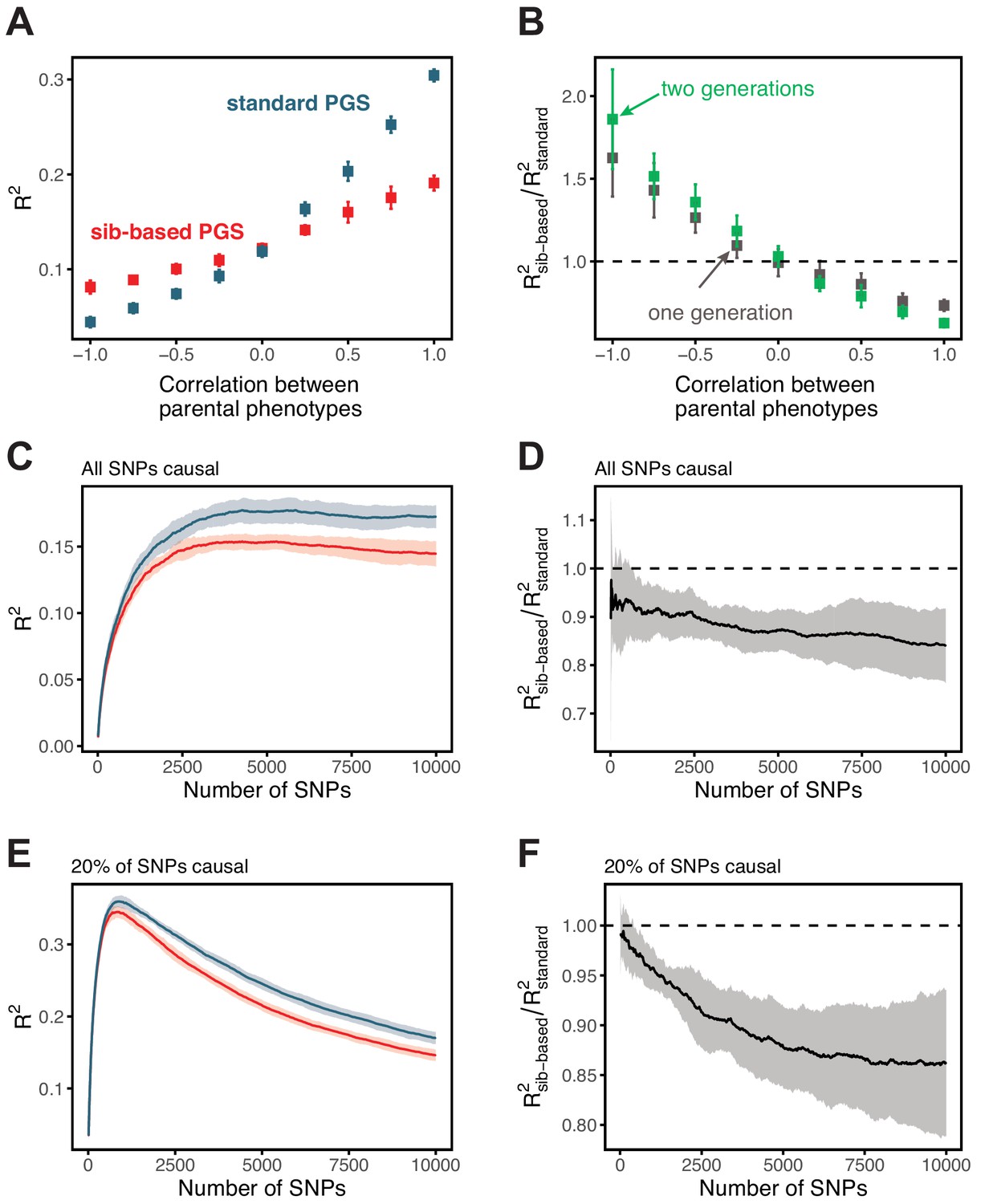
Simulation results for polygenic scores based on standard GWAS and sib-GWAS in the presence of assortative mating.
(A) Simulation results as a function of the approximate correlation between parental phenotypes, . Simulations were performed with under random mating. The size of the estimation set in the sib-GWAS is 10,000, and the size of the estimation set in the standard GWAS is chosen to match sampling variances between the two study designs. The polygenic score is based on 10,000 causal loci; its performance was evaluated in an independent set of 10,000 unrelated individuals. Standard-GWAS based polygenic scores outperforms (underperforms) sib-GWAS based polygenic scores under positive (negative) assortative mating. (B) Ratio of prediction accuracies of the polygenic scores based on sib- versus standard GWAS, as a function of , for two sets of simulations with one or two generations of assortative mating, with same parameters as in (A). (C–F) Simulation results, with the same parameters as in (A) but , as a function of the number of SNPs included in the polygenic score, with all loci being causal (C,D), or with 20% of loci being causal (E,F). SNPs are added in the order of their association p-value in an independent set of 20,000 unrelated individuals. In both cases, the ratio of prediction accuracies for scores based on sib-GWAS versus standard GWAS becomes smaller with the inclusion of more weakly associated SNPs, a behavior that is qualitatively similar to observations in Figure 3 in the main text. Points are mean ± 2 SD in 10 simulation iterations. See Section 1.4.1 for simulation details.
Appendix 1—figure 11
Comparison of prediction accuracies of polygenic scores based on standard and sib-GWAS matched for sex ratio.
This figure mirrors Figure 3B of the main text, but here the samples of siblings and unrelated individuals used in the analysis are matched for their sex ratios. Results are shown for diastolic blood pressure, as the prediction accuracy differed between sexes (Figure 1); the related phenotype of pulse rate; and a subset of the traits for which the prediction accuracy varied by GWAS design (Figure 3B). Small points show the ratio of the prediction accuracies in the two designs across 10 iterations; in each iteration, we resample sets of unrelated individuals to constitute three sets for discovery, estimation and prediction. Larger points show median values. We note that pulse rate is now similarly predicted by the two GWAS approaches, suggesting that perhaps the slightly higher prediction accuracy of the sib-GWAS shown in the main text Figure 3B are due to the sex ratio difference; for other traits, results are qualitatively unchanged.
Appendix 1—figure 12
Prediction accuracy of polygenic scores based on sib-and standard GWAS, for a range of traits.
This figure complements Figure 3C–F of the main text, showing the results of the study design depicted in Figure 3A for all traits presented in Figure 3. As described for Figure 3, we randomly divided unrelated individuals to constitute three non-overlapping sets for discovery, estimation and prediction. Small points correspond to 10 iterations of resmapling these three sets. The prediction accuracy is plotted as a function of the p-value threshold, where p-values come from the discovery GWAS. Lines show median values.
Appendix 1—figure 13
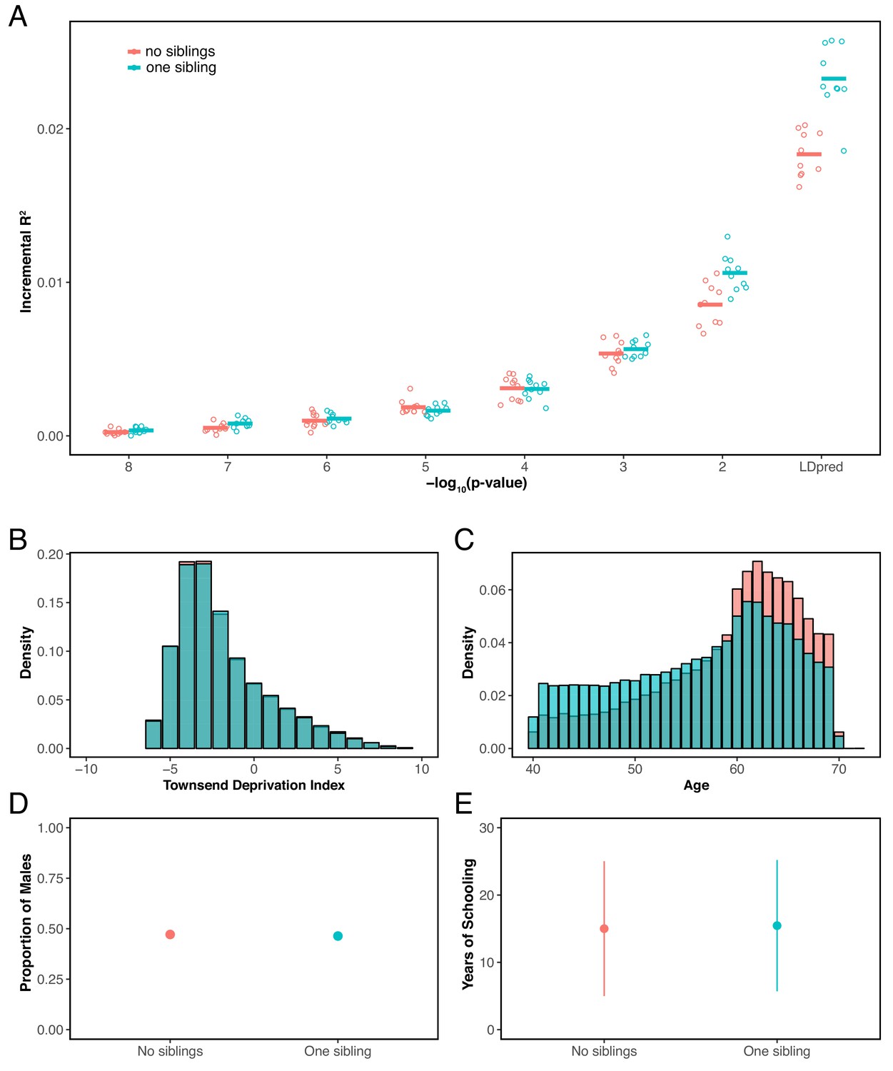
Prediction accuracy for years of schooling, for individuals with 0 or 1 full sibling.
(A) The y-axis shows the prediction accuracy, measured as incremental , in prediction sets stratified by participants’ number of siblings, using a polygenic score for years of schooling based on a GWAS performed using individuals who reported to have exactly 1 sibling. The x-axis shows the p-value threshold for inclusion of a SNP in the polygenic score when based on a pruning and thresholding approach. Last points on the x-axis correspond to a polygenic score model based on the LDpred approach (Vilhjálmsson et al., 2015) with a prior probability of 1 on loci being causal. Points are values based on 10 iterations of resampling estimation and prediction sets. Thick horizontal lines denote the mean values. (B–E) Comparison of the distribution of Townsend deprivation index (B) the age distribution (C), the proportion of males (D), and mean years of schooling (± 2 SD) between individuals who reported having no sibling and those who reported having 1 sibling. The two sets have somewhat different distributions of ages (or possibly come from somewhat different birth cohorts), a feature that could contribute to the patterns seen in panel A, but are otherwise similar with respect to the other features considered.
Appendix 1—figure 14
Variable prediction accuracy for binary traits, when measured as incremental AUC.
This figure is analogous to the one shown in Figure 1 of the main text, but considering dichotomized versions of the traits presented in Figure 1 in the prediction sets, and with the y-axis showing incremental AUC values rather than incremental . The polygenic scores are based on GWAS using the quantitative trait values as in Figure 1. The traits are (A) diastolic blood pressure of over 110 mmHg, (B) BMI of over 35 Kg/m2, and (C) completing a college or a university degree. Each box and whiskers plot was computed based on 20 iterations of resampling estimation and prediction sets. Thick horizontal lines denote the medians.
Appendix 1—figure 15
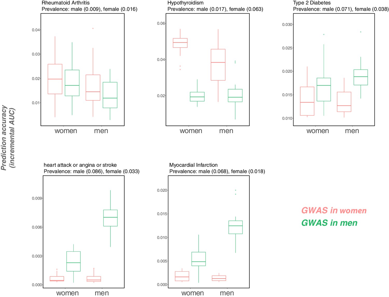
Variable prediction accuracy for binary disease phenotypes, measured as incremental AUC, in men versus women.
This figure is analogous to the one shown in Figure 1 of the main text, but looking at disease traits, and with the y-axis showing incremental AUC rather than incremental . Each box and whiskers plot was computed based on 20 iterations of resampling estimation and prediction sets. Thick horizontal lines denote the medians. The variable prediction accuracy of PGS based on GWAS in men only versus women only could be driven in part by the differences in ratios of cases to controls (and hence by differences in the precision of the effect size estimates). However, we also observe that the prediction accuracy can vary depending on the sex composition of the prediction set (e.g., for cardiovascular outcomes), an observation that cannot be attributed to differences in case:control ratios of the GWAS.
Appendix 1—figure 16
Comparison of prediction accuracies of polygenic scores (measured as ) based on standard and sib-GWAS.
This figure mirrors Figure 3B of the main text, but here we first residualized the phenotypes on covariates, and then ran the same pipeline described as that used to generate Figure 3B on the residuals without further adjustment for covariates in the GWAS or prediction evaluation. Thus, this figure relates more directly to the analytical derivation in Section 1.2. However, the results in Figure 3B and here are qualitatively similar. Small points show the ratio of the prediction accuracies in the two designs across 10 iterations; in each iteration, we resample sets of unrelated individuals to constitute three sets for discovery, estimation and prediction. Larger points show median values.
Tables
Appendix 1—table 1
UK Biobank phenotype data used in this study and their corresponding data fields.
In parentheses are the units of measurements.
| Trait | Description | UKB data field |
|---|---|---|
| Age | Age when attended assessment center (years) | 21003 |
| Age at first sex | Self-reported age at first sexual intercourse (years) | 2139 |
| Alcohol intake frequency | Self-reported category, encoded as an integer: 1, 'Daily or almost daily’; 2, 'Three or four times a week’; 3, 'Once or twice a week’; 4, 'One to three times a month’; 5, 'Special occasions only’; 6, 'Never’ | 1558 |
| Basal metabolic rate | Estimated from body composition impedance measurements (KJ) | 23105 |
| Birth weight | Self-reported birth weight (Kg) | 20022 |
| Body mass index | Constructed from height and weight measurements (Kg/m2) | 21001 |
| Diastolic blood pressure | Measured using automated devices (mmHg); values are adjusted for medicine use (see Materials and methods) | 4079, 6153, 6177 |
| Fluid intelligence | Unweighted sum of the number of correct answers given to 13 fluid intelligence questions | 20016 |
| Forced vital capacity | Calculated from breath spirometry (liters) | 3062 |
| Hair color | Self-reported category, encoded as an integer: 1, 'Blonde’; 2, 'Red’; 3, 'Light brown’; 4, 'Dark brown’; 5, 'Black’; none, 'Other’ | 1747 |
| Hand grip strength | Measured right and left hand isometric grip strength (Kg) | 46, 47 |
| Height | Measured standing height (cm) | 50 |
| Hip circumference | Measured hip circumference (cm) | 49 |
| Hospital inpatient diagnoses | Diagnoses made during hospital inpatient admissions, coded according to the International Classification of Diseases (ICD-9 and ICD-10) | 41202, 41203, 41204, 41205, 41270, 41271 |
| Household income | Self-reported average total annual household income before tax category, encoded as an integer: 1, 'Less than £18,000'; 2, '£18,000 to £30,999'; 3, '£31,000 to £51,999'; 4, '£52,000 to £100,000'; 5, 'Greater than £100,000' | 738 |
| Myocardial infarction outcomes | Algorithmically-defined myocardial infarction outcomes obtained through combinations of UK Biobank's assessment data collection (e.g., self-reported conditions), and data from hospital admissions | 42000, 42001 |
| Neuroticism score | Derived summary score, based on participants’ responses to 12 neurotic behaviour-related questions | 20127 |
| Number of full siblings | Sum of self-reported number of full brothers and full sisters | 1873, 1883 |
| Overall health rating | Self-reported category, encoded as an integer: 1, 'Excellent'; 2, 'Good'; 3, 'Fair'; 4, 'Poor’ | 2178 |
| Pack years of smoking | Calculated for individuals who have ever smoked as the number of cigarettes smoked per day, divided by twenty, multiplied by the number of years of smoking (years) | 20161 |
| Pulse rate | Measured during the automated blood pressure readings (bpm) | 102 |
| Qualifications | Self-reported educational or professional qualifications, selected from: 'College or University degree', 'NVQ or HND or HNC or equivalent', 'Other professional qualifications eg: nursing, teaching', 'A levels/AS levels or equivalent', 'O levels/GCSEs or equivalent', 'CSEs or equivalent', or 'None of the above' | 6138 |
| Sex | Self-reported sex and as determined from genotyping analysis | 31, 22001 |
| Skin color | Self-reported category, encoded as an integer: 1, 'Very fair'; 2, 'Fair'; 3, 'Light olive'; 4, 'Dark olive'; 5, 'Brown'; 6, 'Black' | 1717 |
| Townsend deprivation index | Townsend deprivation index at recruitment | 189 |
| Vascular/heart problems | Self-reported vascular/heart problems diagnosed by doctor selected from the categories: 'Heart attack’, 'Angina', 'Stroke', 'High blood pressure', and 'None of the above' | 6150 |
| Waist circumference | Measured waist circumference (cm) | 48 |
Appendix 1—table 2
Genetic correlations across samples that vary by a study characteristic.
Numbers are genetic correlations estimated using LD score regression for BMI, years of schooling and diastolic blood pressure, across samples stratified by age, Townsend deprivation index (a measure of socioeconomic status, SES), and sex, respectively. ’Q’ denotes quartile of age or SES.
| Trait/characteristic | Pair of strata | Genetic correlation (s.e.) |
|---|---|---|
| BMI/Age | (Q1,Q2) | 0.93 (0.036) |
| (Q1,Q3) | 0.95 (0.035) | |
| (Q1,Q4) | 0.95 (0.038) | |
| (Q2,Q3) | 0.89 (0.032) | |
| (Q2,Q4) | 0.91 (0.036) | |
| (Q3,Q4) | 1.00 (0.040) | |
| Years of schooling/SES | (Q1,Q2) | 0.98 (0.054) |
| (Q1,Q3) | 1.00 (0.067) | |
| (Q1,Q4) | 0.93 (0.068) | |
| (Q2,Q3) | 0.97 (0.064) | |
| (Q2,Q4) | 1.09 (0.074) | |
| (Q3,Q4) | 1.04 (0.074) | |
| Diastolic blood pressure/Sex | (male,female) | 0.93 (0.031) |
Appendix 1—table 3
Sample sizes used for siblings and unrelated sets.
As described in Figure 3A, for the comparison of prediction accuracies of polygenic scores based on standard and sib-GWAS, we first ascertain SNPs in a large sample of unrelated individuals (‘Unrelated-discovery’) and then estimate the effect of these SNPs with a standard regression using unrelated individuals (‘Unrelated-n*') and, independently, using sib-regression (in the ‘Siblings’ set). Finally, we used the polygenic scores for prediction in a third sample of unrelated individuals (‘Unrelated-prediction’). This table shows sample sizes used for each set across the traits analyzed. For simulated traits, the numbers in parentheses are heritability, number of causal loci, and simulation replicate, respectively (three traits were simulated for each pair of heritability and number of causal loci parameters, see Materials and methods for simulation details).
| Trait | Siblings (pairs) | Unrelated-n* | Unrelated- discovery | Unrelated- prediction |
|---|---|---|---|---|
| Age at first sex | 13675 | 8746 | 244988 | 27220 |
| Alcohol intake frequency | 17282 | 10923 | 276885 | 30764 |
| Basal metabolic rate | 16802 | 13467 | 269750 | 29972 |
| Birth weight | 6750 | 5766 | 159074 | 17674 |
| BMI | 17217 | 12359 | 274868 | 30540 |
| Diastolic blood pressure | 14791 | 9514 | 253227 | 28136 |
| Fluid intelligence | 3889 | 2979 | 101016 | 11223 |
| Forced vital capacity | 14605 | 10009 | 252576 | 28064 |
| Hair color | 16859 | 11763 | 272209 | 30245 |
| Hand grip strength | 17070 | 10832 | 275117 | 30568 |
| Height | 17242 | 18147 | 269973 | 29997 |
| Hip circumference | 17254 | 11648 | 275930 | 30658 |
| Household income | 13240 | 8704 | 239326 | 26591 |
| Neuroticism score | 11756 | 6909 | 227010 | 25223 |
| Overall health rating | 17189 | 10378 | 276581 | 30731 |
| Pack years of smoking | 2307 | 1682 | 85544 | 9504 |
| Pulse rate | 14791 | 8812 | 253859 | 28206 |
| Skin color | 16903 | 10334 | 274159 | 30462 |
| Waist circumference | 17257 | 11749 | 275873 | 30652 |
| Years of schooling | 17037 | 11885 | 273553 | 30394 |
| Simulated trait (0.5,10K,1) | 17299 | 11685 | 276404 | 30711 |
| Simulated trait (0.5,10K,2) | 17299 | 11505 | 276566 | 30729 |
| Simulated trait (0.5,10K,3) | 17299 | 11422 | 276641 | 30737 |
| Simulated trait (0.5,100K,1) | 17299 | 11814 | 276288 | 30698 |
| Simulated trait (0.5,100K,2) | 17299 | 11833 | 276271 | 30696 |
| Simulated trait (0.5,100K,3) | 17299 | 11490 | 276579 | 30731 |
| Simulated trait (0.1,10K,1) | 17299 | 9072 | 278756 | 30972 |
| Simulated trait (0.1,10K,2) | 17299 | 9158 | 278678 | 30964 |
| Simulated trait (0.1,10K,3) | 17299 | 9111 | 278721 | 30968 |
| Simulated trait (0.1,100K,1) | 17299 | 9133 | 278701 | 30966 |
| Simulated trait (0.1,100K,2) | 17299 | 9069 | 278758 | 30973 |
| Simulated trait (0.1,100K,3) | 17299 | 9108 | 278723 | 30969 |
Appendix 1—table 4
Qualifications to years of schooling conversion table.
Educational or professional qualifications were converted to years of schooling following Okbay et al. (2016).
| Qualifications (UKB data field 6138) | Years of schooling |
|---|---|
| College or University degree | 20 |
| NVQ or HND or HNC or equivalent | 19 |
| Other professional qualifications eg: nursing, teaching | 15 |
| A levels/AS levels or equivalent | 13 |
| O levels/GCSEs or equivalent | 10 |
| CSEs or equivalent | 10 |
| None of the above | 7 |
Additional files
Download links
A two-part list of links to download the article, or parts of the article, in various formats.
Downloads (link to download the article as PDF)
Open citations (links to open the citations from this article in various online reference manager services)
Cite this article (links to download the citations from this article in formats compatible with various reference manager tools)
Variable prediction accuracy of polygenic scores within an ancestry group
eLife 9:e48376.
https://doi.org/10.7554/eLife.48376


