Figures and data in Velocity coupling of grid cell modules enables stable embedding of a low dimensional variable in a high dimensional neural attractor | eLife

Figures
Additional files

7 figures and 1 additional file

Figures

Figure 1

Download asset Open asset

Velocity coupling: illu.

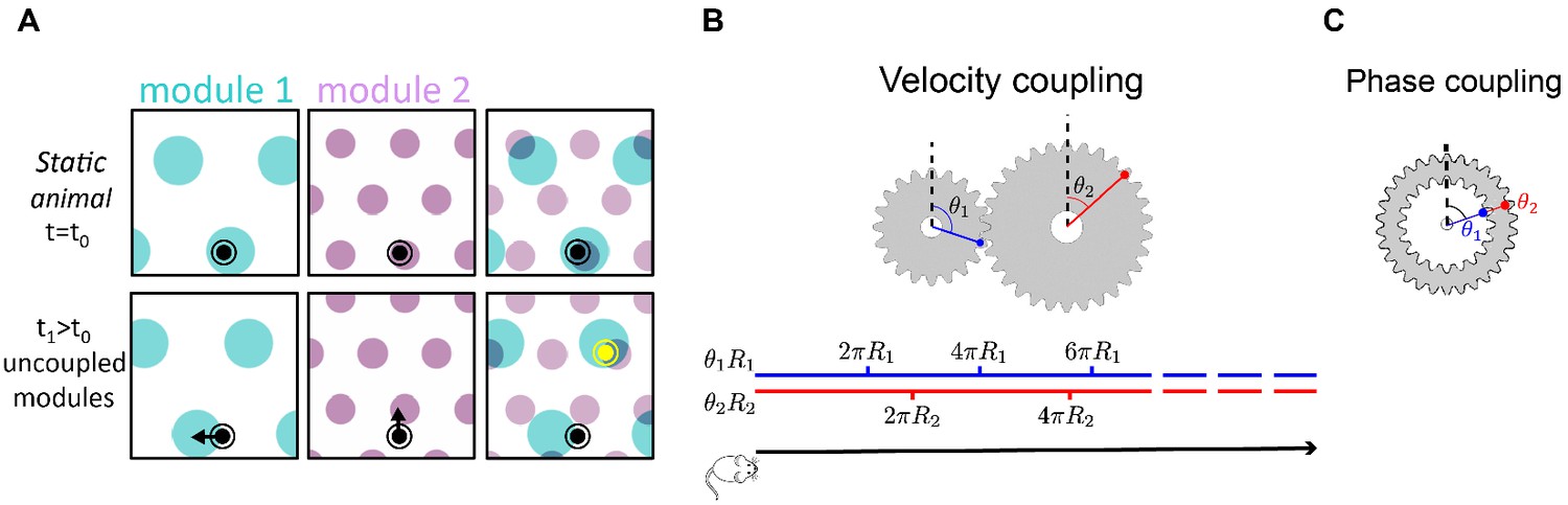
(A) Illustration of the detrimental consequences arising from uncoupled module drifts. Black dot: location of a static animal. Top panels: schematic representation of the decoded position from the neural activity in module 1 (left panel) and module 2 (middle panel) at time $t = t_{0}$ . The shaded areas (cyan, purple) represent locations whose likelihood, given the neural activity, is high. Top right panel: overlay of the likelihood read out from module 1 and module 2. The maximal likelihood location, based on activity in both modules, coincides with the animal’s position. Bottom panels: decoded position based on the neural activity at time $t_{1}$ . Due to independent, noise-driven drifts in each module, activity in module 1 represents positions that are slightly shifted to the left (bottom left), and activity in module 2 represents position that are slightly shifted upward (middle). Even though the shifts are small, the joint activity in both modules (bottom right) now represents a new maximum likelihood location (yellow), far away from the true location (black). We refer to such events as catastrophic readout errors. (B) Representation of position along a one-dimensional axis (black line) by the rotation angles $θ_{1}$ and $θ_{2}$ of two meshing gears that rotate in a coordinated manner in response to motion. The angles $θ_{1}$ and $θ_{2}$ , corresponding to each position, are shown along the blue and red lines. If the radii $R_{1}$ and $R_{2}$ are incommensurate, a large range of positions can be unambiguously read out from the combination of the two angles. (C) An example of two phase coupled meshing gears that are fixed to each other, such that their angles $θ_{1}$ and $θ_{2}$ are always identical. Since $θ_{1} = θ_{2}$ , there is effectively only one encoded angle, and the range of unambiguous representation corresponds to a single rotation of the gears.

https://doi.org/10.7554/eLife.48494.002

Figure 2

Download asset Open asset

Model architecture.

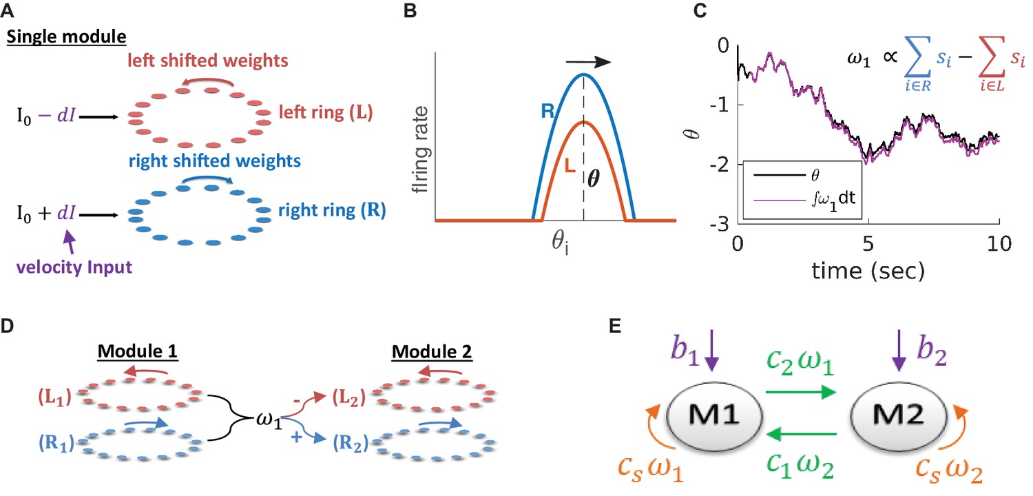
(A) Structure of a single module, consisting of a left ring (red) and a right ring (blue), in accordance with the double ring model (Xie et al., 2002). The two rings receive external inputs proportional to velocity, with opposite polarities (purple). Synaptic weights project slightly anti-clockwise (red) and slightly clockwise (blue) from neurons in the left and right sub-populations. (B) Illustration of the firing rates of the right (blue) and left (red) sub-population during velocity integration. Both activity bumps are centered around the same phase. The right population is receiving stronger feed-forward input than the the left population, due to a positive velocity signal ( $d I$ in (A) and Equation 3). Since the outgoing synaptic weights of the right sub-population project clockwise, the activity bump of both populations moves to the right. (C) True phase $θ$ as a function of time (black) in response to an external velocity input, representing a simulated trajectory, and an estimation of this phase from the velocity approximation $ω_{1}$ (magenta). Note that $θ$ is periodic with period 1, but for presentation clarity we unwrap $θ$ to depict a continuous path along the real axis. (D) The coupling of drifts in two modules is achieved by providing the velocity approximation $ω_{1}$ as a velocity input to module 2 (and vice versa, not shown). Each module is modelled as a double ring attractor, as in (A). (E) Two coupled modules. The velocity input of each module has three contributions: The external velocity input (purple), the coupling of velocity from the other module (green), and the self coupling (orange).

https://doi.org/10.7554/eLife.48494.003

Figure 3

Download asset Open asset

Two coupled modules.

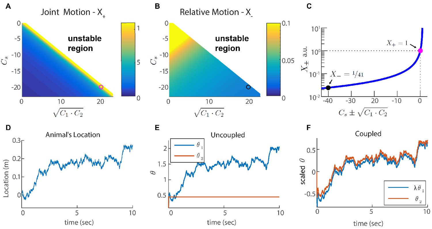
(A-B) Velocity response of the coupled system to velocity inputs that drive joint motion $X_{+}$ . (A) or relative motion $X_{-}$ (B) in two coupled modules, as a function of the coupling strengths. (C) $X_{\pm}$ is a function of one parameter that depends on the coupling strengths ( $C_{s} \pm \sqrt{C_{1} C_{2}}$ ). The magenta and black circles represent the parameters used in (F), and the corresponding value of $X_{+}$ and $X_{-}$ . (D) Simulated trajectory, whose derivative is injected as a velocity input only to module one in panels (E–F). (E) Response of two uncoupled modules ( $C_{1} = C_{2} = C_{s} = 0$ ): the position represented by module 1 tracks the velocity inputs, module 2 is unresponsive, and the updates in the two modules are not coordinated, as expected. (F) Same as (E) but the modules are coupled with coupling strengths: $C_{s} = - 20$ , $C_{1} = - C_{s} / λ ≃ 14.1$ , and $C_{2} = - C_{s} \cdot λ ≃ 28.3$ . The phases of both modules track the velocity inputs in a coordinated manner, with the desirable velocity ratio $λ$ . The phase of module one is scaled by $λ$ ( $λ θ_{1}$ is shown) in order to simplify the comparison between modules.

https://doi.org/10.7554/eLife.48494.004

Figure 4 with 1 supplement

Download asset Open asset

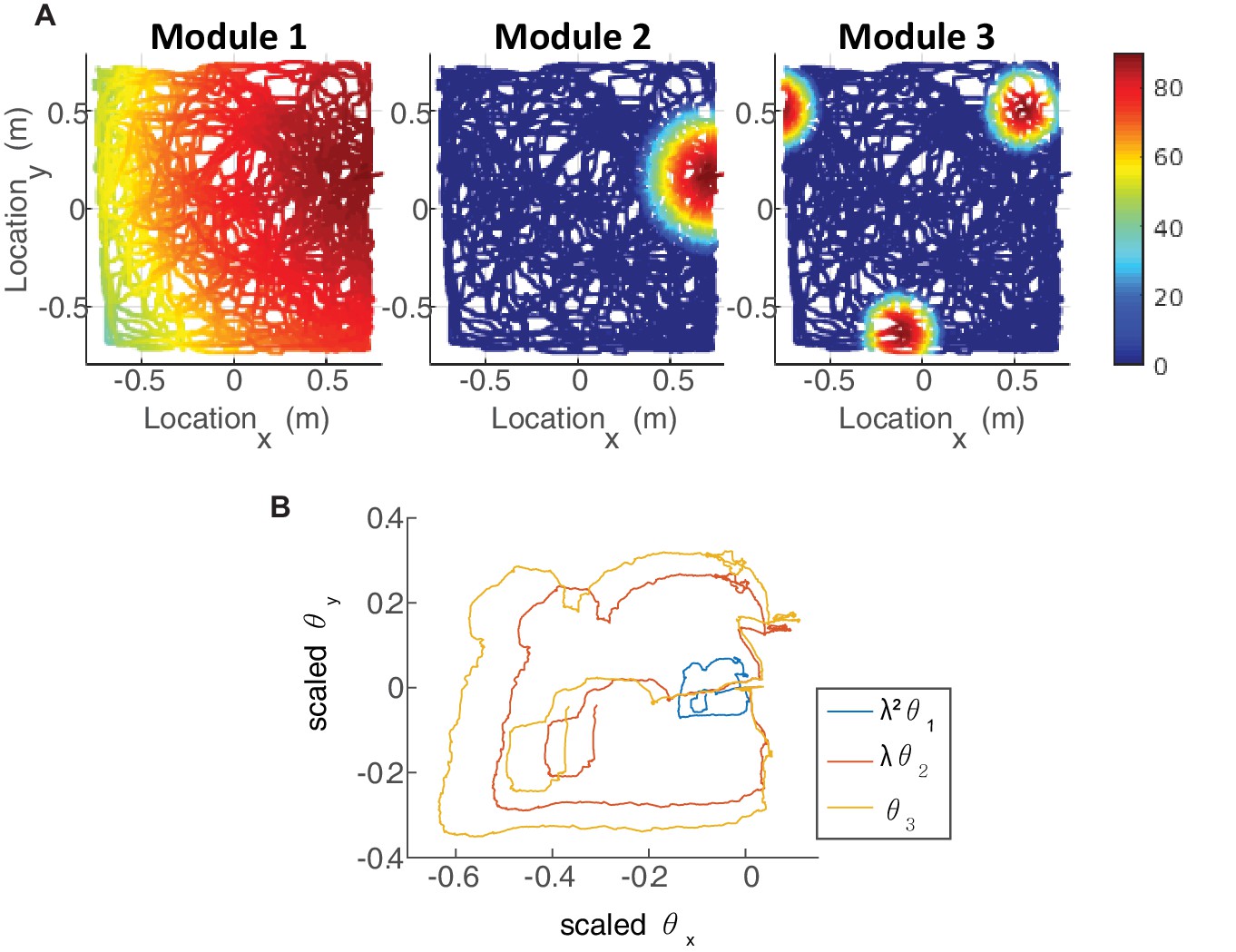
Coupling of several modules in two dimensions.

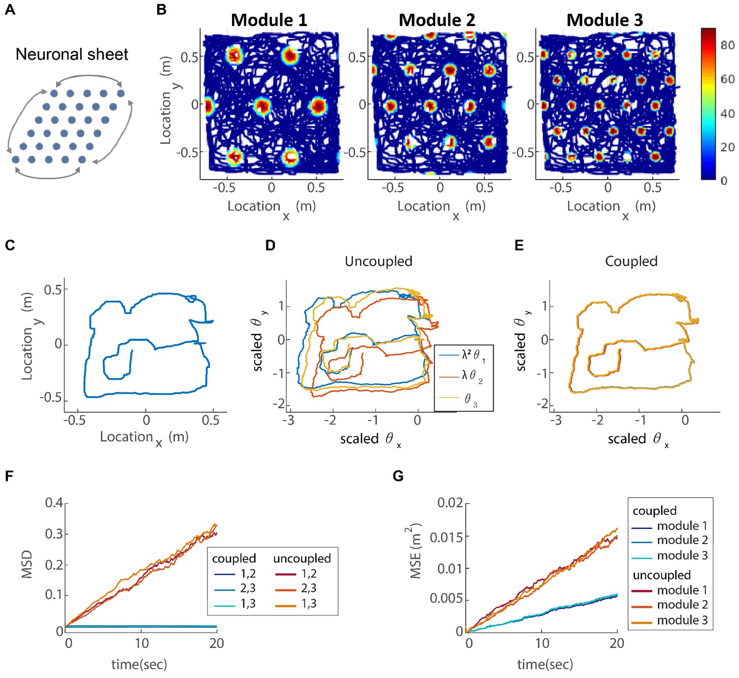
(A) The neurons of each sub-population in the two dimensional case (right, left, up and down) are organized on a neuronal sheet in the shape of a parallelogram with periodic boundary conditions. (B) Simulated firing rate of a single grid cell from each module, as a function of position, evaluated during response of the network to a rat trajectory lasting 800 s (taken from Stensola et al., 2012). (C) Measured rat trajectory over an interval of 20 s (Stensola et al., 2012), whose derivative is injected as a velocity input to all modules in panels (D–E), with addition of uncorrelated noise in each module. (D) Response of three uncoupled modules. (E) Response of three coupled modules. The phases of the three modules approximately track the velocity inputs in both cases, but the coordination between phases of the three modules is more tight in (E). The phases of modules 1 and 2 are scaled by $λ^{2}$ and $λ$ , respectively, in order to simplify the comparison between modules (similar to Figure 3F). (F) Mean square displacement (MSD) between the scaled phases of any two modules over time. Responses of the three modules, as in (D–E), were simulated over a hundred realizations of noise. The mismatch between module trajectories in the coupled case (blue lines) is very small compare to the uncoupled case (red lines). The units of scaled phases are the same as in (D–E). The legend indicates which two module trajectories are compared. (G) Mean square error (MSE) of each module’s trajectory relative to the animal’s trajectory, computed from the same simulations presented in (F). To obtain each module’s trajectory in units of spatial location, the module’s phase was multiplied by its spacing. In the coupled case (blue), the slope of MSE is reduced by a factor of $m = 3$ (the number of modules) compared to the uncoupled case (red), as the noise is averaged due to the coupling.

https://doi.org/10.7554/eLife.48494.005

Figure 4—figure supplement 1

Download asset Open asset

Disconnected module.

Three coupled modules as in Figure 4B,E, but module 1 is disconnected from the other modules, namely $C_{12} = C_{21} = 0$ . All other parameters are identical to Figure 4B,E. (A) Firing rate of a single grid cell from each module. The spacing of all modules increases as expected (compare to Figure 4B and see Discussion). (B) Response of three modules. The scales of phases are not coordinated, thus the spacing ratios change as well. The velocity of phases in response to the same animal’s trajectory is much smaller (see scale of axes in panel B, in comparison to Figure 4E), which indicates larger spacings.

https://doi.org/10.7554/eLife.48494.006

Figure 5 with 2 supplements

Download asset Open asset

Reilience of the spatial representation to noise in velocity inputs.

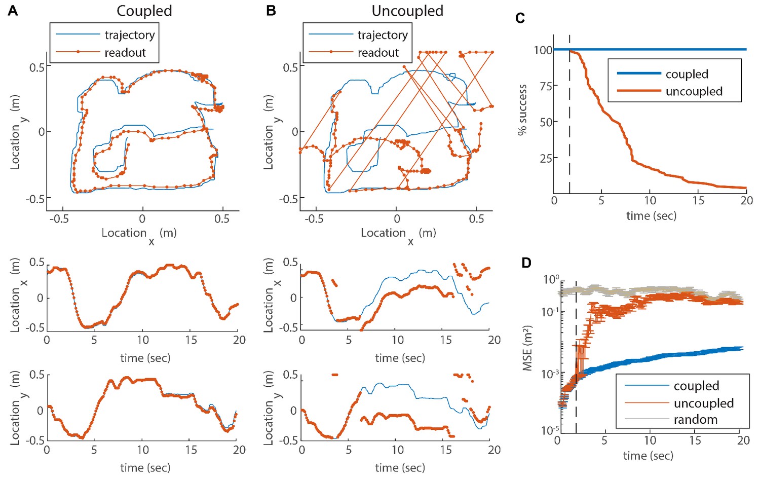
(A) Blue trace: measured rat trajectory over a 20 s interval (taken from Stensola et al., 2012), used as a velocity input to three coupled modules. Red trace: readout of position, decoded from simulated Poisson spikes of the coupled system. The spikes are generated by a Poisson process from the instantaneous firing rates of all cells in the three modules (see Materials and methods). Top panel: the trajectory in the two-dimensional arena. Lower panels: $x$ and $y$ components of the trajectory as a function of time. The decoded position is continuous and similar to the input trajectory. (B) Same as (A), but in a network consisting of three uncoupled modules: all coupling strengths are set to zero. The decoded position is discontinuous in time, and often sharply deviates from the input trajectory. (C) Percentage of decoding success over time. We repeated the decoding of the animal’s trajectory, as in (A–B), over a hundred simulations with different realizations of the noise. A success at time $t$ is defined as a trial that did not contain any discontinuity in the readout up to that time. The success percentage was computed by counting the number of trials without discontinuities at each time point. The coupled network maintains 100% success over time (blue), whereas the success percentage of the uncoupled network decreases significantly over time: many trials contain discontinuities after a few seconds, and almost all of them contain discontinuities after 20 s (red). (D) Mean square error (MSE) of the decoded trajectory, computed from the same simulations presented in (C), in the coupled (blue) and uncoupled (red) cases. Gray trace: MSE computed by random guessing of location. The vertical black dashed line in (C–D) represents the first time in which a discontinuity was observed in any of the trials of the uncoupled network. From this time point onward, the percentage of success of the uncoupled network descends, and the MSE sharply increases (note the logarithmic vertical scale).

https://doi.org/10.7554/eLife.48494.007

Figure 5—figure supplement 1

Download asset Open asset

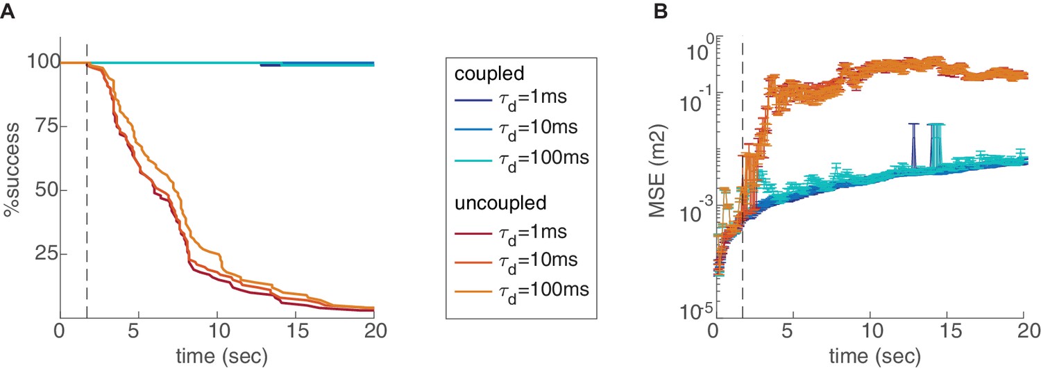
Effect of the readout integration time scale.

Percentage of decoding success (A) and MSE (B) over time, in the coupled (blue) and uncoupled (red) networks, with varying time scales of temporal integration used in the decoding process. Figure 5—figure supplement 2. Effect of the number of modules and environment size. Percentage of decoding success (A,C,E,F,G) and MSE (B,D,H,I,J) as a function of time. (A-D) Varying number of modules ( $m = 3$ , $4$ , or $5$ ), in the coupled (A–B) and uncoupled (C–D) networks. The coupling prevents the occurrence of readout discontinuities in all of these cases. Increase in the number of modules reduces the rate of these discontinuities even in the absence of coupling (C–D). (E-J) Decoding in arena of dimensions 2.5 × 2.5 m₂ (red), compared to the original arena (blue, 1.2 × 1.2 m₂), without coupling and with different number of modules. The rate of readout discontinuities increases, and the MSE increases, in larger arenas.

https://doi.org/10.7554/eLife.48494.008

Figure 5—figure supplement 2

Download asset Open asset

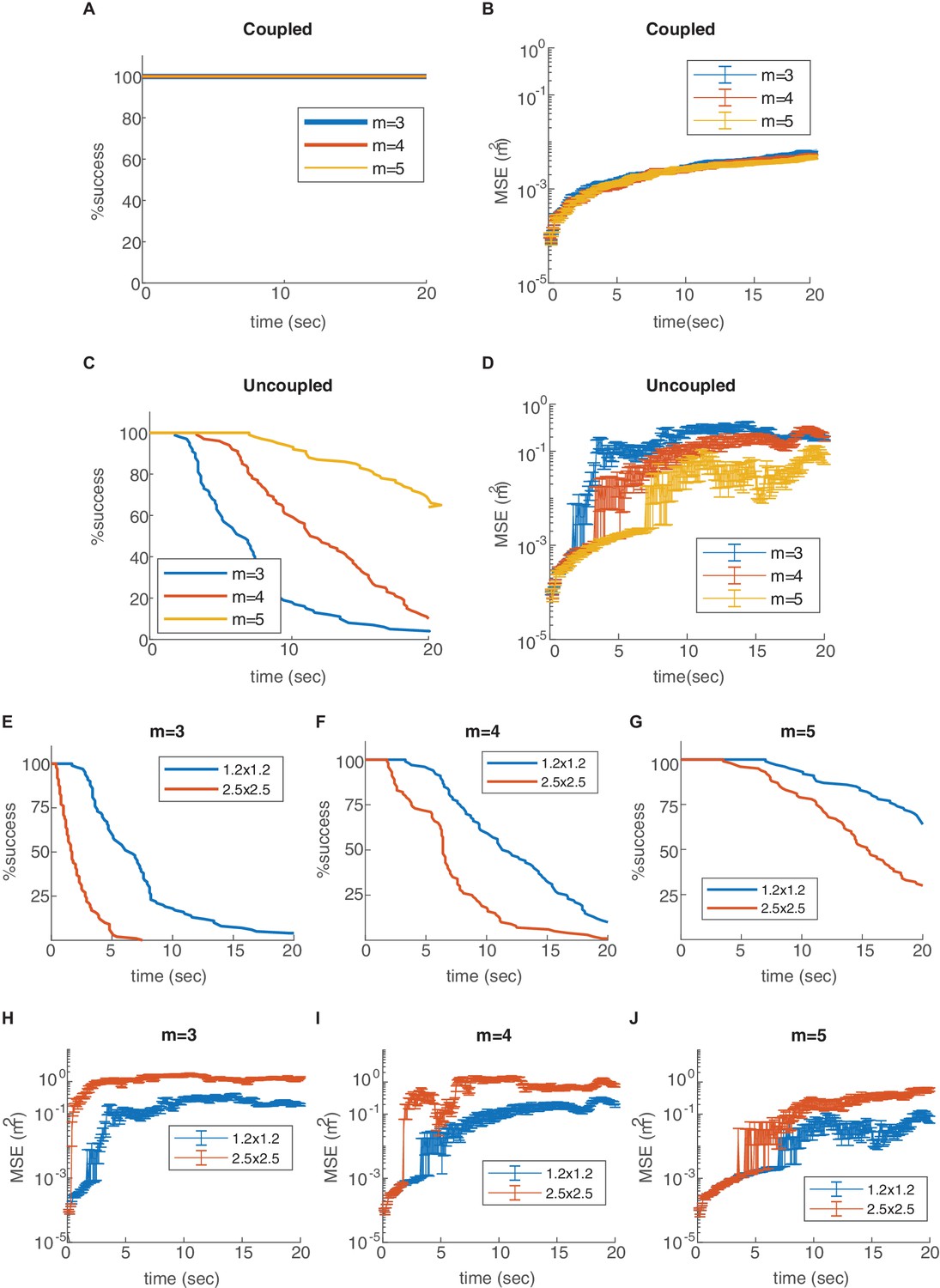
Effect of the number of modules and environment size.

Percentage of decoding success (A,C,E,F,G) and MSE (B,D,H,I,J) as a function of time. (A-D) Varying number of modules ( $m = 3$ , $4$ , or $5$ ), in the coupled (A–B) and uncoupled (C–D) networks. The coupling prevents the occurrence of readout discontinuities in all of these cases. Increase in the number of modules reduces the rate of these discontinuities even in the absence of coupling (C–D). (E-J) Decoding in arena of dimensions 2.5 × 2.5 m₂ (red), compared to the original arena (blue, 1.2 × 1.2 m₂), without coupling and with different number of modules. The rate of readout discontinuities increases, and the MSE increases, in larger arenas.

https://doi.org/10.7554/eLife.48494.009

Figure 6

Download asset Open asset

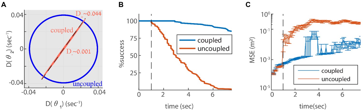
Reilience of the spatial representation to intrinsic neural stochasticity.

(A) Diffusion tensor of a Poisson spiking neural network, consisting of two modules in one dimension, computed using Equation 25, and illustrated as an ellipse. Axes of the ellipse are aligned with the eigenvectors of the diffusion tensor, and the lengths of each axis represents the diffusion coefficient along the corresponding direction. Without coupling the diffusion tensor is isotropic (blue circle). When coupling the modules using the same coupling strengths as in Figure 3F, the diffusion tensor becomes highly anisotropic (red ellipse). The diffusion in this case is almost exclusively in the direction of the first principal component (major axis of the ellipse). This direction closely matches the direction of coordinated drift ( ${\vec{u}}_{+}$ in Equation 55, dashed line). (B-C) same as Figure 5C–D, but for the internal noise case.

https://doi.org/10.7554/eLife.48494.010

Appendix 1—figure 1

Download asset Open asset

Structure of the left null eigenvector.

(A) The left eigenvector of $K$ with zero eigenvalue, $\vec{v} (θ = 0.5)$ (the bump is centered around $θ = 0.5$ ), computed numerically. The first $N$ coordinates of $\vec{v}$ (right sub-population) in red, and the last $N$ coordinates of $\vec{v}$ (left sub-population) in blue. (B) ${\vec{v}}_{-}$ (red and blue for the right and left sub-population respectively), and ${\vec{v}}_{+}$ (yellow, identical for both of the sub-populations), as defined in Equation 41. The black dashed line represents the firing rate bump of the steady state (unitless for the sake of comparison with $\vec{v}$ ).

https://doi.org/10.7554/eLife.48494.013

Additional files

Transparent reporting form: https://doi.org/10.7554/eLife.48494.011
Download elife-48494-transrepform-v2.pdf

Download links

A two-part list of links to download the article, or parts of the article, in various formats.

Downloads (link to download the article as PDF)

Open citations (links to open the citations from this article in various online reference manager services)

Mendeley

Cite this article (links to download the citations from this article in formats compatible with various reference manager tools)

Noga Mosheiff
Yoram Burak

(2019)

Velocity coupling of grid cell modules enables stable embedding of a low dimensional variable in a high dimensional neural attractor

eLife 8:e48494.

https://doi.org/10.7554/eLife.48494

Sign up for email alerts

Privacy notice