DeepFly3D, a deep learning-based approach for 3D limb and appendage tracking in tethered, adult Drosophila
- EPFL, Switzerland
- UBC, Canada
Figures
Figure 1 with 1 supplement
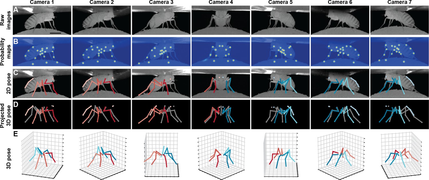
Deriving 3D pose from multiple camera views.
(A) Raw image inputs to the Stacked Hourglass deep network. (B) Probability maps output from the trained deep network. For visualization purposes, multiple probability maps have been overlaid for each camera view. (C) 2D pose estimates from the Stacked Hourglass deep network after applying pictorial structures and multi-view algorithms. (D) 3D pose derived from combining multiple camera views. For visualization purposes, 3D pose has been projected onto the original 2D camera perspectives. (E) 3D pose rendered in 3D coordinates. Immobile thorax-coxa joints and antennal joints have been removed for clarity.
Figure 1—video 1
Deriving 3D pose from multiple camera views during backward walking in an optogenetically stimulated MDN>CsChrimson fly.
https://doi.org/10.7554/eLife.48571.003
Figure 2
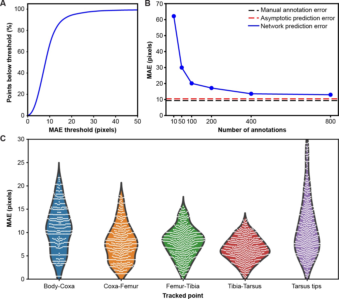
Mean absolute error distribution.
(A) PCK (percentage of keypoints) accuracy as a function of mean absolute error (MAE) threshold. (B) Evaluating network prediction error in a low data regime. The Stacked Hourglass network (blue circles) shows near asymptotic prediction error (red dashed line), even when trained with only 400 annotated images. After 800 annotations, there are minimal improvements to the MAE. (C) MAE for different limb landmarks. Violin plots are overlaid with raw data points (white circles).
Figure 3
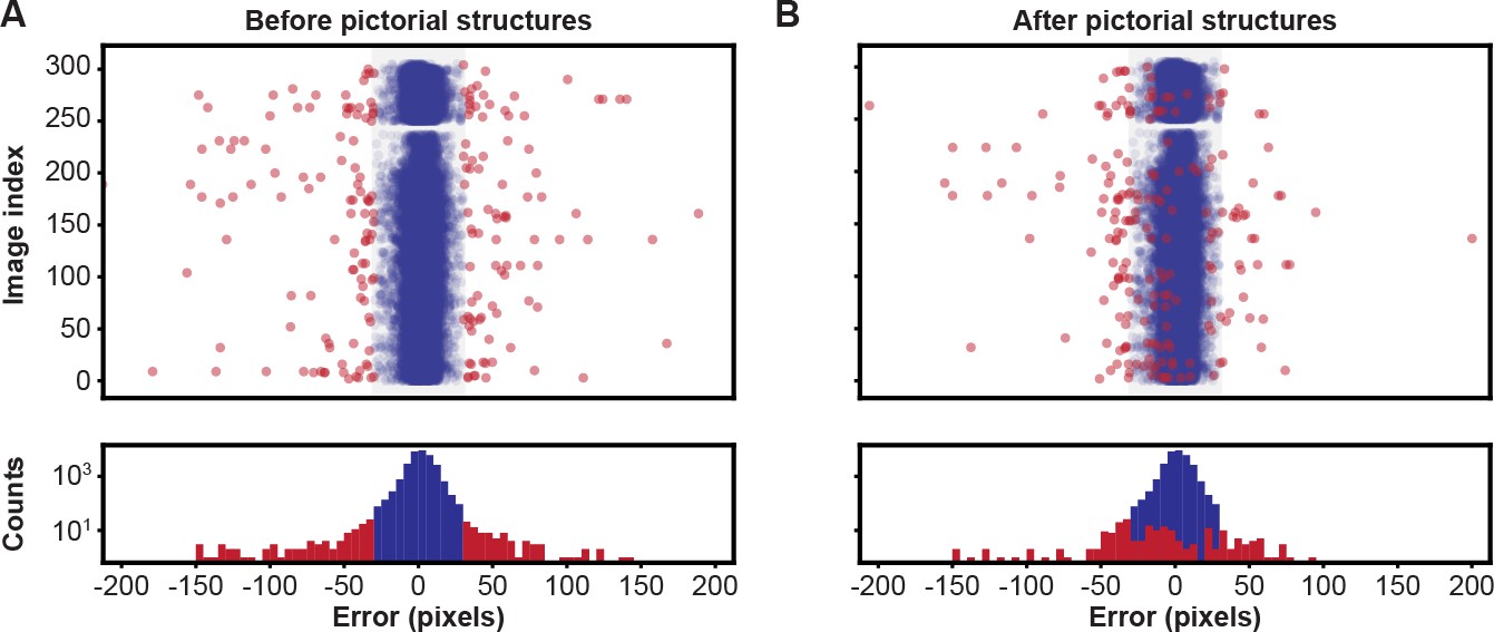
Pose estimation accuracy before and after using pictorial structures.
Pixel-wise 2D pose errors/residuals (top) and their respective distributions (bottom) (A) before, or (B) after applying pictorial structures. Residuals larger than 35 pixels (red circles) represent incorrect keypoint detections. Those below this threshold (blue circles) represent correct keypoint detections.
Figure 4
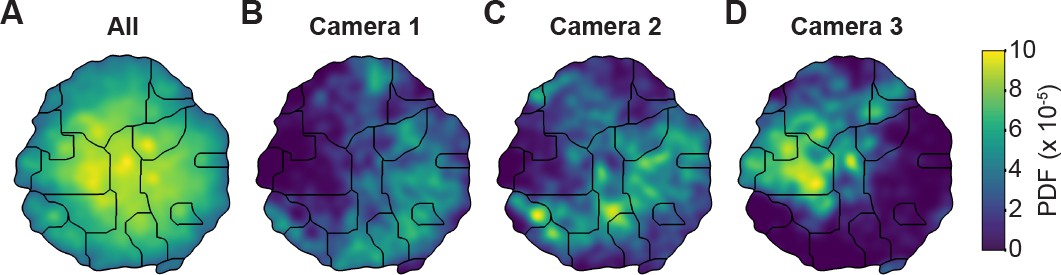
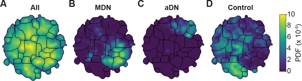
Unsupervised behavioral classification of 2D pose data is sensitive to viewing angle.
(A) Behavioral map derived using 2D pose data from three adjacent cameras (Cameras 1, 2, and 3) but the same animals and experimental time points. Shown are clusters (black outlines) that are enriched (yellow), or sparsely populated (blue) with data. Different clusters are enriched for data from either (B) camera 1, (C) camera 2, or (D) camera 3. Behavioral embeddings were derived using 1 million frames during 4 s of optogenetic stimulation of MDN>CsChrimson (n = 6 flies, n = 29 trials), aDN>CsChrimson (n = 6 flies, n = 30 trials), and wild-type control animals (MDN-GAL4/+: n = 4 flies, n = 20 trials. aDN-GAL4/+: n = 4 flies, n = 23 trials).
Figure 5 with 6 supplements
Unsupervised behavioral classification of 3D joint angle data.
Behavioral embeddings were calculated using 3D joint angles from the same 1 million frames used in Figure 4A. (A) Behavioral map combining all data during 4 s of optogenetic stimulation of MDN>CsChrimson (n = 6 flies, n = 29 trials), aDN>CsChrimson (n = 6 flies, n = 30 trials), and wild-type control animals (For MDN-Gal4/+, n = 4 flies, n = 20 trials. For aDN-Gal4/+ n = 4 flies, n = 23 trials). The same behavioral map is shown with only the data from (B) MDN>CsChrimson stimulation, (C) aDN>CsChrimson stimulation, or (D) control animal stimulation. Associated videos reveal that these distinct map regions are enriched for backward walking, antennal grooming, and forward walking, respectively.
Figure 5—video 1
Representative MDN>CsChrimson optogenetically activated backward walking. Orange circle indicates LED illumination and CsChrimson activation.
https://doi.org/10.7554/eLife.48571.008
Figure 5—video 2
Representative aDN>CsChrimson optogenetically activated antennal grooming. Orange circle indicates LED illumination and CsChrimson activation.
https://doi.org/10.7554/eLife.48571.009
Figure 5—video 3
Representative control animal behavior during illumination. Orange circle indicates LED illumination and CsChrimson activation.
https://doi.org/10.7554/eLife.48571.010
Figure 5—video 4
Sample behaviors from 3D pose cluster enriched in backward walking.
https://doi.org/10.7554/eLife.48571.011
Figure 5—video 5
Sample behaviors from 3D pose cluster enriched in antennal grooming.
https://doi.org/10.7554/eLife.48571.012
Figure 5—video 6
Sample behaviors from 3D pose cluster enriched in forward walking.
https://doi.org/10.7554/eLife.48571.013
Figure 6
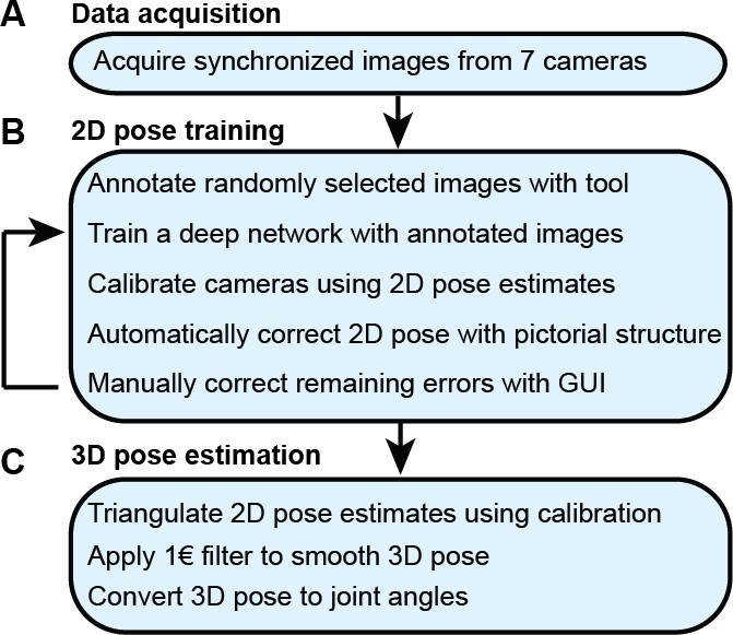
The DeepFly3D pose estimation pipeline.
(A) Data acquisition from the multi-camera system. (B) Training and retraining of 2D pose. (C) 3D pose estimation.
Figure 7
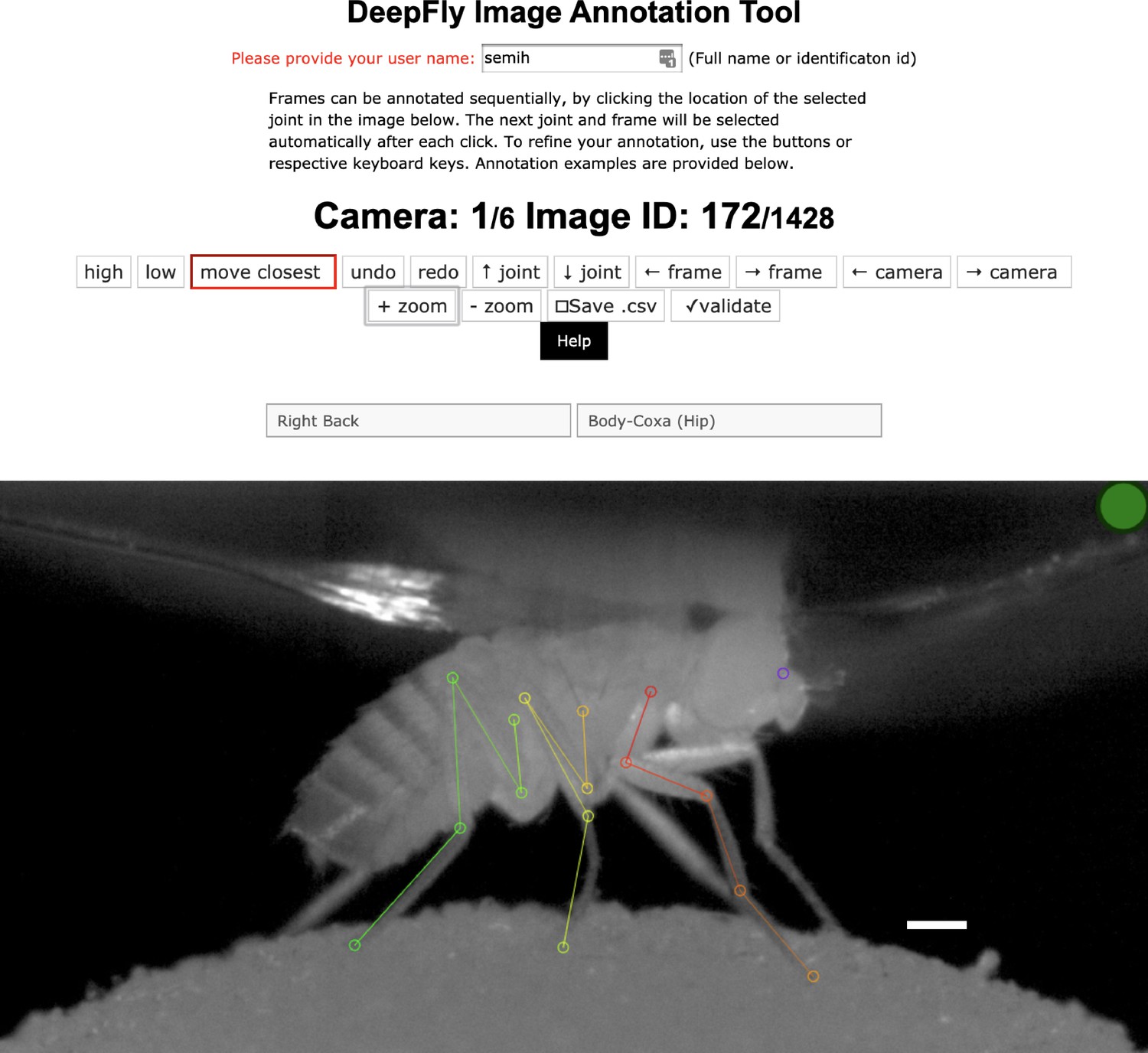
The DeepFly3D annotation tool.
This GUI allows the user to manually annotate joint positions on images from each of seven cameras. Because this tool can be accessed from a web browser, annotations can be performed in a distributed manner across multiple users more easily. A full description of the annotation tool can be found in the online documentation: https://github.com/NeLy-EPFL/DeepFly3D. Scale bar is 50 pixels.
Figure 8

Camera calibration.
(A) Correcting erroneous 2D pose estimations by using epipolar relationships. Only 2D pose estimates without large epipolar errors are used for calibration. represents a 2D pose estimate from the middle camera. Epipolar lines are indicated as blue and red lines on the image plane. (B) The triangulated point, , uses the initial camera parameters. However, due to the coarse initialization of each camera’s extrinsic properties, observations from each camera do not agree with one another and do not yield a reasonable 3D position estimate. (C) The camera locations are corrected, generating an accurate 3D position estimate by optimizing Equation 7 using only the pruned 2D points.
Figure 9

3D pose correction for one leg using the MAP solution and pictorial structures.
(A) Candidate 3D pose estimates for each keypoint are created by triangulating local maxima from probability maps generated by the Stacked Hourglass deep network. (B) For a selection of these candidate estimates, we can assign a probability using Equation 8. However, calculating this probability for each pair of points is computationally intractable. (C) By exploiting the chain structure of Equation 8, we can instead pass a probability distribution across layers using a belief propagation algorithm. Messages are passed between layers as a function of parent nodes, describing the belief of the child nodes on each parent node. Grayscale colors represent the calculated belief of each node where darker colors indicate higher belief. (D) Corrected pose estimates are obtained during the second backward iteration, by selecting the nodes with largest belief. We discard nodes (x’s) that have non-maximal belief during backwards message passing. Note that beliefs have been adjusted after forward message passing.
Figure 10
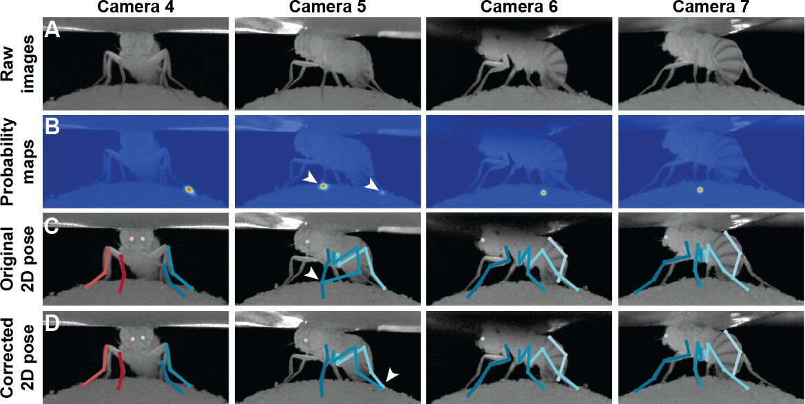
Pose correction using pictorial structures.
(A) Raw input data from four cameras, focusing on the pretarsus of the middle left leg. (B) Probability maps for the pretarsus output from the Stacked Hourglass deep network. Two maxima (white arrowheads) are present on the probability maps for camera 5. The false-positive has a larger unary probability. (C) Raw predictions of 2D pose estimation without using pictorial structures. The pretarsus label is incorrectly applied (white arrowhead) in camera 5. By contrast, cameras 4, 6, and 7 are correctly labeled. (D) Corrected pose estimation using pictorial structures. The false-positive is removed due to the high error measured in Equation 8. The newly corrected pretarsus label for camera five is shown (white arrowhead).
Figure 11
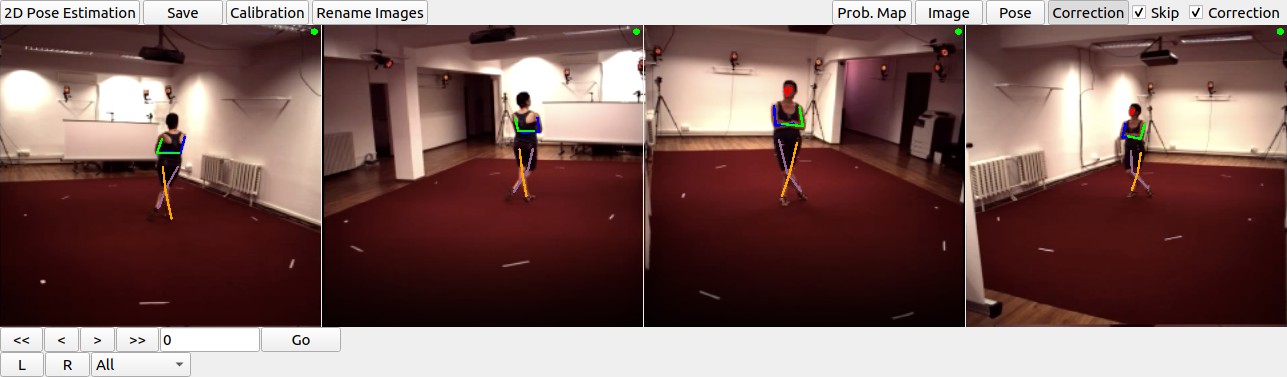
DeepFly3D graphical user interface (GUI) applied to with the Human3.6M dataset (Ionescu et al., 2014).
To use the DeepFly3D GUI on any new dataset (Drosophila or otherwise), users can provide an initial small set of manual annotations. Using these annotations, the software calculates the epipolar geometry, performs camera calibration, and trains the 2D pose estimation deep network. A description of how to adopt DeepFly3D for new datasets can be found in the Materials and methods section and, in greater detail, online: https://github.com/NeLy-EPFL/DeepFly3D. This figure is licensed for academic use only and thus is not available under CC-BY and is exempt from the CC-BY 4.0 license.
Figure 12
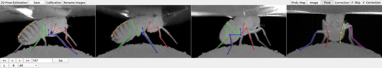
DeepFly3D graphical user interface (GUI).
The top-left buttons enable operations like 2D pose estimation, camera calibration, and saving the final results. The top-right buttons can be used to visualize the data in different ways: as raw images, probability maps, 2D pose, or the corrected pose following pictorial structures. The bottom-left buttons permit frame-by-frame navigation. A full description of the GUI can be found in the online documentation: https://github.com/NeLy-EPFL/DeepFly3D.
Figure 13
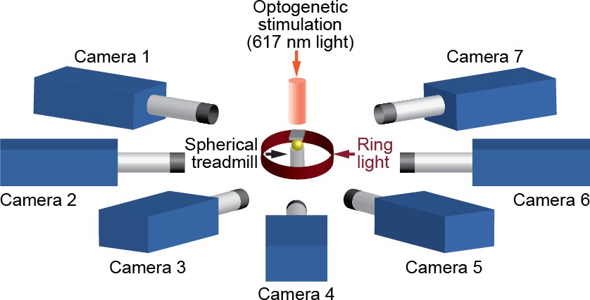
A schematic of the seven camera spherical treadmill and optogenetic stimulation system that was used in this study.
https://doi.org/10.7554/eLife.48571.021
Author response image 1
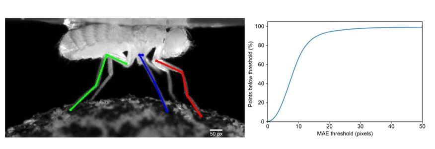
Interpreting and choosing the PCK Threshold.
(a) An illustration of the length of the PCK (percentage of keypoints) error threshold (Scale bar, bottom right) for comparison with limb segment lengths. The 50 pixel threshold is approximately one-third the length of the prothoracic femur. (b) PCK accuracy as a function of mean absolute error (MAE) threshold.
Author response image 2
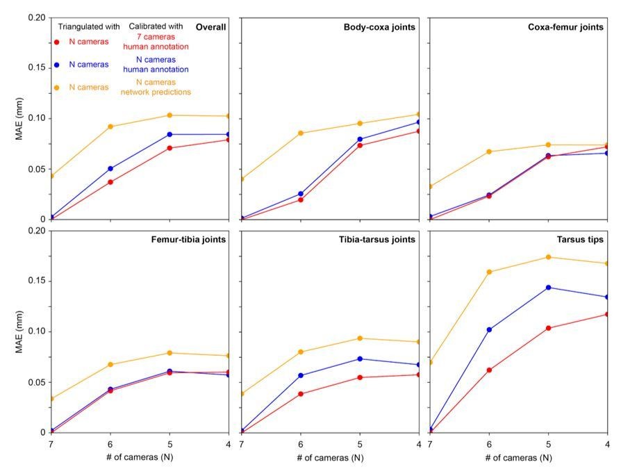
Triangulation error for each joint as a function of number of cameras used for calibration.
Mean absolute error (MAE) as a function of number of cameras used for triangulation and calibration, as well as human annotation versus network prediction. Calibration using all 7 cameras and human annotation is the ground truth (red circles). This ground truth is compared with using N cameras for triangulation and performing calibration from N cameras using either human annotation of images (blue circles) or network predictions of images (yellow circles). A comparison across joints (individual panels) demonstrates that certain joints (e.g., tarsus tips) are more susceptible to increased errors with fewer cameras.
Author response image 3
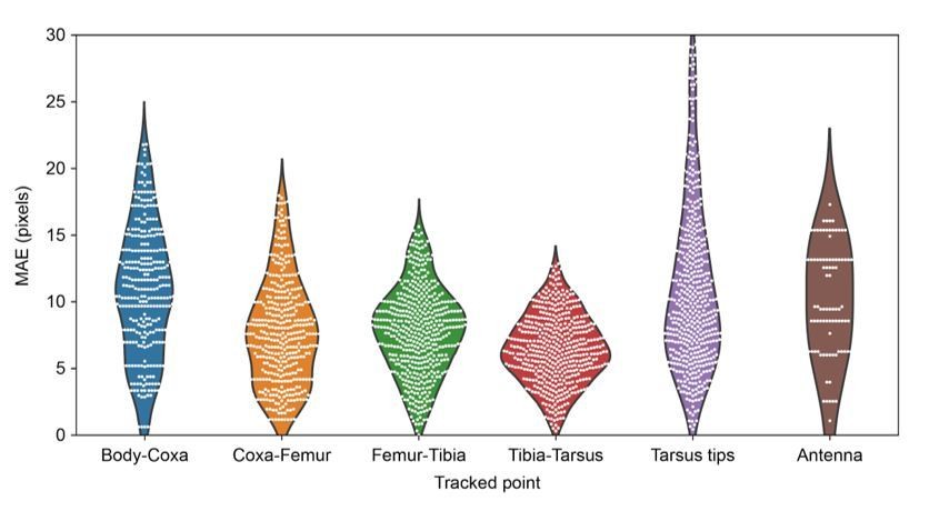
MAE errors for limb and antennal landmarks.
MAE as a function of landmark showing the differential distribution of errors. Violin plots are overlaid with raw data points (white circles).
Additional files
-
Transparent reporting form
- https://doi.org/10.7554/eLife.48571.022
Download links
A two-part list of links to download the article, or parts of the article, in various formats.
Downloads (link to download the article as PDF)
Open citations (links to open the citations from this article in various online reference manager services)
Cite this article (links to download the citations from this article in formats compatible with various reference manager tools)
DeepFly3D, a deep learning-based approach for 3D limb and appendage tracking in tethered, adult Drosophila
eLife 8:e48571.
https://doi.org/10.7554/eLife.48571


