Motor cortex can directly drive the globus pallidus neurons in a projection neuron type-dependent manner in the rat
- Doshisha University, Japan
- National Institute for Physiological Sciences, Japan
Figures
Figure 1 with 3 supplements
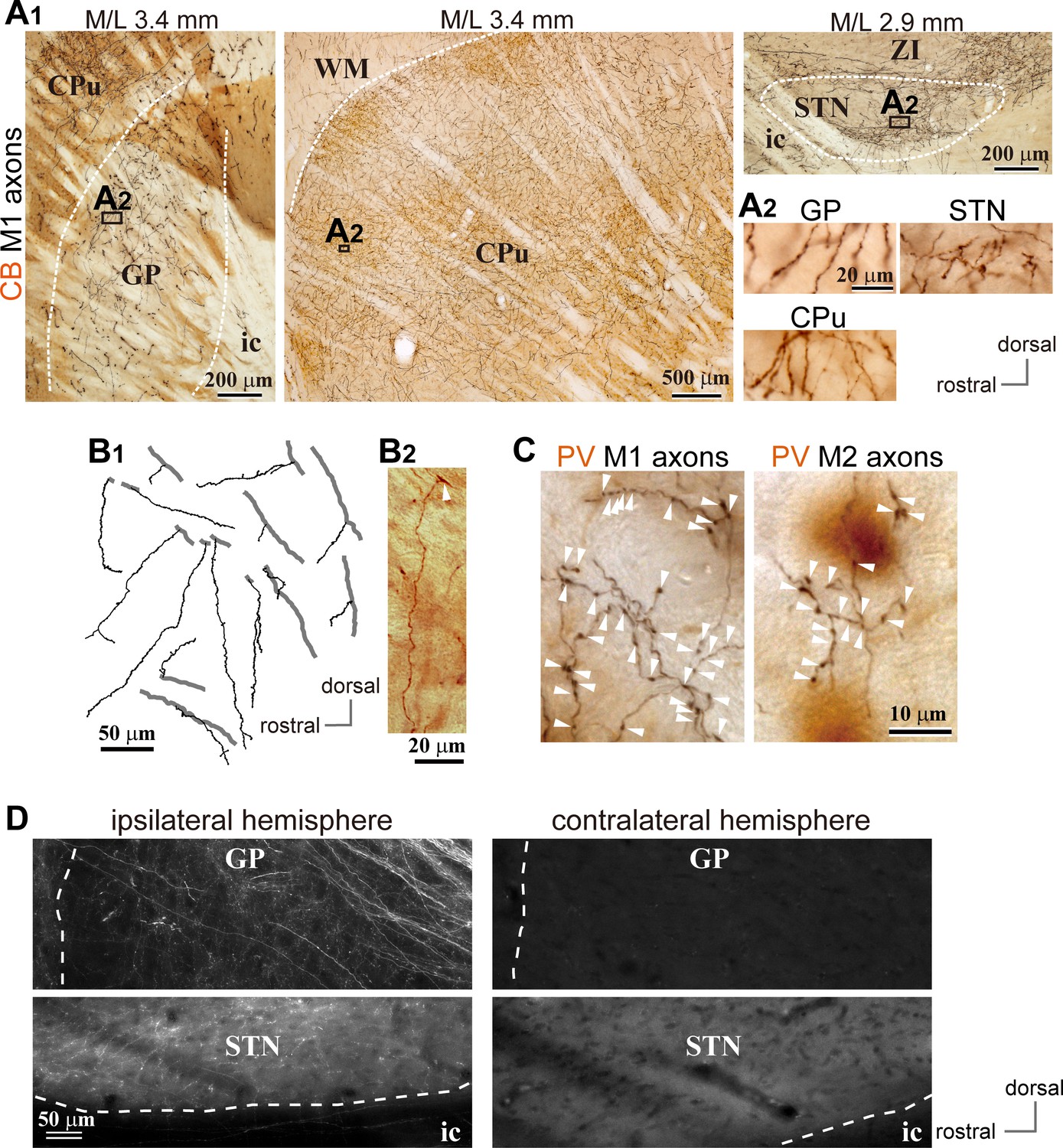
Motor cortical axons project to the globus pallidus (GP).
(A) Representative images of axons in the GP, striatum, and STN originated from the primary motor cortex (M1), labeled with biotinylated dextran amine (BDA; visualized in black). Cortical axons in the GP are predominantly distributed in the calbindin (CB)-negative regions. CB is visualized in brown. Irrespective of differences in axon density among the GP, striatum, and STN, the morphology of the axons and varicosities is similar (A2). (B) Drawings and an image of cortical axons in the GP. The collaterals (thin black lines in B1) were issued from thick axon trunks (thick gray lines in B1; arrowhead in B2). (C) Magnified views of cortical axon varicosities (arrowheads) in the GP; left, M1 axons; right, M2 axons. The images are composites from multiple focal planes. The sections were counter-stained with an anti-parvalbumin (PV) antibody, visualized in brown. (D), Cortical axons in the GP were found exclusively in the ipsilateral hemisphere. M2 axons were visualized with AAV. Similar to axons in the STN, fluorescent signals were not detected in the contralateral GP even by over-exposure.
Figure 1—figure supplement 1

Example images of M1 projections to the GP, STN, and striatum (related to Figure 1).
(A), Using BDA injections into M1, labeled axons are visualized in black and CB immunoactivity in brown. Axons are distributed in the GP lateral to the midline (M/L 2.9–4.2 mm). (B), In the same specimen, cortical axons in the STN were densely distributed at M/L 2.6 and 2.9 mm. The spatial extent of axons was restricted to the medio-caudal position of the STN. (C), M1 axons in the striatum. Note that the scale is different from A and B. (D), Magnified images of the black rectangle area, which is the ROI used for the axon varicosity count, shown in A, B, and C. Note that the size of the ROI is large enough to sample the densely innervated area.
Figure 1—figure supplement 2
Example images of M2 projections to the GP, striatum, and STN (related to Figure 1).
(A), Using BDA injections into M2, labeled axons are visualized in black and CB immunoactivity in brown. Axons are distributed in the GP (M/L 2.6–3.2 mm). (B), In the same specimen, cortical axons in the STN were densely distributed at M/L 2.4 and 2.6 mm. The spatial extent of axons was restricted to the medio-caudal position of the STN. (C), M2 axon in the striatum. Note that the scale is different from A and B. (D), Magnified images of the black rectangle area, which is the ROI used for the axon varicosity count, shown in A, B, and C. (E), Normalized bouton density in the STN.
Figure 1—figure supplement 3
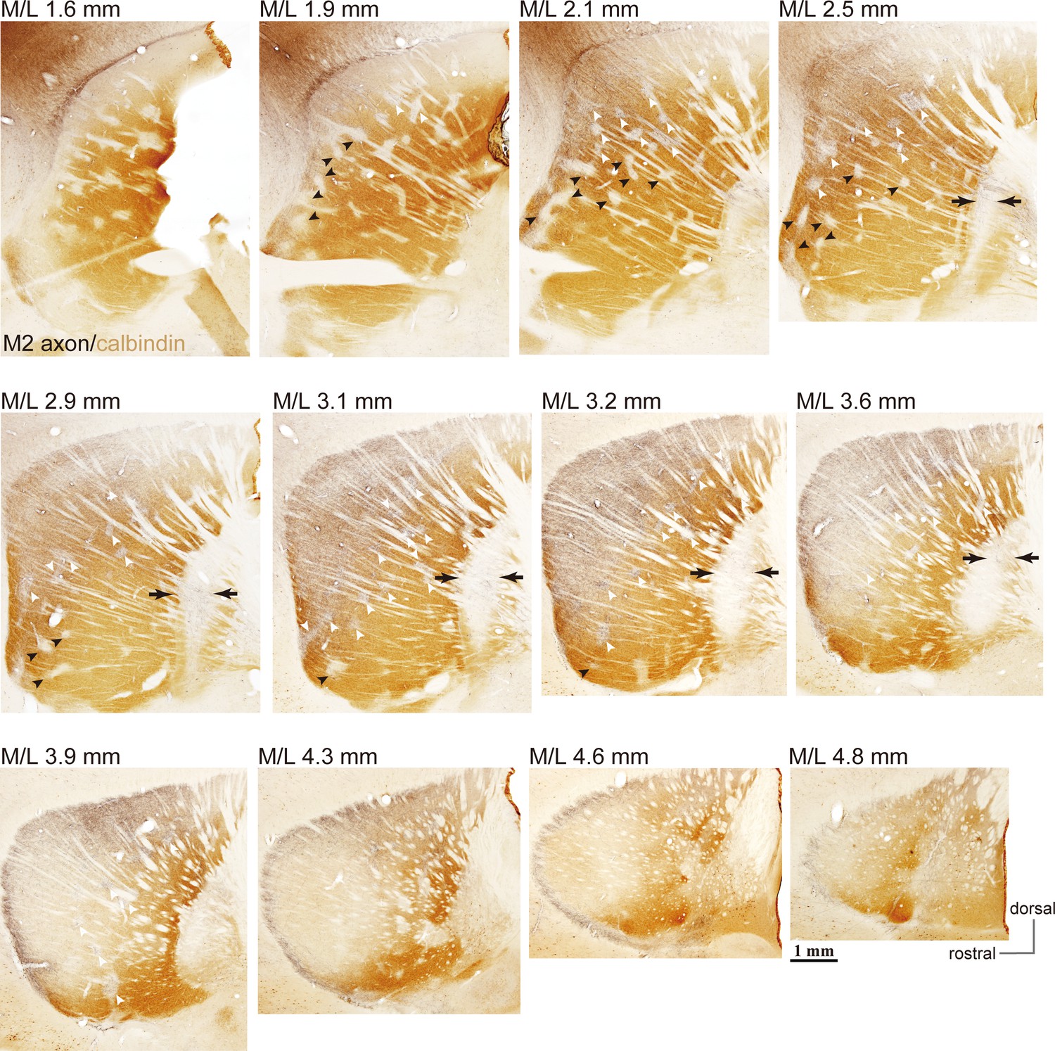
Example images of M2 projections to the striatum and GP (related to Figure 1).
Using BDA injections into M2, labeled axons are visualized in black and CB immunoactivity in brown. Axons are densely distributed in the dorso-lateral striatum (M/L 2.1–4.3 mm). In more lateral sections, axons were denser in CB(-) subregions, and were also found in striosomes [white arrowheads; small CB(-) subregions] throughout the entire projection field. In medial sections, M2 axons were observed in both CB(+) and CB(-) subregions. M2 axons were only faintly detected in ventral striosomes (filled arrowheads), whereas they were relatively dense in dorsal striosomes (white arrowheads). Note also the presence of M2 axons in CB(-) portions of the GP (arrows).
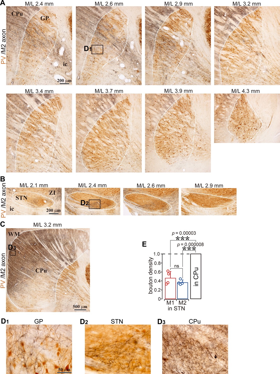
Figure 2 with 2 supplements
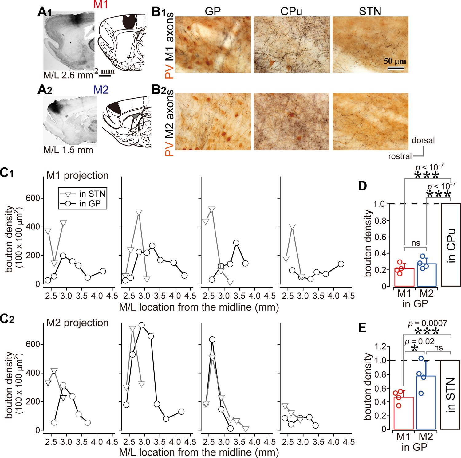
Comparison of axonal bouton density in the GP, striatum, and STN.
(A), Images and drawings of BDA injection sites into the primary and secondary motor areas (M1 and M2, respectively). Tracer was deposited across the entire thickness of the cortex. (B) Images of axon distributions in the GP, striatum, and STN from M1 and M2. To clearly represent axon density, the images are composites from multiple focal planes. (C) Comparison of axon varicosity density in the GP with that in the STN along the M/L dimension (N = 4 animals for each M1 and M2). In most cases, varicosities in the STN showed a sharp peak at a given M/L position. In the GP, M1 axon varicosities were broadly distributed along the M/L dimension. M2 axons tended to be densely distributed in the medial portion. (D) The axon varicosity density in the GP was normalized to that in the striatum or the STN (E).
-
Figure 2—source data 1
Source data for Figure 2C.
- https://doi.org/10.7554/eLife.49511.009
-
Figure 2—source data 2
Source data for Figure 2D and E, Figure 1—figure supplement 2E, and Figure 2—figure supplement 1D.
- https://doi.org/10.7554/eLife.49511.010
Figure 2—figure supplement 1
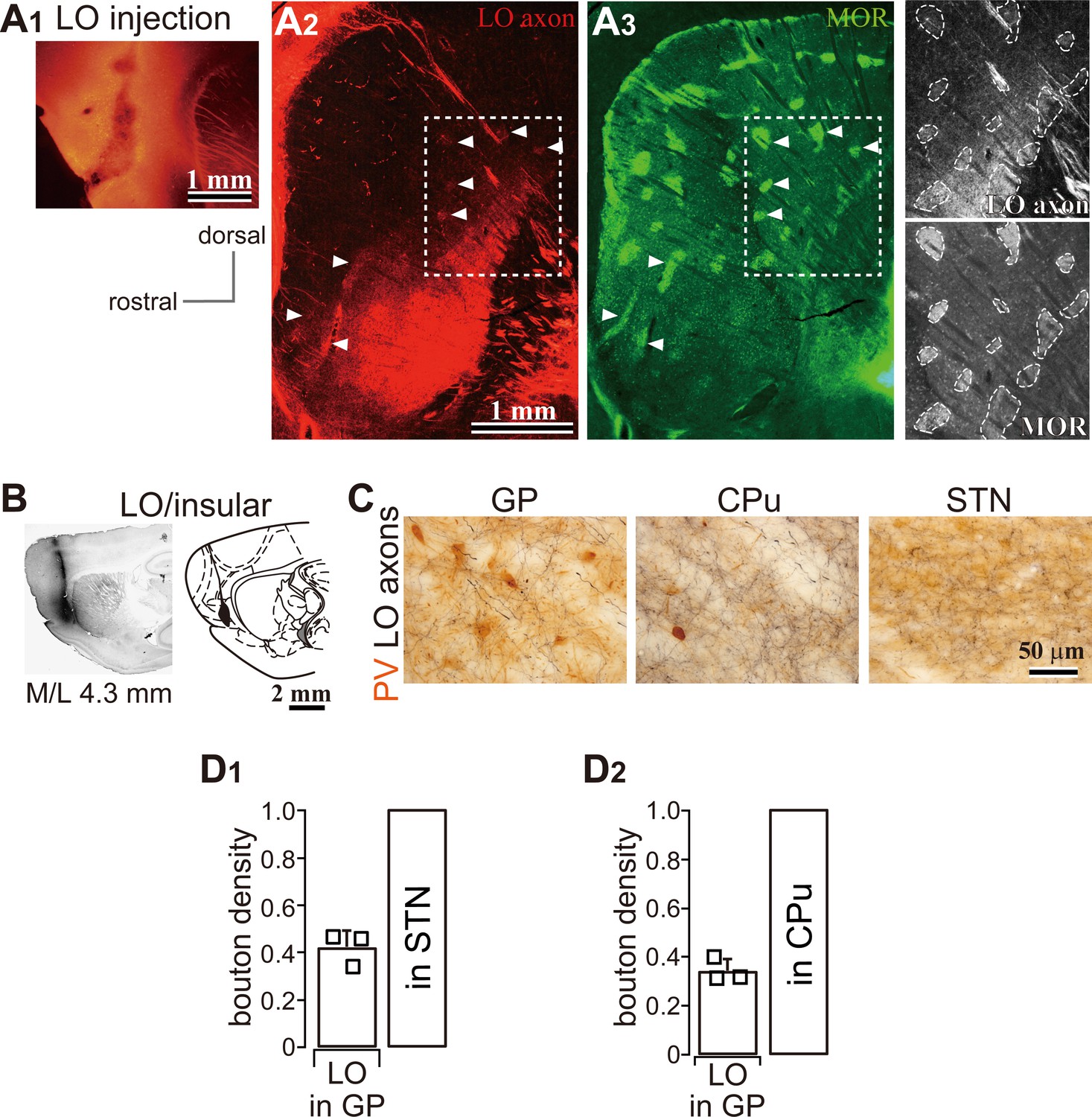
LO projections to the basal ganglia (related to Figure 2).
(A) LO projections to the striatum. (A1) An AAV injection site in the LO. (A2) A representative LO projection to the striatum. LO axons (red) are distributed in the caudal and ventral part of the dorsal striatum (M/L 2.6 mm). (A3) Immunofluorescence for μ-opioid receptor (MOR, green). Arrowheads indicate the striosomes, which are MOR (+), innervated by the LO axons seen in A2 and A3. The square surrounded by a dotted line in A2 and A3 is magnified in the right-most column. (B) BDA injection into the LO. (C) Brightfield images of LO axons in the GP, striatum (CPu), and STN. Note that axon and terminal densities in the GP were lower than those in the striatum or STN. (D) Quantitative comparison of axon density in the GP normalized to that in the STN (D1) and striatum (D2).
Figure 2—figure supplement 2

Cingulate cortex (Cg) projections to the basal ganglia (related to Figure 2).
(A) Cg projections to the striatum (CPu) in sagittal sections (M/L 2.1 mm). Cg axons are dense in the CB-negative subregions of the striatum. Cg axons were less dense in the CB-negative striosomes. (B) Cg projections to the GP. Cg axon collaterals were dense in the CB (-) central GP. Thick axon bundles pass through the dorsal side of the medial GP (M/L 2.4 mm). (C) Cg projections to the STN. Cg axons are localized in the caudal part of the medial STN (arrowheads; M/L 2.4 mm).
Figure 3
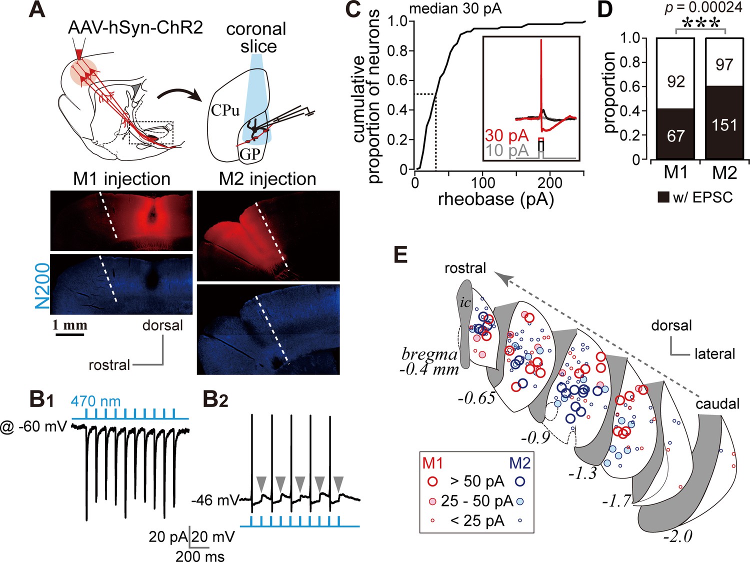
Photoactivation of motor cortical terminals evokes excitation in GP neurons.
(A) Schematic (top) of AAV encoding channelrhodopsin 2 and mCherry injection into the motor cortex for ex vivo recordings using coronal slices. Examples of AAV injection sites are shown in the middle panels (red). Images of immunofluorescence for neurofilament 200 kDa (N200, bottom), used for identification of the M1/M2 border (white dotted lines). (B1) A representative voltage clamp trace (held at −60 mV) showing inward currents in GP neurons elicited by 5 ms blue light pulses (470 nm). (B2) A representative current clamp trace showing photoinduced action potentials and excitatory postsynaptic potentials (EPSPs, arrowheads). (C) Cumulative histogram of the rheobase current of GP neurons. Note that 25 to 30 pA is sufficient to elicit action potentials in half of GP neurons (N = 100). (D) Proportion of GP neurons innervated by M1 or M2 terminals. The number of neurons is shown in bars. M2 more frequently innervated the GP than did M1. (E) Location of GP neurons innervated by M1 (red circle) or M2 (blue circle). Note the topographic distribution of M1 and M2 innervation. The size of circles represents the amplitude of optically evoked currents.
Figure 4
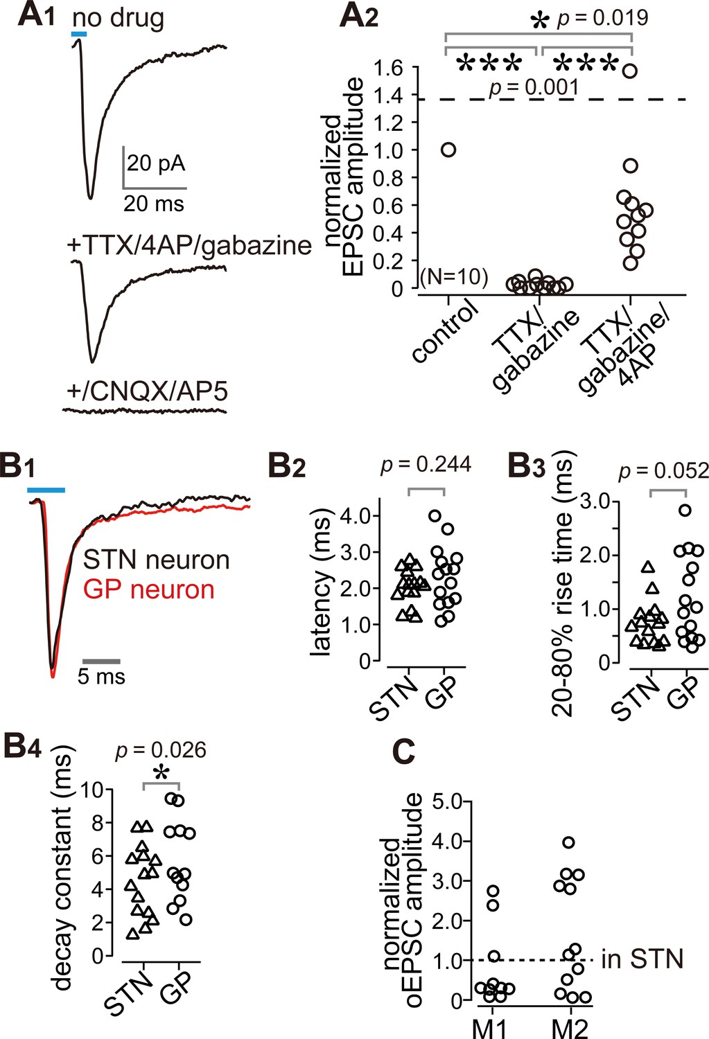
Cortico-pallidal connections are monosynaptic and glutamatergic.
(A) The current induced by optogenetic stimulation of cortical terminals is monosynaptic and glutamatergic. (A1) Representative traces of pharmacological effects on the light-induced inward current. Top, no treatment; Middle, effects of TTX, 4AP, and gabazine; Bottom, effects of additional application of glutamate receptor antagonists (CNQX, AP5). (A2) A summary plot of pharmacological treatments (N = 10 GP neurons). (B) Comparison of the time courses of optogenetically evoked EPSCs (oEPSCs). (B1) Representative traces recorded from STN (black) and GP (red) neurons. The GP and STN neurons were not recorded simultaneously. (B2-4) Summary plots of oEPSC time courses in STN and GP neurons. (B2) The latency from light onset to oEPSC onset does not differ between STN and GP neurons (both N = 15 neurons). The rise time (B3) and the decay constant (B4) of oEPSCs tended to be longer in GP neurons (N = 15 GP neurons and 12 STN neurons). (C), Comparison of oEPSC amplitude between GP and STN neurons, derived from the same animal. The amplitude in the GP neurons was normalized to that in the STN. No significant difference was observed between GP and STN neurons.
-
Figure 4—source data 1
Source data for Figure 4A.
- https://doi.org/10.7554/eLife.49511.014
-
Figure 4—source data 2
Source data for Figure 4B and C.
- https://doi.org/10.7554/eLife.49511.015
Figure 5
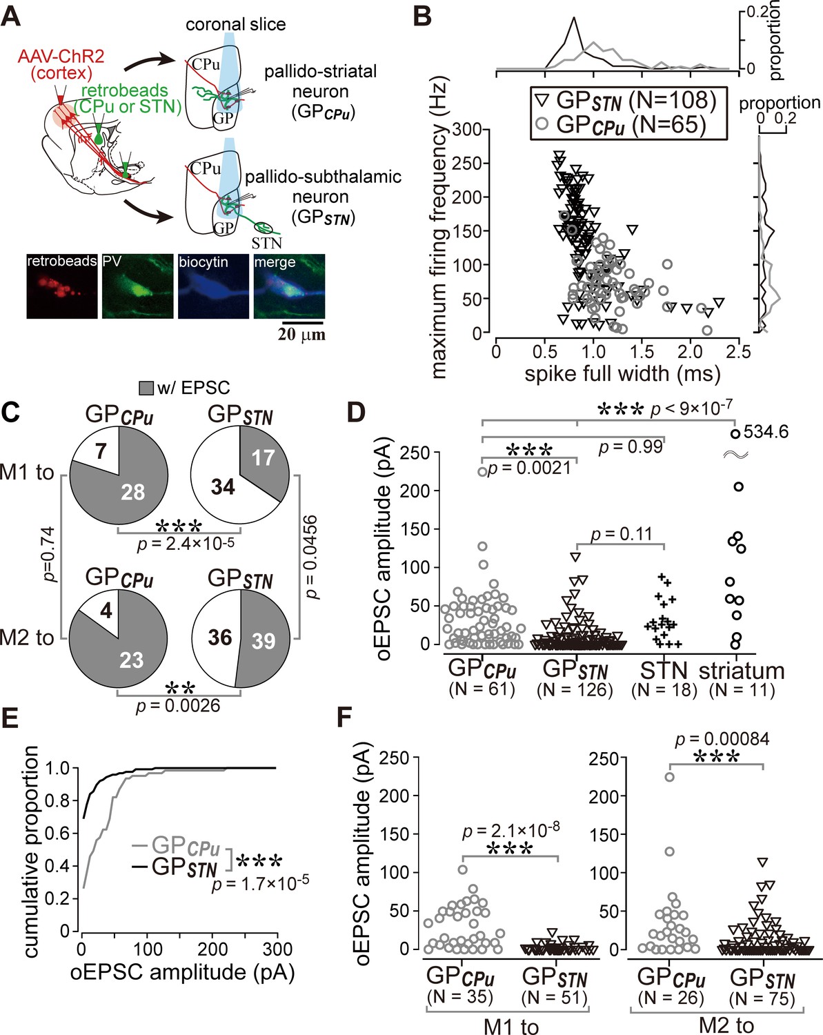
Cell type-dependent cortical innervation of pallidal neurons.
(A) Schematic of ex vivo recordings from retrogradely labeled GP neurons to investigate the effect of GP neuron projection type on cortical innervation. (B) Electrophysiological differences between GP neurons projecting to the striatum (GPCPu) and STN (GPSTN) (see also Table 1). (C) The proportion of GP neurons innervated by M1 or M2 is correlated with projection type. GPCPu neurons were more often innervated by M1 or M2 than GPSTN neurons. Significance was examined using Fisher’s exact test with a Bonferroni correction for multiple comparisons (***, p<0.00025; **, p<0.0025; *, p<0.0125). (D) Amplitudes of oEPSCs in GP, STN, and striatal neurons. The amplitude in GP neurons is similar to that in STN neurons but smaller than that in striatal medium spiny neurons (MSNs). Data obtained from M1 and M2 stimulation are summed. (E) Cumulative histograms of oEPSC amplitude in GPCPu and GPSTN neurons. GPCPu neurons exhibit a greater optically evoked EPSC (oEPSC) amplitude. (F) Left, amplitudes of oEPSCs induced in GP neurons by M1 terminal stimulation. The GPCPu group shows larger oEPSC amplitudes than the GPSTN group. Right, amplitudes of oEPSCs induced by M2 terminal stimulation. Significantly larger oEPSCs were again recorded in the GPCPu group (p=0.00084), but the difference is small.
-
Figure 5—source data 1
Source data for Figure 5B.
The file also contained source data for Table 1.
- https://doi.org/10.7554/eLife.49511.017
-
Figure 5—source data 2
Source data for Figures 5C, D, E and F.
- https://doi.org/10.7554/eLife.49511.018
Figure 6
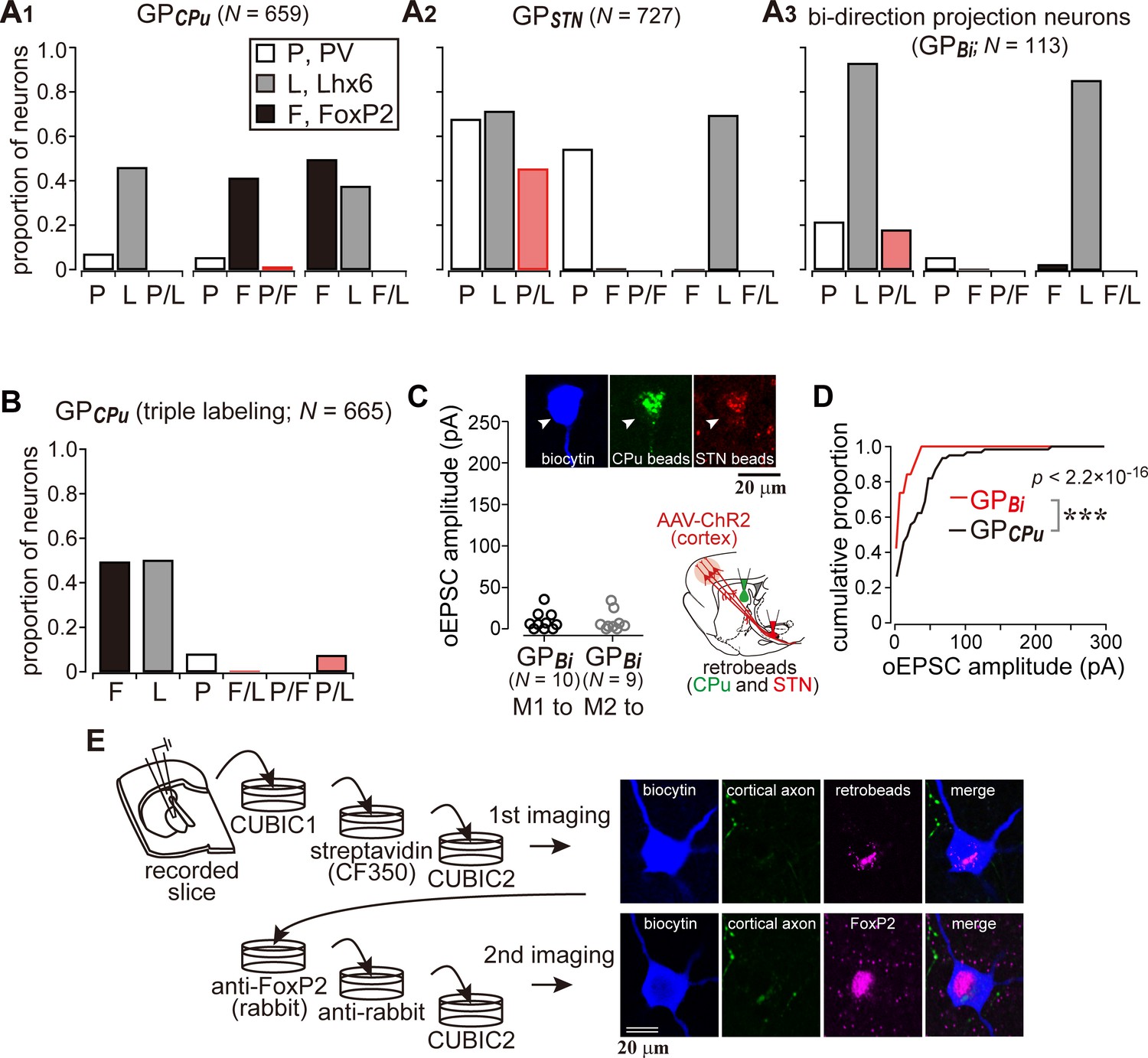
Cortical inputs on bi-directional projection GP neurons (GPBi) and arkypallidal neurons.
Two distinct retrograde tracers were injected into the STN and striatum (CPu), respectively. (A) Three combinations of double immunofluorescence (PV/Lhx6, PV/FoxP2, and Lhx6/FoxP2) were applied. CPu-projecting GP neurons (GPCPu) expressed either FoxP2 or Lhx6 exclusively (A1), whereas STN-projecting GP neurons (GPSTN) were mainly composed of PV- and/or Lhx6-expressing neurons (A2). (A3) GP neurons projecting to both the CPu and STN (GPBi) frequently expressed Lhx6, but not FoxP2. (B) Triple immunofluorescence for GPCPu neurons. Only a single retrograde tracer was injected into the striatum. (C) oEPSC amplitudes of GPBi neurons. Most GPBi neurons exhibited small amplitudes of oEPSCs. Green and red retrobeads were injected into the CPu and STN, respectively. Confocal images of a biocytin-filled GPBi neuron (arrowheads) are shown. AAV-labeled cortical axons also show red fluorescence. (D) Cumulative histograms of oEPSC amplitudes in GPBi and GPCPu neurons. The distributions are significantly different (p=2.2 × 10⁻¹⁶ Kolmogorov-Smirnov test). The histogram of GPCPu neurons is the same as that shown in Figure 5E. (E) An example of confocal images of GPCPu neurons innervated by the motor cortex. Upper, the first imaging session before immunoreaction to identify a biocytin-filled neuron that is labeled with retrobeads. The slice was cleared with CUBIC. Bottom, the second imaging session of the neuron after immunoreaction against FoxP2. The focal plane was slightly shifted from the first to the second session, because retrobeads are accumulated in the cytosol, whereas FoxP2 is localized in the nucleus.
-
Figure 6—source data 1
Source data for Figure 6A and B.
- https://doi.org/10.7554/eLife.49511.021
-
Figure 6—source data 2
Source data for Figure 6C and D.
- https://doi.org/10.7554/eLife.49511.022
Figure 7
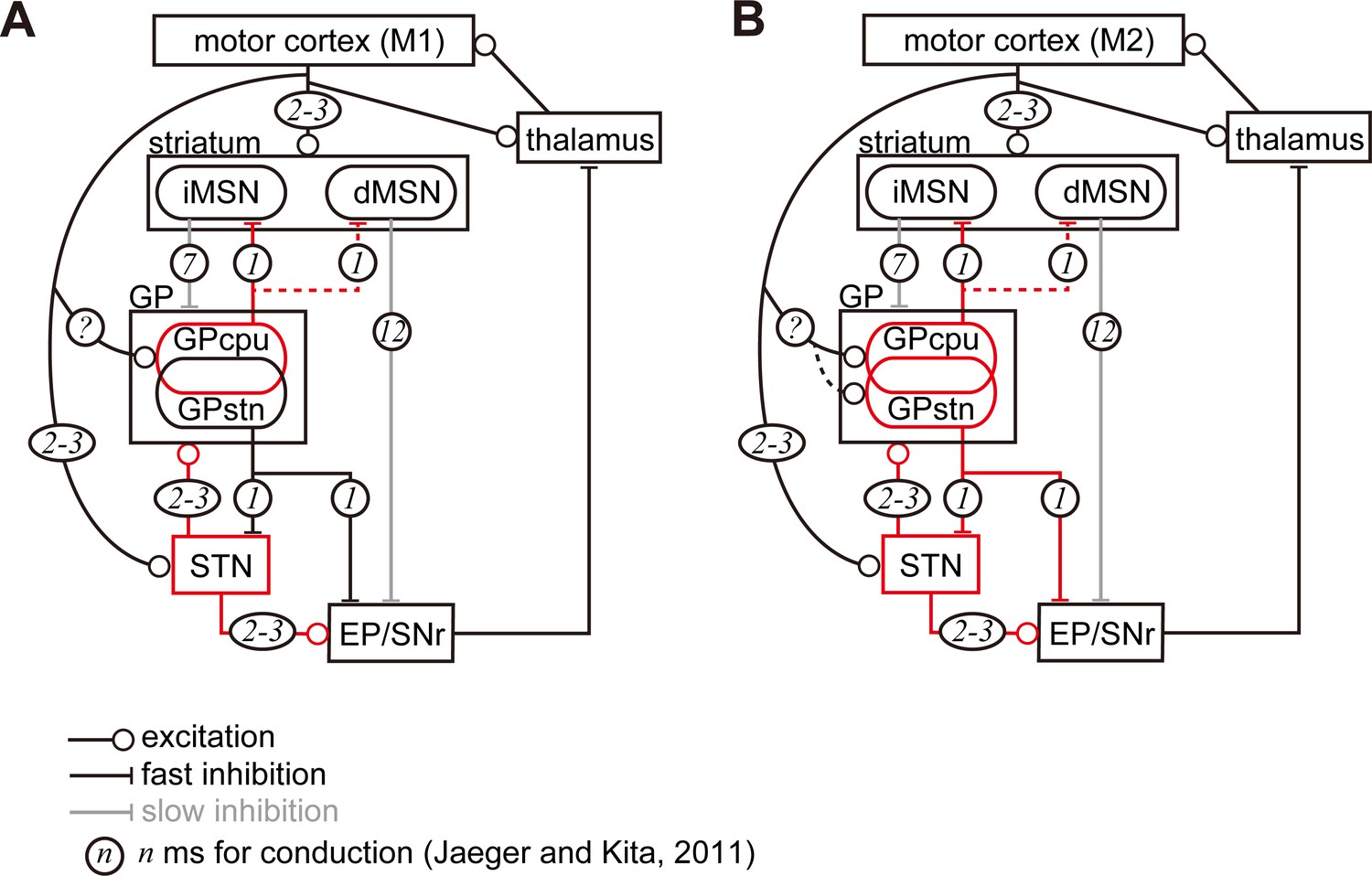
Diagram of cortico-basal ganglia-thalamus circuitry.
The dotted lines represent the relatively weak innervation reported in this study for cortex to GPSTN, and for GPCPu to dMSNs (Glajch et al., 2016). The numbers in circles indicate estimated conduction times in milliseconds (ms) (Jaeger and Kita, 2011). (A) M1 activation induces excitation in the striatum, STN, and GPCPu. Due to the electrophysiological properties of the neurons, STN and GP may be activated faster than striatal neurons. (B) M2 activation conveys additional excitation to the GPSTN neurons. The possible information flow related to the present study is indicated by red lines. Note that inhibition from the GP is here considered faster (1 ms) than excitation from the STN (2–3 ms) (Jaeger and Kita, 2011). The actual timing of spike activity depends on neuron type, and excitation/inhibition interactions are complex.
Tables
Table 1
Electrophysiological properties of globus pallidus (GP) neurons.
https://doi.org/10.7554/eLife.49511.012| GPSTN (N = 108) | GPCPu (N = 65) | p-value | |
|---|---|---|---|
| Mean membrane potential (mV) | −46.63 ± 4.95 (−34.2– −61.53) | −46.36 ± 5.9 (−33.59– −60.53) | 0.682 |
| Input resistance (MΩ) | 232.35 ± 131.87 (33.1–887.45) | 329.97 ± 168.19 (32.8–828.3) | 6.8 × 10−05 *** |
| Time constant (ms) | 12.94 ± 10.23 (2.25–79.75) | 21.92 ± 13.11 (2.42–55.67) | 2.1 × 10−07 *** |
| Sag potential (mV) | 7.23 ± 4.52 (1.25–22.02) | 8.71 ± 7 (0.63–35.18) | 0.3432 |
| Spike frequency at 100 pA depolarization (Hz) | 48.46 ± 22.94 (0–103) | 35.81 ± 19.6 (2–85) | 0.00041 *** |
| Spike frequency at 500 pA depolarization (Hz) | 99.14 ± 66.87 (1–244) | 35.24 ± 39.24 (1–172) | 1.8 × 10−09 *** |
| Maximum spike frequency (Hz) | 135.04 ± 65.42 (11–263) | 72.14 ± 36.12 (2–172) | 1.0 × 10−09 *** |
| Current at maximum spike frequency (pA) | 578.63 ± 277.97 (50–1000) | 345.24 ± 219 (50–1000) | 6.9 × 10−08 *** |
| Spike height (mV) | 74.06 ± 9.77 (47.04–96.98) | 76.55 ± 11.69 (38.84–95.97) | 0.051 |
| Spike width (ms) | 0.95 ± 0.29 (0.63–2.29) | 1.19 ± 0.32 0.7–2.17 | 1.6 × 10−09 *** |
| Spike threshold (mV) | −37.57 ± 4.79 (−24.09– −48.11) | −37.7 ± 5.32 (−23.14– −46.03) | 0.5351 |
| fAHP amplitude (mV) | 21.16 ± 5.14 (9.1–38.72) | 18.09 ± 4.57 (11.88–36.34) | 1.3 × 10−05 *** |
| fAHP delay after spike peak (ms) | 0.98 ± 0.39 (0.55–2.7) | 1.31 ± 0.55 (0.6–3.8) | 3.4 × 10−07*** |
| sAHP amplitude (mV) | 18.26 ± 4.2 (9.47–32.87) | 16.54 ± 4.71 (10.38–29.78) | 0.0035 ** |
| sAHP delay after spike peak (ms) | 9.63 ± 3.32 (2.25–16.95) | 22.58 ± 13.54 (2.25–65.5) | 4.5 × 10⁻¹² *** |
| On cell mode spontaneous firing frequency (Hz) | 20.79 ± 18.74 (0–90.53) | 5.47 ± 9.22 (0–35.68) | 1.2 × 10−08 *** |
| Whole cell mode spontaneous firing frequency (Hz) | 19.02 ± 13.74 (0–61.74) | 9.41 ± 9.44 (0–31.85) | 4.0 × 10−06 *** |
-
GPSTN, GP neurons projecting to the subthalamic nucleus; GPCPu, GP neurons projecting to the striatum; fAHP, fast afterhyperpolarization; sAHP, slow afterhyperpolarization; **, p<0.01; ***, p<0.001. Statistical significance was examined using the Wilcoxon rank sum test. The range of each parameter is shown in parentheses.
Table 2
The maximum number of cortical boutons (/100 × 100 μm2) in the basal ganglia nuclei.
https://doi.org/10.7554/eLife.49511.019| Cortical area | GP | Striatum | STN |
|---|---|---|---|
| M1 (N = 4 rats) | 267, 200, 289, 141 | 911, 1300, 1464, 657, | 506, 432, 528, 408 |
| M2 (N = 4 rats) | 317, 737, 513, 92 | 1300, 2021, 1829, 398 | 420, 717, 637, 177 |
Additional files
-
Supplementary file 1
Primary and secondary antibodies used in this study.
- https://doi.org/10.7554/eLife.49511.024
-
Transparent reporting form
- https://doi.org/10.7554/eLife.49511.025
Download links
A two-part list of links to download the article, or parts of the article, in various formats.
Downloads (link to download the article as PDF)
Open citations (links to open the citations from this article in various online reference manager services)
Cite this article (links to download the citations from this article in formats compatible with various reference manager tools)
Motor cortex can directly drive the globus pallidus neurons in a projection neuron type-dependent manner in the rat
eLife 8:e49511.
https://doi.org/10.7554/eLife.49511


