Neural mechanisms of economic choices in mice
- Department of Neuroscience, Washington University, United States
Figures
Figure 1
Economic choices in mice.
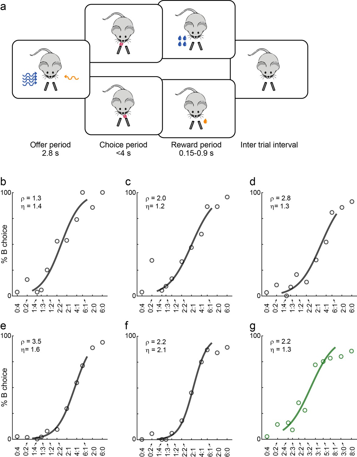
(a) Task diagram. In the experiments, mice chose between two liquid rewards (juices, schematized by the two lick tubes) offered in variable amounts. For each offer, the juice identity (water or sugar water) was represented by the odor identity, and the juice quantity was represented by the odor concentration. (b–f) Choice pattern, example sessions. In each panel, the x-axis represents different offer types in log(qB/qA); the y-axis represents the percent of trials in which the animal chose juice B. Data points are averaged across trials, and the sigmoid is obtained from a logistic regression (Materials and methods, Equation 1). Each panel indicates the relative value (ρ) and the sigmoid steepness (η). The five sessions shown here are from mice M56, M55, M47, M48 and M49, respectively. Forced choices are shown (including error trials) but not included in logistic regressions. (g) Example session of a mouse performing the flipped version of the task (M53).
Figure 2
Behavior, population analysis.
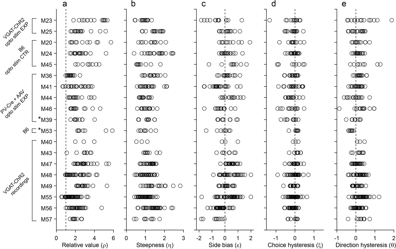
The figure illustrates the entire behavioral data set (19 mice). Each panel illustrates one behavioral measure, each row represents one mouse, and each data point represents one session. Relative value and steepness were obtained from Equation 1; side bias, choice hysteresis and direction hysteresis were obtained from Equations 2-4. Labels on the left indicate for each mouse the strain and the relevant experiment. Asterisks indicate the two mice (M39 and M53) trained in the flipped version of the task. Importantly, the measures obtained for these mice were comparable to those obtained for the other animals. For mice participating in optical inactivation experiments, only trials without stimulation (stimOFF) were included in this figure. (a) Relative value. Averaging across sessions and across animals, we obtained mean(ρ)=2.39 ± 1.01 (mean ± SD). (b) Steepness. Averaging across sessions and across animals, we obtained mean(η)=1.19 ± 0.41 (mean ± SD). (c) Side bias. On any given session, choices could present a side bias, although the direction changed across sessions and across animals. Seven animals presented a consistent bias (p<0.01, t test). Of them, four preferred right and three preferred left, indicating that side biases were not imposed by the experimental apparatus. Averaged across the population, the side bias was rather modest (mean(ε)=0.08 ± 0.04, mean ± SEM). (d) Choice hysteresis. Only one animal presented a consistent effect (p<0.01, t test). Averaged across the population, choice hysteresis was modest (mean(ξ) = –0.08 ± 0.01, mean ± SEM). (e) Direction hysteresis. Six animals presented a consistent effect (p<0.01, t test). For one of them the effect was negative. Averaged across the population, direction hysteresis was significant but fairly modest (θ = 0.15 ± 0.02, mean ± SEM).
Figure 3

LO inactivation disrupts economic decisions, example sessions.
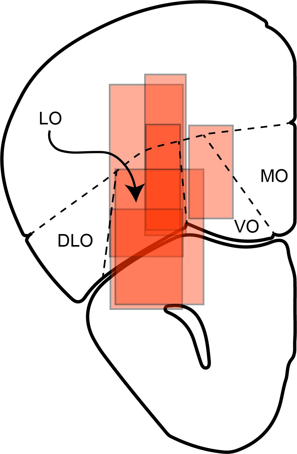
(a) Effect of LO inactivation measured in a VGAT-ChR2 mouse. (b–f) Effect measured in PV-Cre+AAV-DIO-ChR2 mice. Each panel illustrates one session. Red data points represent trials in which area LO was inactivated through optical stimulation of GABAergic interneurons (stimulation ON). Black data points represent normal conditions (stimulation OFF). Each panel indicates the relative value (ρ) and the sigmoid steepness (η) measured in each condition. As a result of LO inactivation, ρ varied in a seemingly erratic way, while η consistently increased (shallower sigmoids). The six sessions shown here are from mice M25, M24, M36, M46, M41 and M41, respectively. (g) Histological analysis of adeno-associated virus (AAV) injections. The infected area for five mice are overlaid in gray scale (mouse atlas, sections A2.68 and A2.22) (Franklin and Paxinos, 2013). Red triangles indicate the locations of the optical fiber tips.
Figure 4
Effects of LO inactivation, relative value.
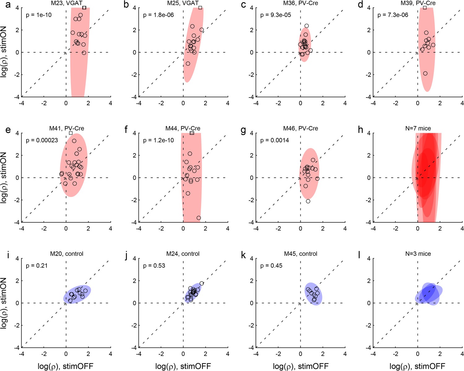
(a, b) Results for two VGAT-ChR2 mice. Each panel illustrates the results for one animal. The x- and y-axes represent the log relative value, log(ρ), measured under normal conditions (stimOFF) and under LO inactivation (stimON), respectively. Each data point represents one session. Outliers are clipped to the axes and indicated with a square. Shaded ellipses represent the 90% confidence interval for the corresponding distribution. Under normal conditions, log(ρ)>0 and the distribution across sessions was relatively narrow in both animals. As a result of LO inactivation, log(ρ) increased or decreased, in way that appeared erratic. The resulting distribution for log(ρ) was much wider (ellipses are elongated along the vertical axis). This effect was highly significant in both animals. The p value indicated in each panel is from an F test for equality of variance. (c–g) Results for five PV-Cre + AAV-DIO-ChR2 mice. The results closely resemble those in panels (ab). (h) Combined results for seven experimental mice. The ellipses illustrated in panels (a–g) are superimposed here. (i–k) Results for three control mice (see Results). Same convention as in (a). In this case, the log(ρ) measured under optical stimulation was generally indistinguishable from that measured under normal conditions. (l) Combined results for three control mice.
Figure 5
Effects of LO inactivation, sigmoid steepness.
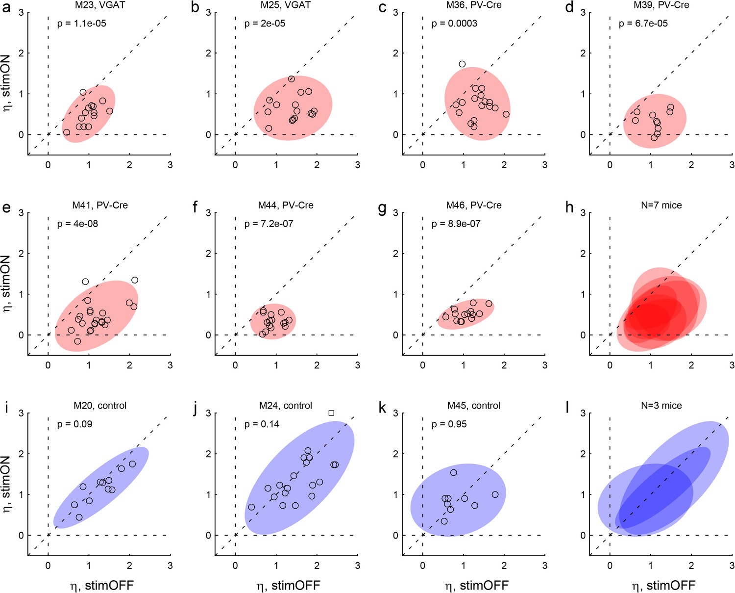
(a, b) Results for two VGAT-ChR2 mice. The x- and y-axes represent the sigmoid steepness (η) measured under normal conditions (stimOFF) and under LO inactivation (stimON), respectively. Each data point represents one session and shaded ellipses represent the 90% confidence interval for the corresponding distribution. Under normal conditions, η varied somewhat from session to session. Independently of the measure obtained under normal conditions, LO inactivation consistently reduced the sigmoid steepness (data points lie below the identity line). In other words, LO inactivation increased choice variability (choices became more noisy). This effect was highly significant in both animals. The p value indicated in each panel is from a paired t test. (c–g) Results for five PV-Cre + AAV-DIO-ChR2 mice. The results closely resemble those in panels (ab). (h) Combined results for seven experimental mice. (i–k) Results for three control mice. For these animals, the steepness measured under optical stimulation was generally indistinguishable from that measured under normal conditions (data points lie on the identity line). (l) Combined results for three control mice.
Figure 6 with 3 supplements
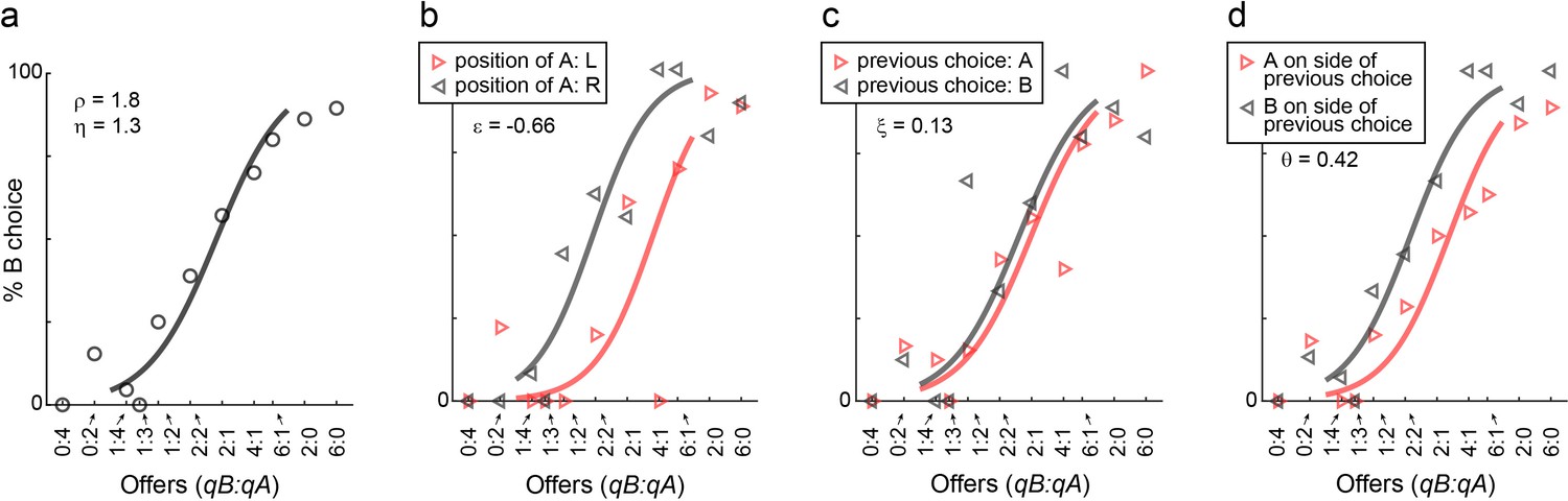
Choice biases, example session.
(a) Example session (M57), same format as in Figure 1. (b–d) Choice biases. For the session in panel (a), the three panels illustrate the side bias (b), the choice hysteresis (c) and the direction hysteresis (d). In (b), trials were divided depending on the position of juice A (left or right). In (c), trials were divided depending on the juice chosen on the previous trial (A or B). In (d), trials were divided depending on whether juice A was offered on the side chosen in the previous trial or on the other side. In each panel, data points are averages across trials. Sigmoids were obtained from logistic regressions (Materials and methods, Equations 2-4) and each panel indicates the corresponding parameter (ε, ξ, θ).
Figure 6—figure supplement 1
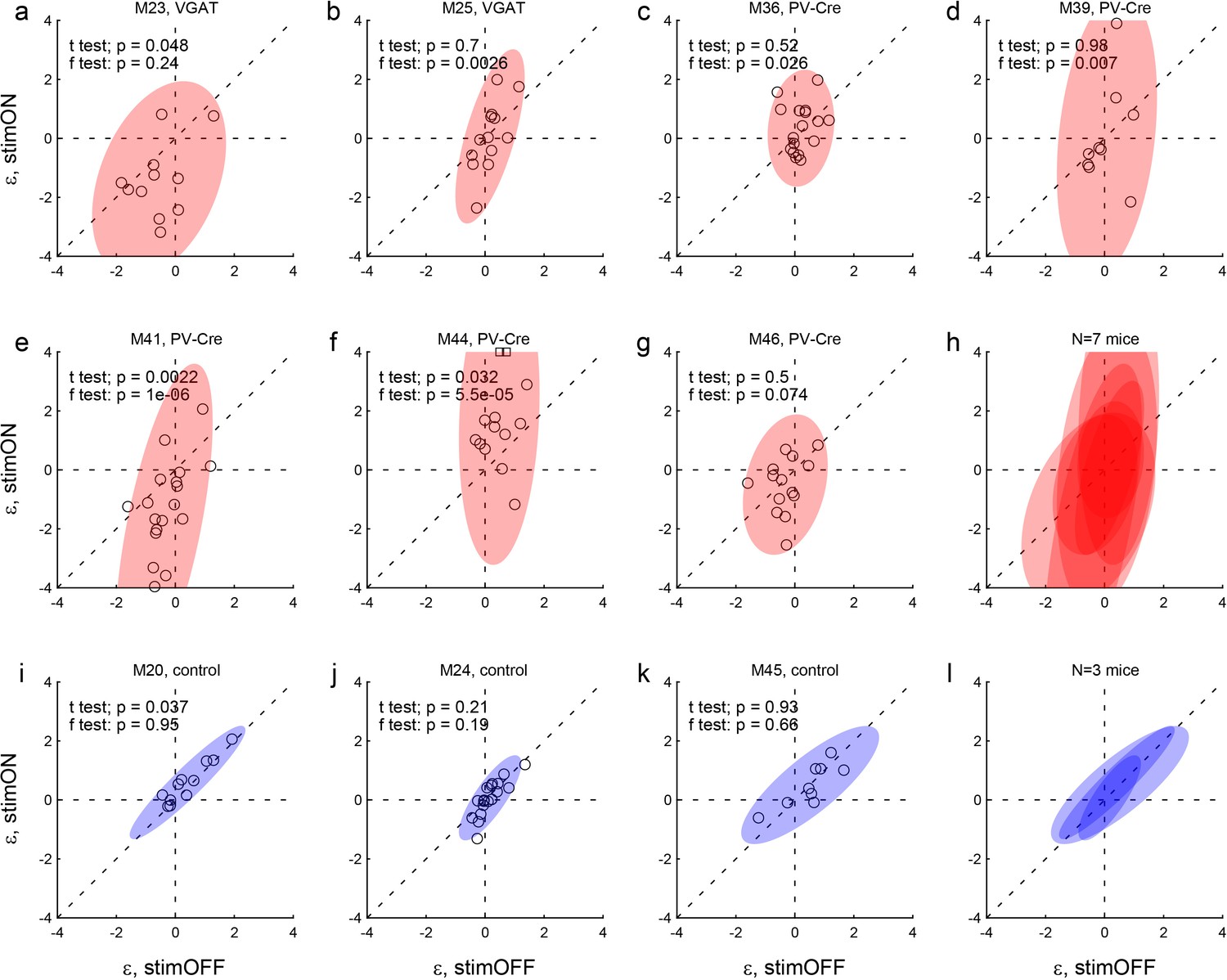
Effects of LO inactivation, side bias.
Same format as in Figure 4. (a–h) Results for two VGAT-ChR2 mice (a,b) and five PV-Cre + AAV-DIO-ChR2 mice (c–g). The x- and y-axes represent the side bias (ε) measured under normal conditions (stimOFF) and under LO inactivation (stimON), respectively. Each data point represents one session and shaded ellipses represent the 90% confidence interval for the corresponding distribution. For most mice, the distribution under LO inactivation is elongated on the y-axis – an effect quantified by the F test (see p value in each panel). In other words, LO inactivation induced systematic side biases. Interestingly, side biases were not stereotyped across sessions – any one animal presented a left (ε <0) or right (ε >0) bias in different sessions. (i–l) Results for control mice.
Figure 6—figure supplement 2
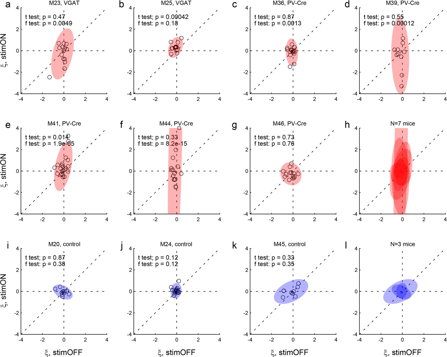
Effects of LO inactivation, choice hysteresis.
Same format as in Figure 4. (a–h) Results for two VGAT-ChR2 mice (a,b) and five PV-Cre + AAV-DIO-ChR2 mice (c–g). For most mice, the distribution under LO inactivation is elongated on the y-axis – an effect quantified by the F test (p value indicated in each panel). In other words, in many sessions, LO inactivation induced a systematic bias. Note that in some cases LO inactivation resulted in a negative choice hysteresis (ξ <0), equivalent to a tendency to alternate choices between juices. (i–l) Results for control mice.
Figure 6—figure supplement 3

Effects of LO inactivation, direction hysteresis.
Same format as in Figure 4. (a–h) Results for two VGAT-ChR2 mice (a,b) and five PV-Cre + AAV-DIO-ChR2 mice (c–g). For most mice, the distribution under LO inactivation is elongated on the y-axis – an effect quantified by the F test (p value indicated in each panel). Thus LO inactivation often induced a systematic bias. In some cases, LO inactivation resulted in a negative direction hysteresis (θ <0), equivalent to a tendency to alternate choices between sides. (i–l) Results for control mice.
Figure 7
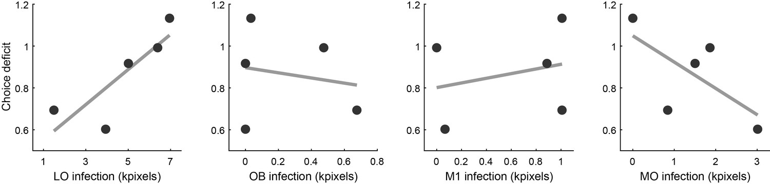
Relation between choice deficit and infection in four brain areas.
Panels from left to right illustrate the results obtained for area LO, the olfactory bulb (OB), primary motor cortex (M1) and the medial orbital area (MO). In each panel, the x-axis represents the infection size (i.e., a proxy for the level of inactivation under optical stimulation). The y-axis represents the choice deficit, with higher values corresponding to more severe impairments. Each data point represents one animal. Only for area LO did infection size and choice deficit correlate in the predicted direction. For OB and M1 there was no correlation. For MO, the correlation was in the opposite direction.
Figure 8
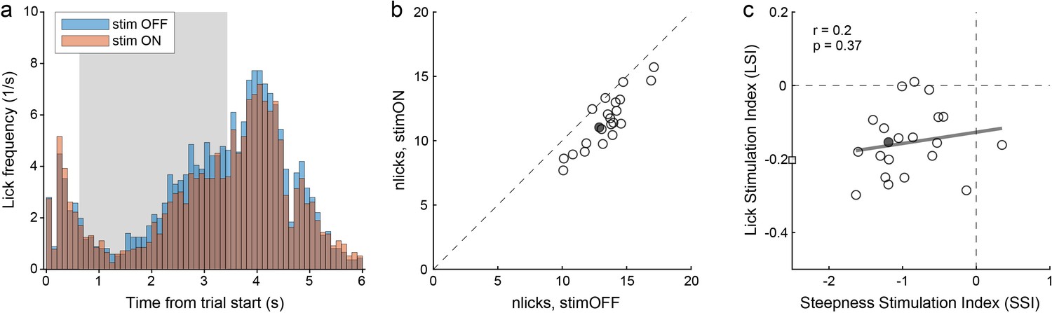
Choice deficits were not caused by motor impairments.
(a) Licking activity in one representative session (from mouse M41). The plot illustrates the licking frequency (y-axis) over the course of the trial under normal conditions (stim OFF) and under optical stimulation (stim ON). The gray shade highlights the stimulation period. All trials were included in the figure. Notably, the licking frequency decreased somewhat under stimulation. Indeed, for this session we measured LSI = –0.15. (b) Effects of optical stimulation on licking across sessions (mouse M41). The axes represent the average number of licks measured in stim OFF trials (x-axis) and in stim ON trials (y-axis). Measures were obtained from the time window 1.5–4.5 s after the trial start. Each data point represents one session, and the filled data point indicates the session in panel (a). Stimulation reduced licking consistently but modestly. For this animal, we measured mean(LSI) = –0.16. (c) Relation between choice deficits and motor effects (mouse M41). The axes represent the primary effect of optical stimulation on choice (SSI, x-axis) and that on licking (LSI, y-axis). Each data point represents one session, the filled data point represents the session in panel (a), and the square represents an outlier. The gray line was obtained from a linear regression (excluding the outlier). LSI and SSI were not correlated across sessions (r = 0.2, p=0.37). Similarly, we did not find any correlation between LSI and SSI in any of the other 4 PV-Cre mice (all r < 0.2, all p>0.35).
Figure 9

Encoding of decision variables, example neurons.
(a) Response encoding the offer value left (from left hemisphere, post-offer time window). In the left panel, firing rates are plotted against the offer type, and black dots show the behavior. Diamonds and circles indicate trials in which the animal chose juice A and juice B, respectively. Red and blue symbols indicate trials in which the animal chose the offer on the left and right, respectively. Thus red diamonds and blue circles correspond to trials in which juice A was offered on the left; red circles and blue diamonds correspond to trials in which juice A was offered on the right. Error bars indicate SEM. The cell activity increased as a function of the value offered on the left, independently of the juice type and the animal's choice. This point is most clear in the right panel, where the same neuronal response is plotted against the variable offer value left (expressed in units of juice B). The black line is from a linear regression, and the R2 is indicated in the figure. (b) Response encoding the offer value right (right hemisphere, late delay). This neuron was recorded in the right hemisphere. (c) Response encoding the chosen side (right hemisphere, late delay). In this case, the cell activity was nearly binary. It was high when the animal chose the offer on the right (blue) and low when the animal chose the offer on the left (red), irrespective of the chosen juice (diamonds for A, circles for B). (d) Response encoding the chosen side (right hemisphere, post-juice). (e) Response encoding the chosen value (right hemisphere, late delay). This response increased as a function of the value chosen by the animal, independent of the juice type and the spatial contingencies. (f) Response encoding the position of A (left hemisphere, late delay). The cell activity was nearly binary. It was high when juices A and B were respectively offered on the left and on the right; it was low when the spatial contingencies were reversed. Note that the two outliers data points corresponds to forced choices, where juice B was not offered. Conventions in panels b-f are as in panel a.
Figure 10
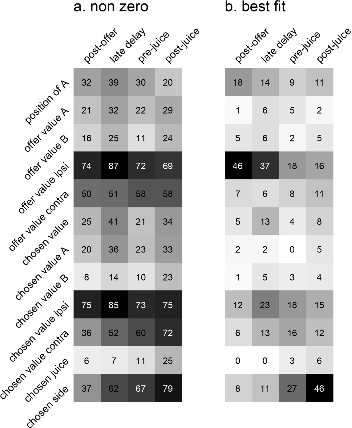
Encoding of decision variables, population analysis.
(a) Explained responses. This panel shows, for each variable and for each time window, the number of responses explained. For example, 32 responses in the post-offer time window were explained by the variable position of A. Because each response could be explained by more than one variable, each response may contribute to multiple bins in this plot. Gray shades recapitulate the cell counts. (b) Best fit. Each response was assigned to the variable that provided the highest R2, and the number of responses obtained are shown here. In this panel, each response contributes to (at most) one bin. Notably, many responses were best explained by variables offer value ipsi and chosen side.
Figure 11
Variable selection analysis.
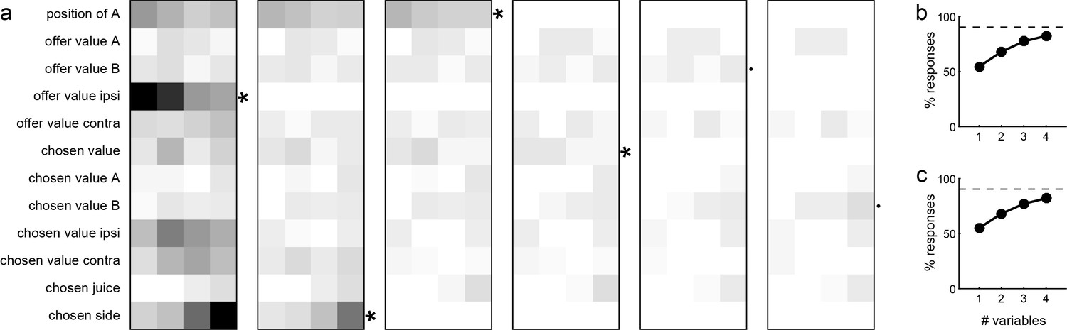
(a) Stepwise selection. The leftmost panel is as in Figure 10b. At each iteration, we identified the bin with the highest number of responses and we selected the corresponding variable. If the marginal explanatory power was ≥5%, we retained the variable and removed from the pool all the responses explained by that variable. At each iteration, we also verified that the marginal explanatory power of variables selected in previous iterations remained ≥5% once the new variable was selected. In the first four iterations, the procedure selected variables offer value ipsi, chosen side, position of A and chosen value. Variables selected in subsequent iterations failed the 5% criterion and were thus rejected. (b) Percent of explained responses, stepwise procedure. The plot illustrates the percent of responses explained (y-axis) as a function of the number of variables (x-axis). On the y-axis, 100% corresponds to the number of responses passing the ANOVA criterion in one of the four time windows (n = 555); the dotted line corresponds to the number of responses collectively explained by the 12 variables included in the analysis (n = 501). The four selected variables explained 457 responses, corresponding to 91% of the responses explained by all 12 variables. (c) Best-subset procedure. The plot illustrates the percent of responses explained (y-axis) as a function of the number of variables (x-axis).
Figure 12
Reconstructed locations of neuronal recordings for six mice.
Recording regions for all animals were transferred on the same hemisphere. Approximate AP coordinate of this section is bregma 2.68 mm, interaural 6.48 mm.
Tables
Table 1
Results of ANOVAs.
The table reports the results of two ANOVAs. Each column represents one factor, each row represents one time window, and numbers represent the number of cells significantly modulated by the corresponding factor (p<0.001). The bottom row indicates the number of cells that pass the criterion in at least one of the five time windows. The three left-most columns report the results of a 3-way ANOVA. Notably, many cells were modulated by each of the three factors. The right-most column reports the results of a 1-way ANOVA (factor trial type). In total, 301/717 (42%) cells passed the p<0.001 criterion in at least one time window. Neuronal responses that passed this test (N = 565) were identified as task-related and included in subsequent analyses.
| 3-way | 1-way | |||
|---|---|---|---|---|
| Offer type | Position of A | Chosen side | Trial type | |
| Pre-offer | 1 | 4 | 6 | 8 |
| Post-offer | 55 | 35 | 102 | 121 |
| Late delay | 87 | 40 | 123 | 158 |
| Pre-juice | 39 | 27 | 127 | 121 |
| Post-juice | 58 | 28 | 150 | 155 |
| At least 1 | 154 | 85 | 308 | 301 |
Table 2
Variables defined in the analysis of neuronal responses.
| Variable | Definition | |
|---|---|---|
| 1 | position of A | Binary; one if juices A/B are offered on ipsi/contra sides, 0 otherwise |
| 2 | offer value A | Value of juice A offered |
| 3 | offer value B | Value of juice B offered |
| 4 | offer value ipsi | Value offered on the ipsi-lateral side |
| 5 | offer value contra | Value offered on the contra-lateral side |
| 6 | chosen value | Value of the chosen juice |
| 7 | chosen value A | Chosen value if juice A chosen, 0 otherwise |
| 8 | chosen value B | Chosen value if juice B chosen, 0 otherwise |
| 9 | chosen value ipsi | Chosen value if ipsi side is chosen, 0 otherwise |
| 10 | chosen value contra | Chosen value if contra side is chosen, 0 otherwise |
| 11 | chosen juice | Binary; one if juice A is chosen, 0 if juice B is chosen |
| 12 | chosen side | Binary; one if ipsi side is chosen, 0 if contra side is chosen |
Additional files
Download links
A two-part list of links to download the article, or parts of the article, in various formats.
Downloads (link to download the article as PDF)
Open citations (links to open the citations from this article in various online reference manager services)
Cite this article (links to download the citations from this article in formats compatible with various reference manager tools)
Neural mechanisms of economic choices in mice
eLife 9:e49669.
https://doi.org/10.7554/eLife.49669


