Figures and data in A mechanism for hunchback promoters to readout morphogenetic positional information in less than a minute

Figures
Tables
Additional files

19 figures, 1 table and 2 additional files

Figures

Figure 1

Download asset Open asset

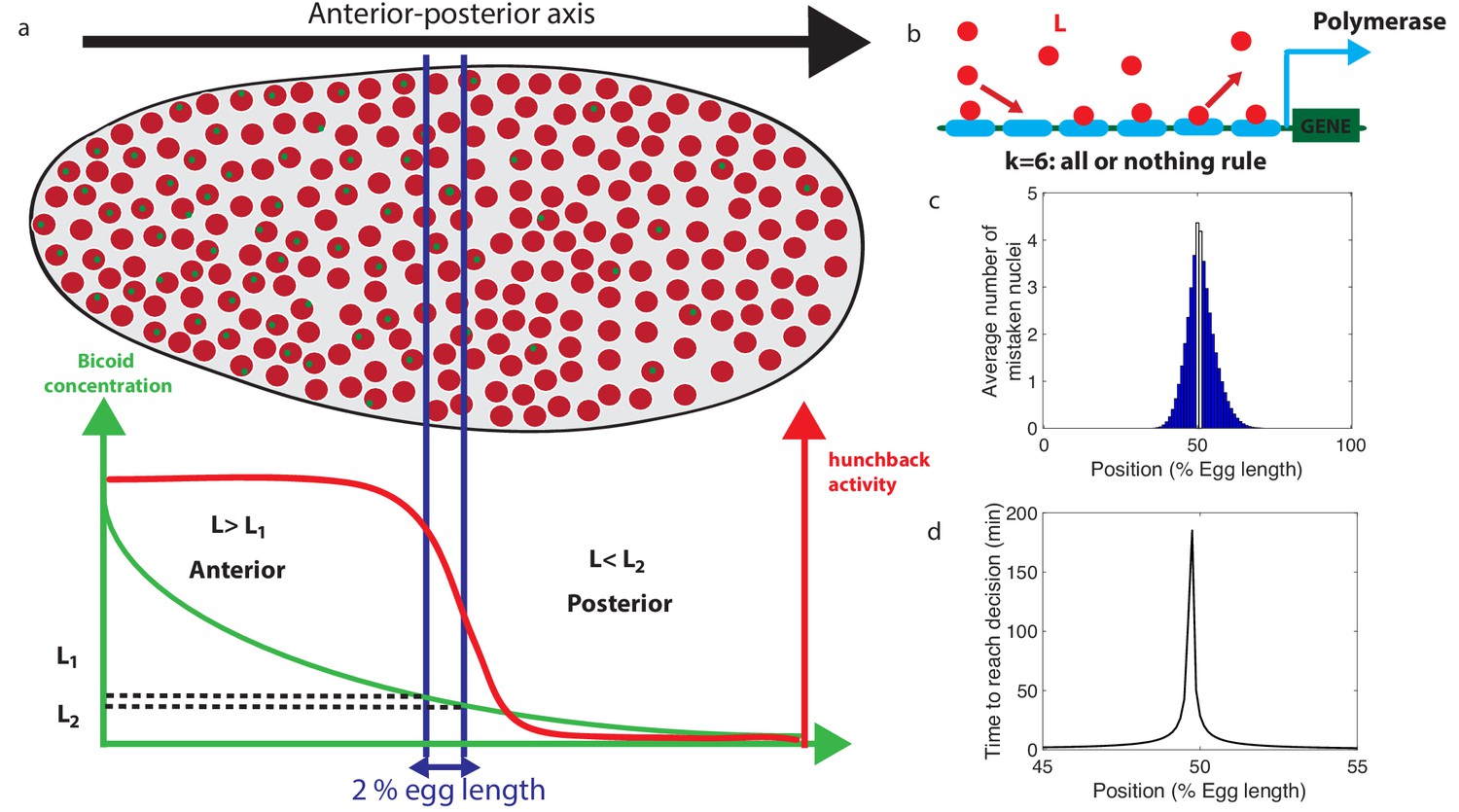
Decision between anterior and posterior developmental blueprints.

(a) The early *Drosophila* embryo and the Bicoid morphogen gradient. The cartoon shows a projection on one plane of the embryo at nuclear cycles 10–13, when nuclei (red dots) have migrated to the surface of the embryo (O'Farrell, 2015). The activity of the *hunchback* gene decreases along the Anterior-Posterior (AP) axis. The green dots represent active transcription loci. The average concentration L(x) of maternal Bicoid decreases exponentially along the AP axis by about a factor five from the anterior (left) to the posterior (right) ends. Between the blue lines lies the boundary region. Its width δ_x is 2% of the egg length. *hunchback* activity decreases along the AP axis and undergoes a sharp drop around the boundary region. The half-maximum Bcd concentration position in WT embryos is shifted by about 5% of the egg-length toward the anterior with respect to the mid-embryo position (Struhl et al., 1992). We consider this *hunchback* half maximum expression as a reference point when describing the AP axis of the embryo. The *hunchback* readout defines the cell fate decision whether each nucleus will follow an anterior or the posterior gene expression program. (b) A typical promoter structure contains six binding sites for Bicoid molecules present at concentration L. $k = 6$ indicates that the gene is active only when all binding sites are occupied, defining an all-or-nothing promoter architecture. Other forms and details of the promoter structure will be discussed in Figure 2 and Figure 3. (c) The average number of nuclei making a mistake in the decision process as a function of the egg length position at cycle 11. For a fixed-time decision process completed within $T = 270$ seconds (and $k = 6$ , that is, all-or-nothing activation scheme), a large number of nuclei make the wrong decision (full blue bars). $T = 270$ seconds is the duration of the interphase of nuclear cycle 11 (Tran et al., 2018). For nuclei located in the boundary region either answer is correct so that we leave these bars unfilled. Most errors happen close to the boundary, as intuitively expected. See Appendix 1 for a detailed description of how the error is computed for the fixed-time decision strategy. (d) The time needed to reach the standard error probability of 32% (Gregor et al., 2007a) for the same process as in panel c (see also the subsection 'How many nuclei make a mistake?’) as a function of egg length position. Decisions are easy away from the center but the time required for an accurate decision soars close to the boundary up to 50 min – much longer than the embryological times. Parameters for panels (c) and (d) are six binding sites that bind and unbind Bicoid without cooperaivity and a diffusion limited on rate per site $μ_{max} L = 0.124 s^{- 1}$ , and an unbinding rate per site $ν_{1} = 0.0154 s^{- 1}$ that lead to half activation in the boundary region.

Figure 2

Download asset Open asset

The relation between promoter structure and on-the-fly decision-making.

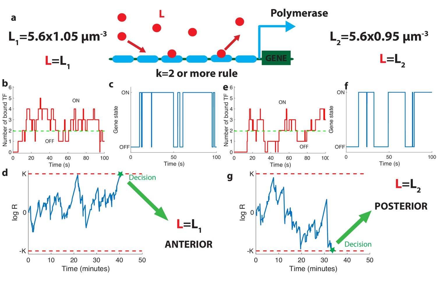
(a). Using six Bicoid binding sites, the promoter decides between two hypothetical Bcd concentrations $L = L_{1}$ and $L = L_{2}$ , given the actual (unknown) concentration L in the nucleus. The number of occupied Bicoid sites fluctuates with time (b) and we assume the gene is expressed (c) when the number of occupied Bicoid binding sites on the promoter is $\geq k$ (green dashed line, here $k = 2$ ). The gene activity defines a non-Markovian telegraph process. The ratio of the likelihoods that the time trace of this telegraph process is generated by $L = L_{1}$ vs $L = L_{2}$ is the log-likelihood ratio used for decision-making (d). The log-likelihood ratio undergoes random excursions until it reaches one of the two decision boundaries (K, −K). In d. the actual concentration is $L = L_{1}$ and the log-likelihood ratio hits the upper barrier and makes the right decision. When $L = L_{2}$ , less Bicoid-binding sites are occupied (e) and the gene is less likely to be expressed (f), resulting in a negative drift in the log-likelihood ratio, which directs the random walk to the lower boundary −K and the $L = L_{2}$ decision (g). We consider that all six binding sites bind Bicoid independently and are identical with binding rate per site $μ_{max} L = 0.07 s^{- 1}$ and unbinding rate per site $ν_{1} = 0.08 s^{- 1}$ , $e = 0.2$ , $k = 2$ , $L = L_{1} = 5.88 μ m^{- 3}$ for panels (b, c, d) and $L = L_{2} = 5.32 μ m^{- 3}$ (e, f, g).

Figure 3

Download asset Open asset

Comparing the performance of two promoter activation rules.

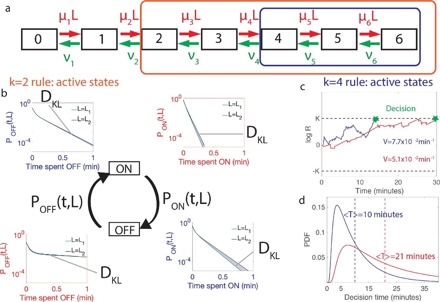
(a) The dynamics of the six Bcd binding site promoter is represented by a seven state Markov chain where the state number indicates the number of occupied Bicoid-binding sites. The boxes indicate the states in which the gene is expressed for the 2-or-more activation rule (red box and red in panels **b-d**) where the gene is active when 2-or-more TF are bound and the 4-or-more activation rule (blue box and blue in panels **b-d**) where the gene is active when 4-or-more TF are bound. (b) The dynamics of TF binding translates into bursting and inactive periods of gene activity. The OFF and ON time distributions are different for the two hypothetical concentrations (blue boxes for $k = 4$ and red boxes for $k = 2$ ). The Kullback-Leibler divergence between the distributions for the two hypothetical concentrations ( $D_{K L}$ ) sets the decision time and is related to the difference in the area below the two distributions. For the $k = 4$ activation rule, the OFF time distributions are similar for the two hypothetical concentrations but the ON times distributions are very different. The ON times are more informative for the $k = 4$ activation rule than the $k = 2$ activation rule (c) The drift V of the log-likelihood ratio characterizes the deterministic bias in the decision process. The differences in (b) translate into larger drift for $k = 4$ for the same binding/unbinding dynamics. (d) The distribution of decision times (calculated as the first-passage time of the log-likelihood random walk) decays exponentially for long times. Higher drift leads to on average faster decisions than for the $k = 4$ activation rule (mean decision times are shown in dashed lines). For all panels the six binding sites are independent and identical with $L = L_{1} = 5.88 μ m^{- 3}$ , $L_{2} = 5.32 μ m^{- 3}$ , $e = 0.1$ , $μ_{max} L = 0.14 s^{- 1}$ and $ν = 0.08 s^{- 1}$ for all binding sites.

Figure 4

Download asset Open asset

Performance, constraints and statistics of fastest decision-making architectures.

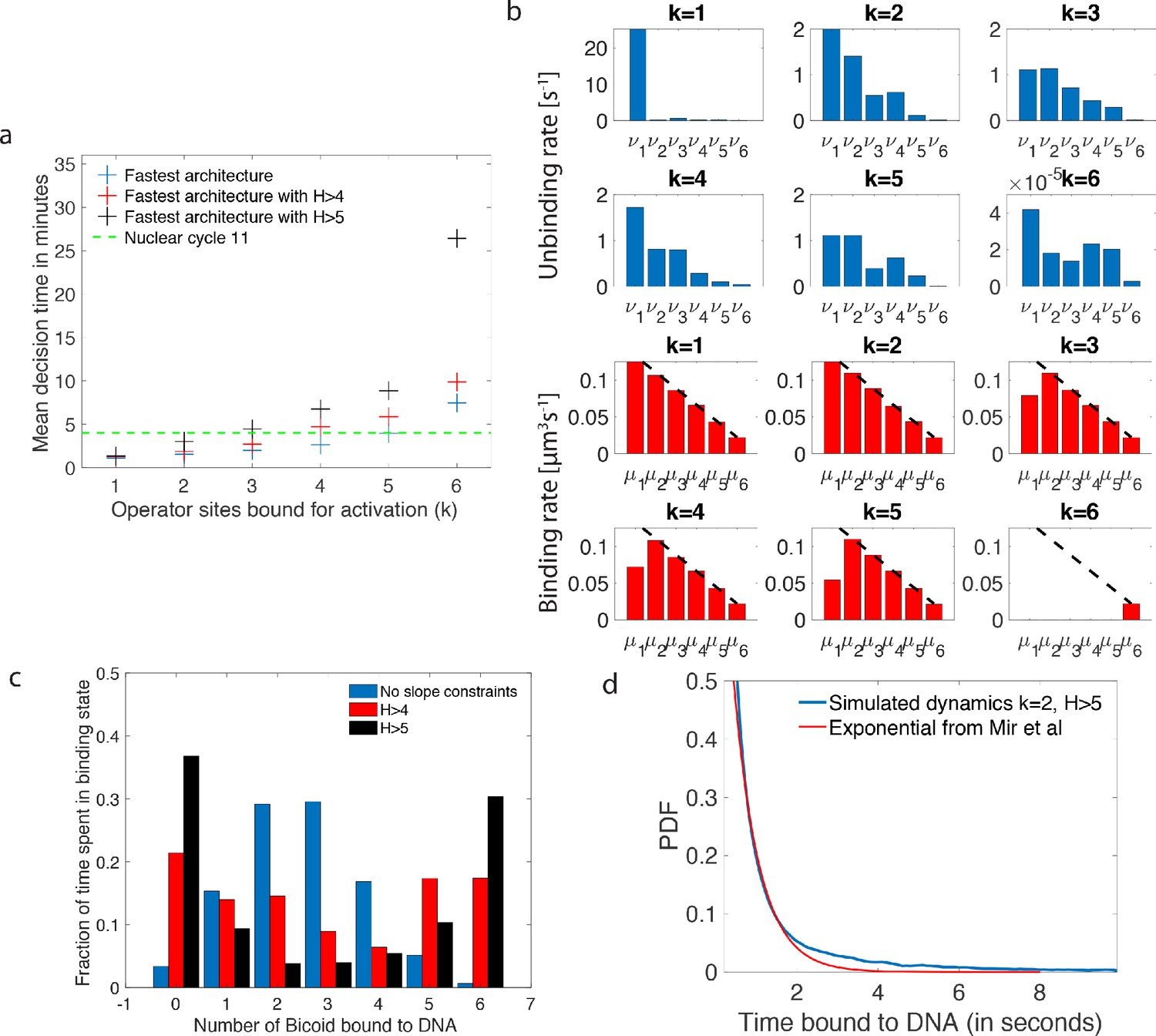
(a) Mean decision time for discriminating between two concentrations with $| L_{2} - L_{1} | = 0.1 L$ and $e = 0.32$ . Results shown for the fastest decision-making architectures for different activation rules and steepness constraints. For a given activation rule (k), we optimize over all values of ON rates $μ_{i}$ and OFF rates $ν_{i}$ (see Figure 3a) within the diffusion limit ( $0.124 s^{- 1}$ per site), constraining the steepness H and probability of nuclei to be active at the boundary (see the paragraph ’Additional embryological constraints on promoter architectures’). The green lines denotes the interphase duration of nuclear cycle 11 and even for the strongest constraints ( $H > 5$ ) we identify architectures that make an accurate decision within this time limit. (b) The unbinding rates (blue) and binding rates (red) of the fastest decision-making architectures with $H > 5$ – all these regulatory systems require cooperativity in TF binding to the promoter-binding sites. The dashed line on the ON rates plots shows the upper bound set by the diffusion limit. (c) Histogram of the probability distribution of the time spent in different Bcd-binding site occupancy states for the fastest decision-making architecture for $k = 3$ and no constraints on the slope (blue), $H > 4$ (red) and $H > 5$ (black). (d) Probability distribution of the time spent bound to th DNA by Bicoid molecules for the fastest decision-making architecture with $H > 5$ and $k = 2$ . Our prediction is compared to the exponential distribution with parameters fit by Mir et al., 2017, for the specific binding at the boundary. While the distributions are close, our simulated distribution is not exponential, as expected for the 6-binding site architecture. The non-exponential behavior in the experimental curve is likely masked by the convolution with non-specific binding. We use the boundary region concentration $L = 5.6 μ m^{- 3}$ (see panel b, $k = 2$ for rates).

Figure 5

Download asset Open asset

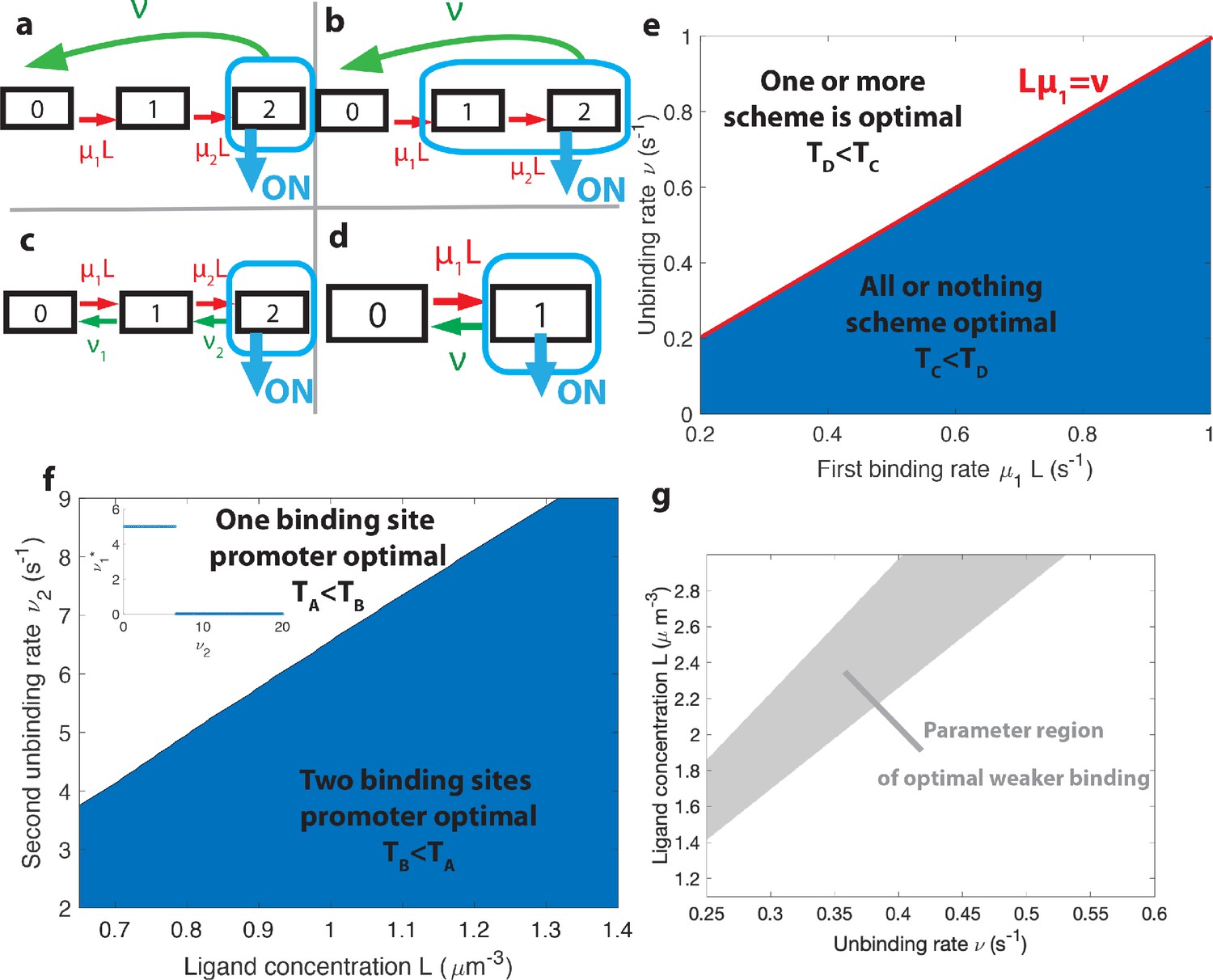
The effects of different promoter architectures on the mean decision time.

We compare promoters of different complexity: the all-or-nothing $k = 2$ out-of-equilibrium model (a), the 1-or-more $k = 1$ out-of-equilibrium model (b), the two binding site all-or-nothing $k = 2$ equilibrium model (c) and the one binding site equilibrium model (d). (e) Comparison of the mean decision time between $k = 2$ (a) and $k = 1$ (b) activation schemes for the two binding site out-of-equilibrium models as a function of the unbinding rate ν and binding rate μ₁. The binding rate μ₂ is fixed to $μ_{2} = μ_{1} / 2$ . The fastest decision-making solution associates the second binding with slower variables to maximize V. Along the line $L μ_{1} = ν$ the activation rules $k = 1$ and $k = 2$ perform at the same speed. $e = 10 %$ . (f) Comparison of the mean decision time for equilibrium architectures with one (d) and two (c) equilibrium TF-binding sites. $μ_{1}, μ_{2}, ν_{1}$ are optimized at fixed $ν_{2}$ , $e = 5 %$ . We set a maximum value of $5 μ m^{3} s^{- 1}$ for μ₁ and μ₂, corresponding to the diffusion limited arrival at the binding site. For ν₁, the maximum value of 5 s⁻¹ corresponds to the inverse minimum time required to read the presence of a ligand, or to differentiate it from unspecific binding of other proteins. Additional binding sites are beneficial at high ligand concentrations and for small unbinding rates. In the blue region, the fastest mean decision time for a fixed accuracy assuming equilibrium binding, comes from a two binding site architecture with a non-zero first unbinding rate. In the white region, one of the binding rates →0 (see inset), which reduces to a one binding site model. $e = 5 %$ . (g) Weaker binding sites can lead to faster decision times within a range of parameters (gray stripe). We consider the $k = 1$ activation scheme with two binding sites (b). For fixed L (x axis), ν (y axis) and $μ_{1} = 0.2 μ m^{3} s^{- 1}$ , we optimize over μ₂ while setting $μ_{2} < μ_{1}$ (context of diffusion limited first and second bindings). The gray regions corresponds to parameters for which the optimal second unbinding rate $μ_{2}^{*} < μ_{1}$ and the second binding is weak. In the white region $μ_{2}^{*} = μ_{1}$ . For all panels $L_{2} = L$ , $L_{1} = 0.95 L$ , $e = 0.05$ .

Figure 6

Download asset Open asset

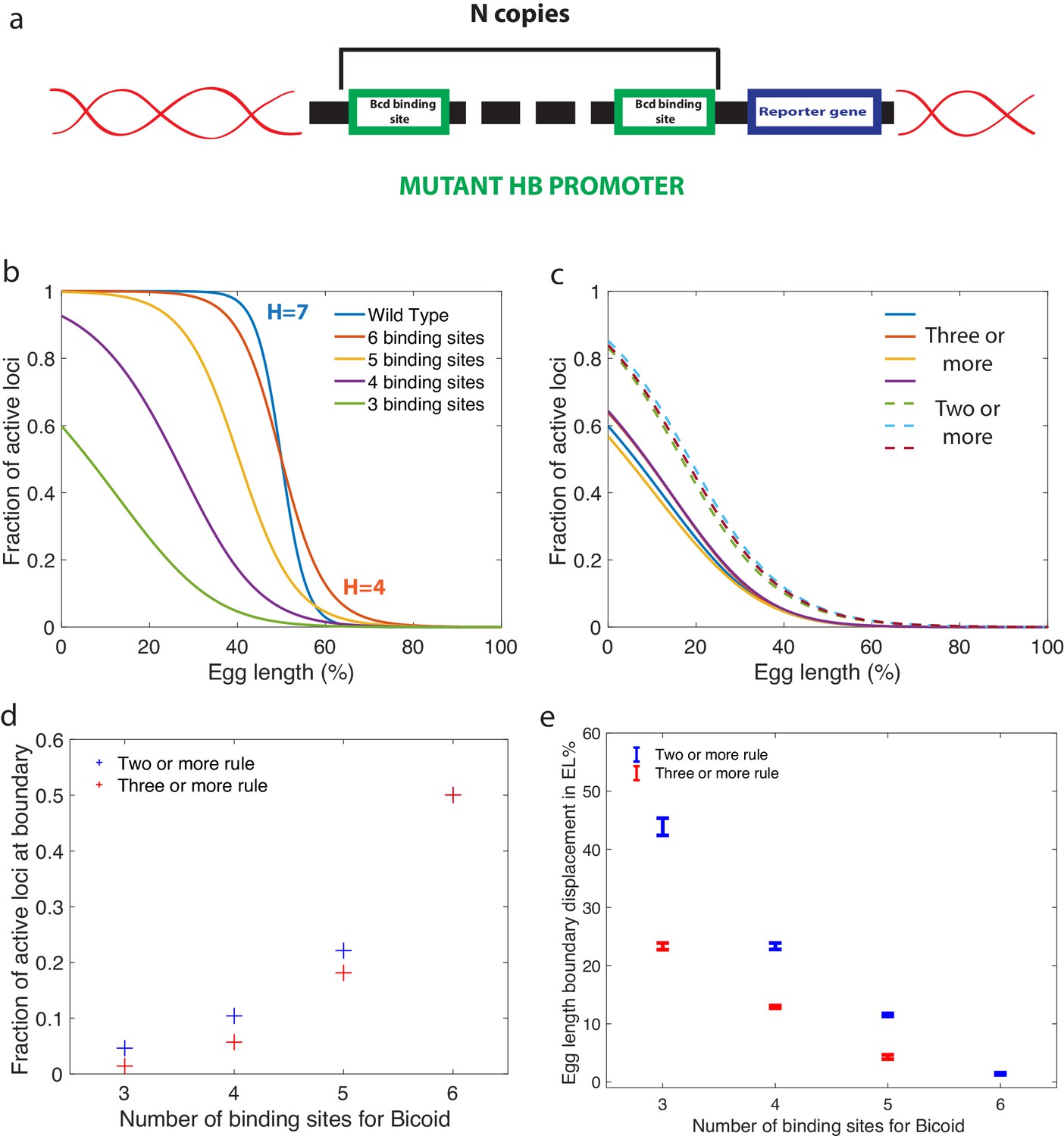
Predictions for experiments with synthetic hb promoters.

(a) We consider experiments involving mutant *Drosophilae* where a copy of a subgroup of the Bicoid-binding sites of the *hunchback* promoter is inserted into the genome along with a reporter gene to measure its activity. (b) The prediction for the activation profile across the embryo for wild type and mutants for the fastest decision time architecture for $H > 4$ and $k = 3$ . (c) The gene activation profile for several architectures for $H > 4$ and $k = 3$ (full lines) and $k = 2$ (dashed lines) that results in mean decision times < 3 minutes. Groups of profiles gather in two distinct clusters. (d) Fraction of genes that are active on average at the $h b$ expression boundary using the minimal $⟨ T ⟩$ architecture identified for $H > 4$ and $k = 3$ as a function of the number of binding sites in the hb promoter. Predictions for the six-binding site cases coincide because having half the nuclei active at the boundary is a requirement in the search for valid architectures. (e) Predicted displacement of the boundary region defined as the site of half *hunchback* expression in terms of egg length as a function of the number of binding sites. The architectures shown result in the fastest decisions for $H > 4$ and $k = 2$ and $k = 3$ . Error bar width is the standard deviation of the various architectures that are close to minimal $⟨ T ⟩$ . For all panels, $L (x)$ has an exponentially decreasing profile with decay length one fifth of total egg length with $L_{0} = 5.6 μ m^{- 3}$ at the boundary. Parameters are given in Appendix 10.

Figure 7

Download asset Open asset

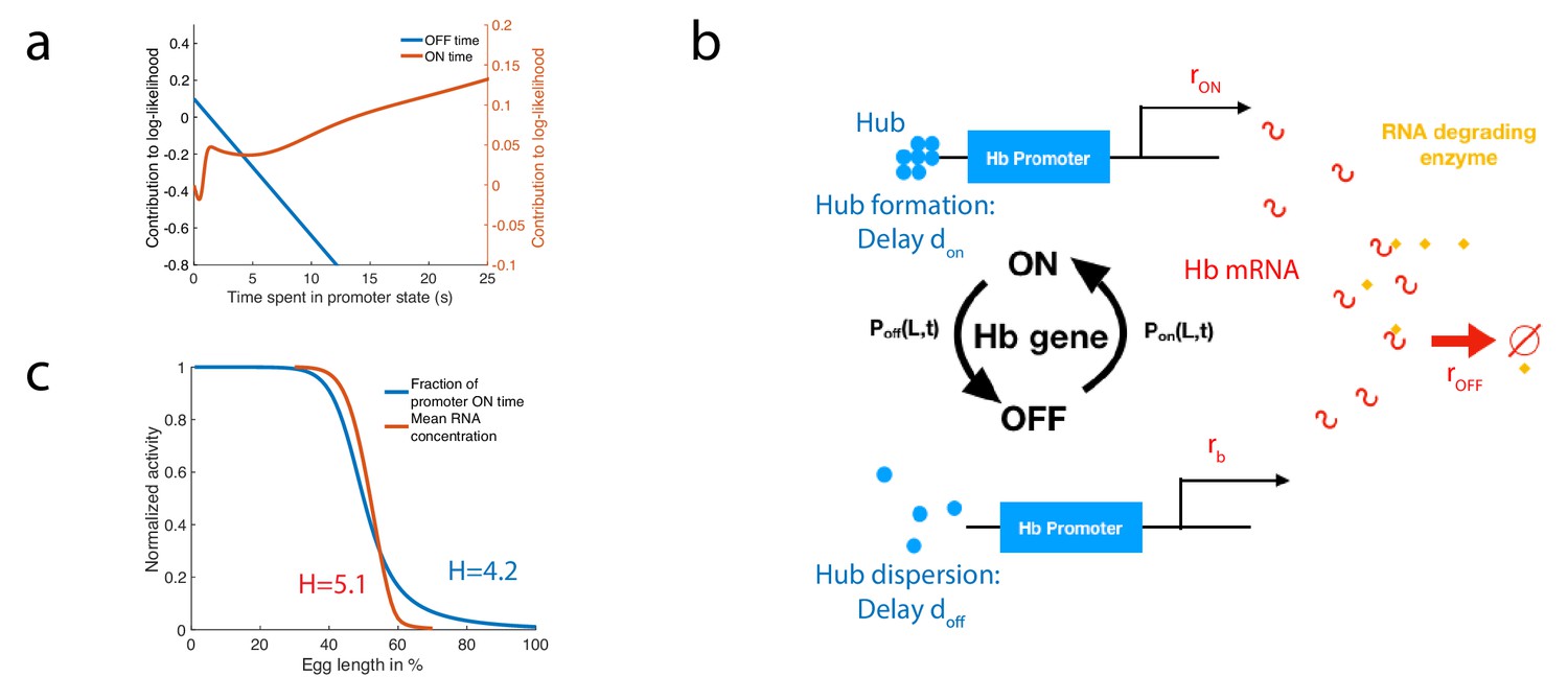
A model of RNA production and degradation approximates the contributions to log-likelihood.

(a) The log-likelihood of different times spent ON (red) and OFF (blue) for the fastest architecture identified with $k = 1$ , $H > 4$ assuming $L = L_{1}$ . The log-likelihood varies linearly with time for long times. (b) The hunchback promoter switches from ON to OFF and from OFF to ON according to the time distributions determined by its gene architecture and activation rule. When ON, after a delay $d_{ON}$ associated with the formation of a cluster or hub (Cho et al., 2016b; Cho et al., 2016a; Mir et al., 2018), RNA is being produced at rate $r_{ON}$ . When OFF, after a delay $d_{O F F}$ , the gene switches to basal rate $r_{b}$ . Hunchback RNA is being degraded actively by an enzyme at rate $r_{OFF}$ . The RNA is in excess for this reaction. (c) The model of RNA production with delay that yields an error of less than 32% in less than 3 min produces a profile of RNA production with high Hill coefficient $≃ 5.2$ (red lines, renormalized RNA profile) that is higher than the Hill coefficient of renormalized gene activity $H ≃ 4$ (blue line). Parameters for promoter activity are those of the fastest architecture identified with $k = 1$ and $H > 4$ , parameters for RNA production are $d_{ON} = 0.047 s$ , $d_{O F F} = 1.6 s$ , $r_{b} = 0.2 s^{- 1}$ s^-1, $r_{OFF} = 0.5 s^{- 1}$ s^-1, $r_{ON} = 0.805 s^{- 1}$ s^-1.

Appendix 2—figure 1

Download asset Open asset

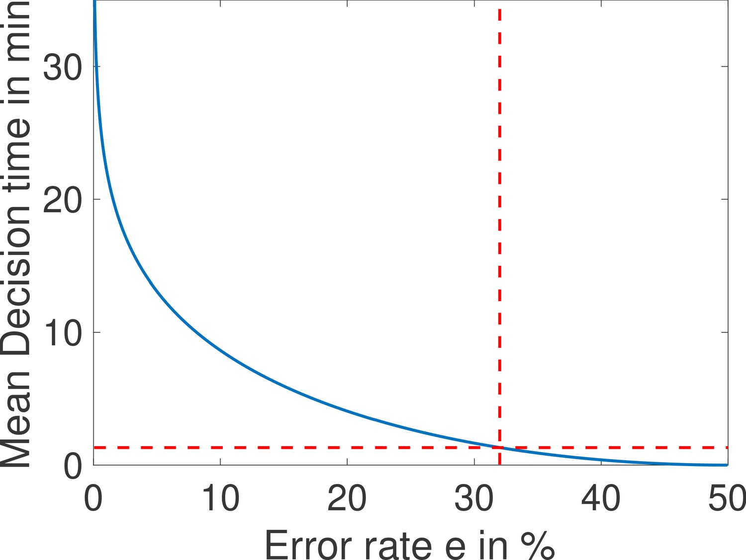
The mean decision time as a function of the error rate e for the fastest architecture identified with $H > 5$ and $k = 1$ (see Main Text Figure 4a).

When the error rate is 32%, decisions are made in less than a minute (red dashed lined). Parameters are $L = L_{1} = 1.05 \cdot 5.6 μ m^{- 3}$ , $L_{2} = 0.95 \cdot 5.6 μ m^{- 3}$ , $μ_{1} = 0.13 μ m^{3} s^{- 1}$ , $μ_{2} = 0.11 μ m^{3} s^{- 1}$ , $μ_{3} = 0.086 μ m^{3} s^{- 1}$ , $μ_{4} = 0.066 μ m^{3} s^{- 1}$ , $μ_{5} = 0.043 μ m^{3} s^{- 1}$ , $μ_{6} = 0.022 μ m^{3} s^{- 1}$ , $ν_{1} = 4.5 s^{- 1}$ , $ν_{2} = 0.042 s^{- 1}$ , $ν_{3} = 0.11 s^{- 1}$ , $ν_{4} = 0.033 s^{- 1}$ , $ν_{1} = 0.037 s^{- 1}$ , $ν_{1} = 0.053 s^{- 1}$ .

Appendix 3—figure 1

Download asset Open asset

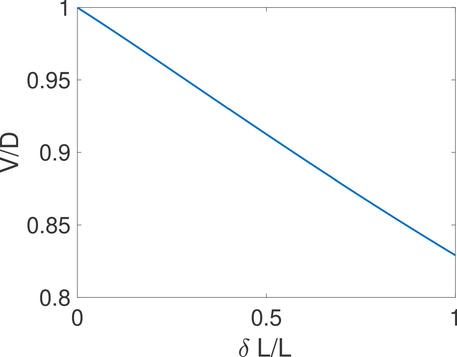
The equality $V = D$ holds for close hypotheses.

We compare the exact drift and diffusion computed from the formulae derived in Siggia and Vergassola, 2013 for the case of one binding site. We find that drift and diffusion are approximately equal for close concentrations (i.e small $δ L / L$ ). Parameters are $ν = 1 s^{- 1}$ , $μ = 1 μ m^{3} s^{- 1}$ , $L_{2} = L = 1 μ m^{- 3}$ , $L_{1} = L + δ L$ .

Appendix 3—figure 2

Download asset Open asset

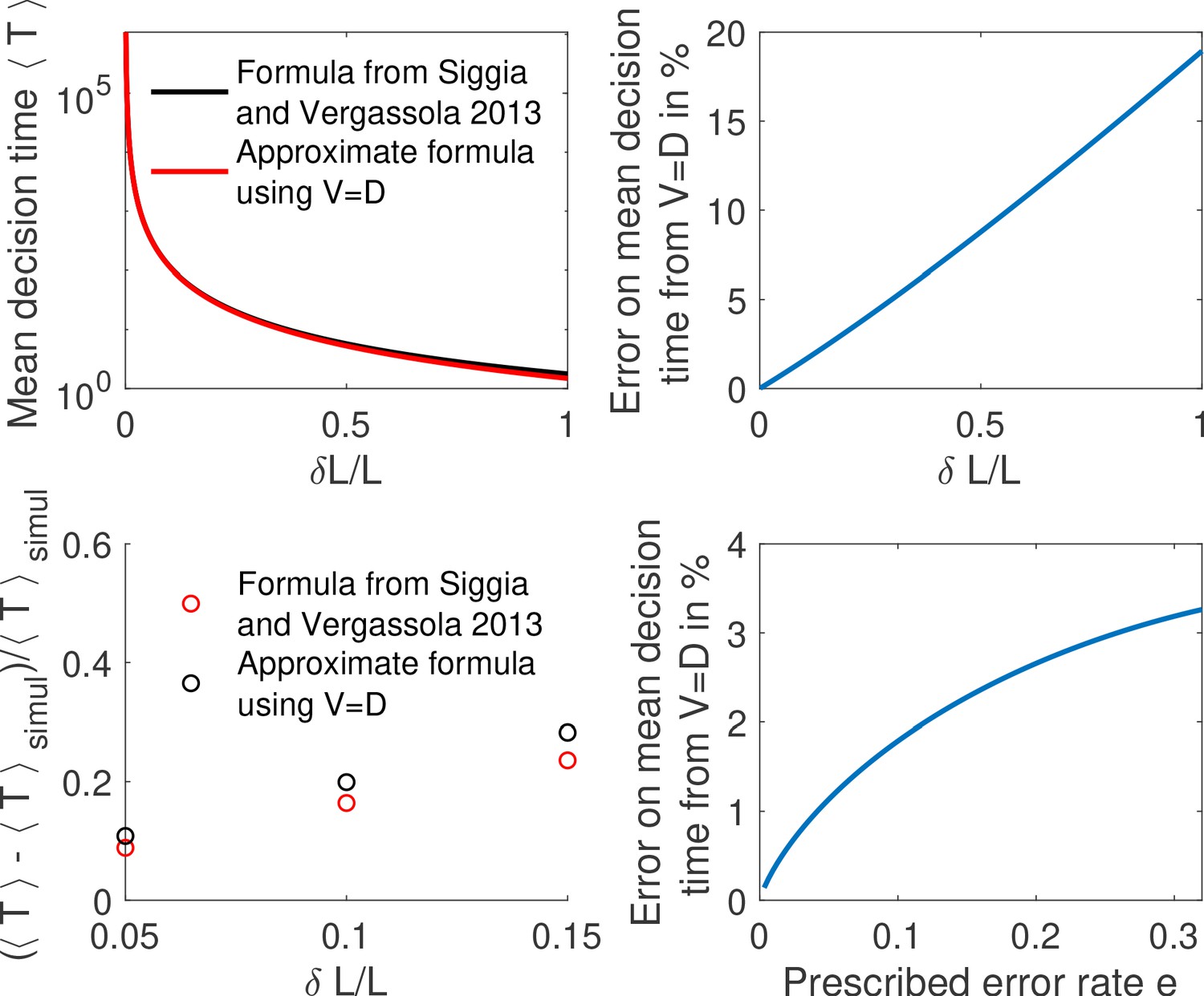
Comparing methods to compute the mean decision time for the one binding site case.

(a) We compute the mean decision time for one binding site using the method from Siggia and Vergassola, 2013 ${⟨ T ⟩}_{SV}$ (i.e ${⟨ T ⟩}_{SV} = K tanh (V K / 2 D) / V$ , Equation 2 from main text and Equation 26) in black and mean decision time $⟨ T ⟩$ from the approximate method using $V = D$ , Equation 2 and Equation 4 from main text in red. In panel (b) we show for the same results the error made from using $V = D : 100 * | ⟨ T ⟩_{S V} - ⟨ T ⟩ | / ⟨ T ⟩_{S V}$ . We find that the difference is small for small concentration differences $δ L / L$ . (c) We show the relative error for the methods to compute the mean decision time compared to the mean time to decision ${⟨ T ⟩}_{simul}$ in a Monte-Carlo simulation. We find again that the error is small for small concentration differences. Parameters are $e = 0.32$ , $L = L_{2} = 1 μ m^{- 3}$ , $L_{1} = L + δ L$ , $μ = 1 μ m^{3} s^{- 1}$ , $ν = 1 s^{- 1}$ . (d) We show the relative error from $V = D$ (i.e $100 * | {⟨ T ⟩}_{SV} - ⟨ T ⟩ | / {⟨ T ⟩}_{SV}$ ) for fixed $δ L / L = 0.2$ as a function of the error rate. We find that the correction to $V = D$ is weak for small errors. Other parameters are the same as a,b,c.

Appendix 3—figure 3

Download asset Open asset

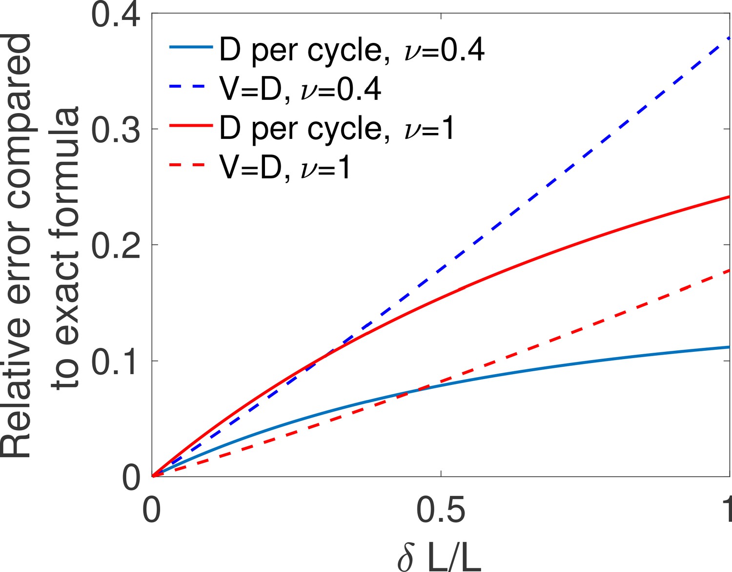
Comparing two approximations for the diffusivity.

For different values of the relative difference in concentrations $δ L / L$ and for one binding site with ON rate $μ L$ and OFF rate ν, we compute the mean time to decision using the exact formula from Siggia and Vergassola, 2013 ${⟨ T ⟩}_{SV}$ (computing D according to Equation 26), the mean time to decision computing D as a variable per cycle as in Equation 39 ${⟨ T ⟩}_{pc}$ and the mean time per cycle using $V = D ⟨ T ⟩$ . We show for both the per cycle (full lines) and the $V = D$ (dotted lines) method, the relative error made in computing the mean decision time by comparing it to the exact time ${⟨ T ⟩}_{SV}$ . We find that all methods agree for small $δ L / L$ , but that the per cycle method is a better approximation only for small values of the OFF rate ν (blue curves), i.e when the times do not depend strongly on the concentration. Parameters are $e = 0.32$ , $L = L_{2} = 1 μ m^{- 3}$ , $L_{1} = L + δ L$ , $μ = 1 μ m^{3} s^{- 1}$ .

Appendix 4—figure 1

Download asset Open asset

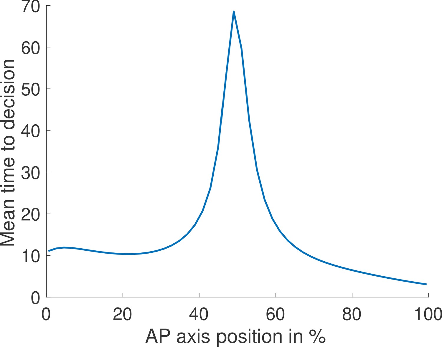
Mean time to decision across the embryo based on local Bicoid concentration difference.

For each position across the embryo, we compute the performance of the fastest identified architecture ( $k = 1$ , no Hill coefficient constraint) if it was implemented to distinguish between two concentrations with 10% relative variation, and an average equal to the Bicoid concentration at the AP position denoted on the x-axes. We find that our architecture performs well in the anterior region but is slow in the posterior region, due to low concentrations.

Appendix 4—figure 2

Download asset Open asset

Mean time to decision across the embryo assuming fixed thresholds and log-likelihood functions.

We compute for each position along the embryo the mean time to decision for the fastest architecture identified with $k = 1$ and no Hill coefficient constraints. We assume one biological mechanism for the readout meaning that, at every position, the log-likelihood of the waiting times are computed using the same function (one function across the embryo for the ON times and one for the OFF times). This function is determined by the log-likelihoods at the two edges of the mid-embryo region because it is the hardest discrimination task. The thresholds corresponding to deciding for anterior and posterior are also fixed throughout the embryo. We find that our model predicts that nuclei located close to the boundary take more time to trigger a decision.

Appendix 5—figure 1

Download asset Open asset

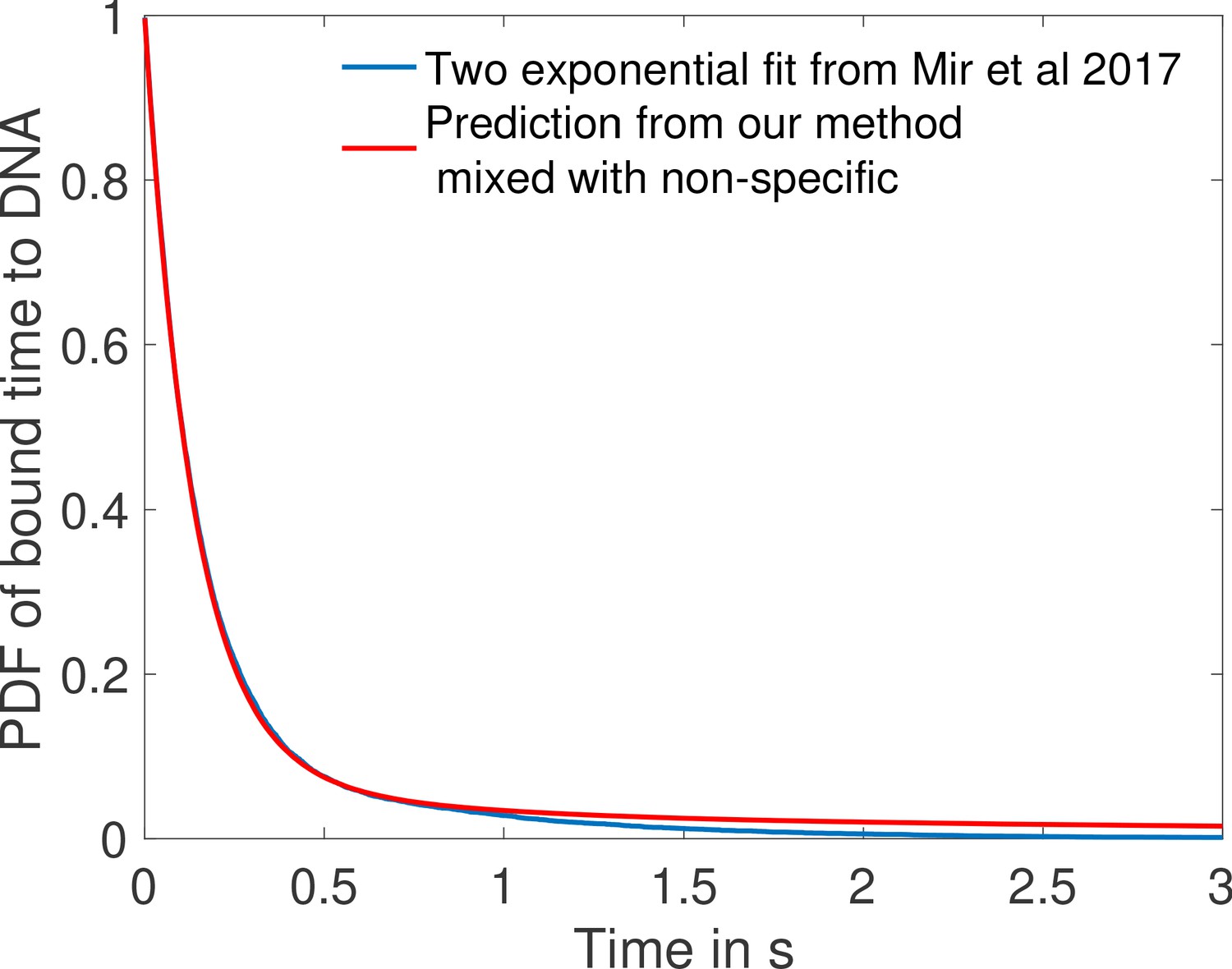
Comparison of fit to data from Mir et al., 2017 and prediction from one of the fastest architectures for time spent bound to DNA by Bicoid molecules.

In blue we show the two exponential fit for the pdf of the time spent bound to the DNA by Bicoid molecules at the boundary for the Zelda null conditions in Mir et al., 2017. They fit two exponentials to the data obtaining a coefficient of determination above 0.99 for a least square fit. Their fit finds 12.9% specific traces with mean 0.629 s and 87.1% non-specific traces with mean 0.131 s. In blue we show the PDF of time spent bound to DNA for a mix of 87.1% non-specific traces with the same mean 0.131 s and 12.9% specific traces drawn from the distribution of time spent to DNA based on the fastest promoter architecture identified for $k = 2$ , $H > 5$ (obtained from Monte Carlo simulation). Our prediction fits the blue curve from Mir et al., 2017 with a coefficient of determination above 0.99 as well.

Appendix 7—figure 1

Download asset Open asset

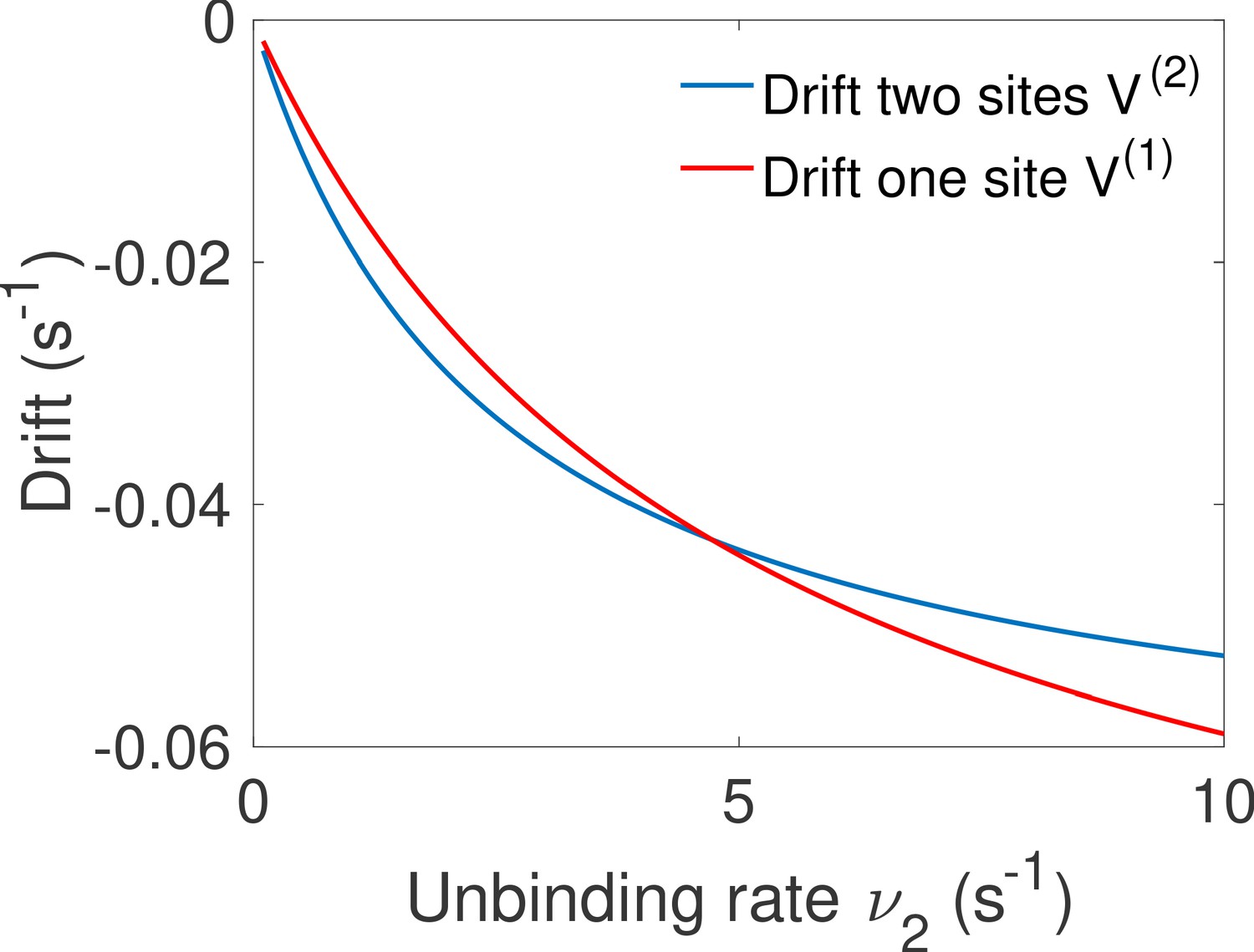
Comparison of the drift for the one and two binding site equilibrium architectures.

We compare the drift $V^{(1)}$ of the one binding-site architecture of Main Text Figure 5d and the drift $V^{(2)}$ for the two binding site equilibrium architecture of Main Text Figure 5c. Both have the same parameters $L = L_{2} = 1 μ m^{- 3}$ , $L_{1} = 1.1 μ m^{- 3}$ , $μ_{1} = μ_{2} = 5 μ m^{3} s^{- 1}$ , $ν_{1} = 5 s^{- 1}$ and we vary $ν_{2}$ . The fastest architecture is the one with the highest absolute value of the drift (lowest on the graph). We recover the transition observed in Main Text Figure 5f between the optimal architectures.

Appendix 7—figure 2

Download asset Open asset

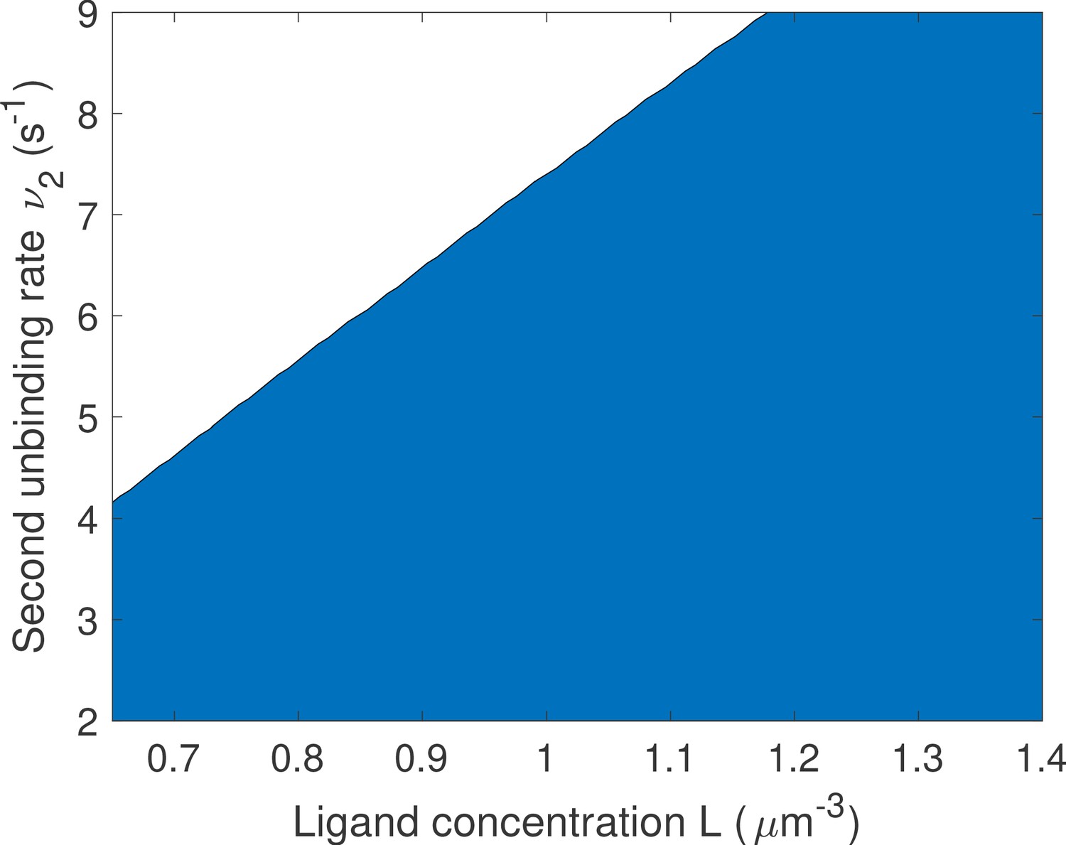
Changing the bounds of the rates does not change the qualitative results on the optimal number of binding sites.

We proceed as in Main Text Figure 5f: for a given value of L and ν we compare one- and two-binding site architectures. The blue region corresponds to two binding site promoter being optimal and the white region to one binding site promoter being optimal. Parameters are the same as in Main Text Figure 5f except that the upper bounds for μ₁ and μ₂ are increased to $5 μ m^{3} s^{- 1}$ and that of ν₁ is increased to $5.5 s^{- 1}$ . We find that the results are qualitatively similar to that of Main Text Figure 5f. although the transition to optimal one binding site region is shifted up.

Appendix 9—figure 1

Download asset Open asset

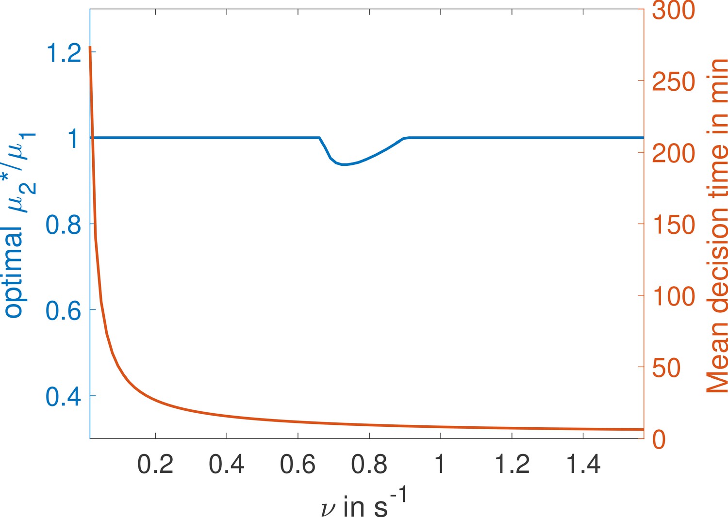
Weak binding sites are optimal for a range of parameters.

In the $k = 1$ , two binding site cycle architecture of Main Text Figure 5c, we fix ν and L and optimize for second binding rate μ₂ for a given value of μ₁, imposing $μ_{2} \leq μ_{1}$ . We identify the value $μ_{2}^{*}$ for which the architecture is fastest and plot the ratio $μ_{2}^{*} / μ_{1}$ . We find that for certain values of ν the second binding is not as fast as it could be, corresponding to a weaker binding site (binding probability is below one and the ON rate is below the diffusion limit). Parameters are $L = 0.5 μ m^{- 3}$ , $L_{2} = L$ , $L_{1} = 0.9 L$ , $e = 5 %$ , $μ_{1} = 1 μ m^{3} s^{- 1}$ .

Appendix 11—figure 1

Download asset Open asset

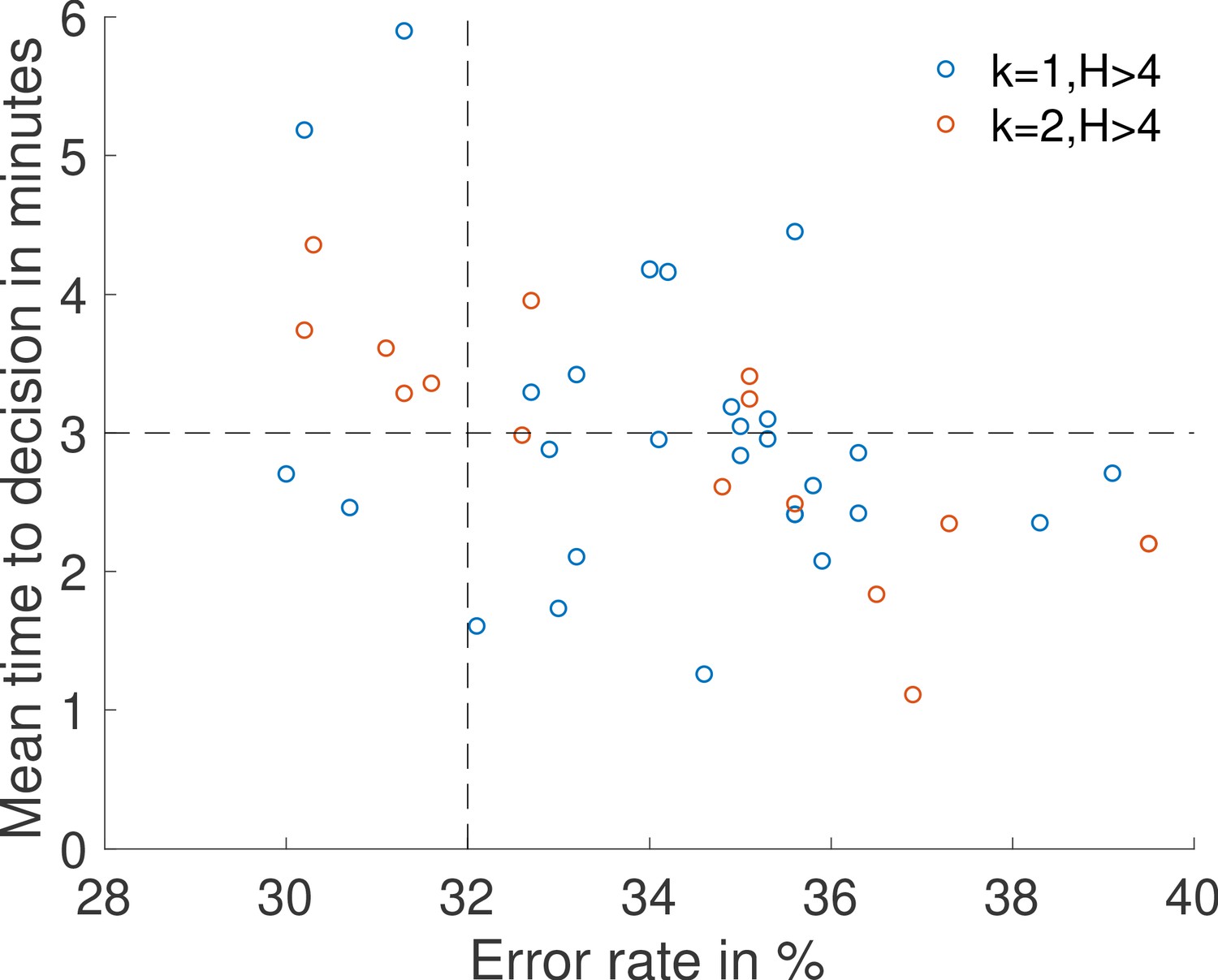
Results of a search for sets of parameters $r_{ON}$ , $r_{OFF}$ , $r_{b}$ , $d_{ON}$ , $d_{OFF}$ , $c_{1}$ and $c_{2}$ that lead to an accurate decision ( $e < 32 %$ ) in a short time ( $⟨ T ⟩ < 180 s$ ).

The ON and OFF times are drawn from the fastest architectures identified with rules $k = 1$ , $H > 4$ (blue dots) and $k = 2$ , $H > 4$ (red dots). Concentrations are $L_{1} = 1.05 L_{0}$ and $L_{2} = 0.95 L_{0}$ .

Appendix 12—figure 1

Download asset Open asset

Computing gene ON and OFF times statistics for the enhancer dynamics.

We check that our analytical method (see Appendix 12) properly predicts the ON (a) and OFF (b) waiting time PDF for the gene assuming a seven state promoter and a two state enhancer with independent dynamics and a gene that is ON when both the promoter and enhancer are ON. Parameters are $L = 1 μ m^{- 3}$ , ${(μ_{i})}_{1 \leq i \leq 6} = (0.2, 0.8, 0.15, 0.4, 1.2, 0.7) s^{- 1}$ , ${(ν_{i})}_{1 \leq i \leq 6} = (1.3, 0.2, 0.4, 0.6, 0.7, 0.8) s^{- 1}$ , $e_{ON} = 0.2 s^{- 1}$ , $e_{OFF} = 0.6 s^{- 1}$ .

Tables

Appendix 1—table 1

Mean decision times for various choices of parameters and four different decision processes (see sections 'Biological parameters in the embryo' and 'Error rate and decision time for the fixed-time decision strategy').

For the optimal architectures identified (third and fourth lines of the table) we take the fastest architectures without any constraints on the slope. These architectures systematically use the activation rule $k = 1$ . Highlighted in red are the results for the range of parameters presented in the text. All calculations are made with $e = 32 %$ , $L = L_{1} = 1.05 \cdot L_{0}$ , $L_{2} = 0.95 \cdot L_{0}$ . The diffusion limited ON rate is $μ_{max} L_{0} = D a L_{0}$ . For the two Berg-Purcell architectures, both the ON rate and OFF rate per site are equal to $μ_{max}$ . For the optimal architectures, we have $μ_{i} L_{0} = μ_{max} L_{0} \cdot (7 - i)$ and $ν_{i} = i \cdot μ_{max} L_{0} \cdot {0.5}^{1 / 6} / (1 - {0.5}^{1 / 6})$ to keep half the genes active at the boundary.

	$a_{1}$				$a_{2}$
	$D_{1}$		$D_{2}$		$D_{1}$		$D_{2}$
	$L_{0}^{(1)}$	$L_{0}^{(2)}$	$L_{0}^{(1)}$	$L_{0}^{(2)}$	$L_{0}^{(1)}$	$L_{0}^{(2)}$	$L_{0}^{(1)}$	$L_{0}^{(2)}$
Berg-Purcell one operator site	4.0 hr	100 min	117 min	59 min	20 min	10 min	12 min	5.9 min
Berg-Purcell twelve operator sites independently read	58 min	29 min	34 min	17 min	5.8 min	2.9 min	3.4 min	1.7 min
Optimal equilibrium architecture fixed-time decision ( $e = 0.32$ )	24 min	13 min	15 min	7.7 min	2.8 min	1.6 min	1.8 min	1.1 min
Optimal equilibrium architecture SPRT decision ( $e = 0.32$ )	17 min	8.5 min	9.9 min	5.0 min	1.7 min	51 s	1.0 min	30 s

Additional files

Source code 1 Search for optimal architectures.: https://cdn.elifesciences.org/articles/49758/elife-49758-code1-v2.zip
Download elife-49758-code1-v2.zip
Transparent reporting form: https://cdn.elifesciences.org/articles/49758/elife-49758-transrepform-v2.docx
Download elife-49758-transrepform-v2.docx

Download links

A two-part list of links to download the article, or parts of the article, in various formats.

Downloads (link to download the article as PDF)

Article PDF

Open citations (links to open the citations from this article in various online reference manager services)

Mendeley

Cite this article (links to download the citations from this article in formats compatible with various reference manager tools)

Jonathan Desponds
Massimo Vergassola
Aleksandra M Walczak

(2020)

A mechanism for hunchback promoters to readout morphogenetic positional information in less than a minute

eLife 9:e49758.

https://doi.org/10.7554/eLife.49758

Share this article

Cite this article

Decision between anterior and posterior developmental blueprints.

The relation between promoter structure and on-the-fly decision-making.

Comparing the performance of two promoter activation rules.

Performance, constraints and statistics of fastest decision-making architectures.

The effects of different promoter architectures on the mean decision time.

Predictions for experiments with synthetic hb promoters.

A model of RNA production and degradation approximates the contributions to log-likelihood.

The mean decision time as a function of the error rate e for the fastest architecture identified with H>5 and k=1 (see Main Text Figure 4a).

The equality V=D holds for close hypotheses.

Comparing methods to compute the mean decision time for the one binding site case.

Comparing two approximations for the diffusivity.

Mean time to decision across the embryo based on local Bicoid concentration difference.

Mean time to decision across the embryo assuming fixed thresholds and log-likelihood functions.

Comparison of fit to data from Mir et al., 2017 and prediction from one of the fastest architectures for time spent bound to DNA by Bicoid molecules.

Comparison of the drift for the one and two binding site equilibrium architectures.

Changing the bounds of the rates does not change the qualitative results on the optimal number of binding sites.

Weak binding sites are optimal for a range of parameters.

Results of a search for sets of parameters rON, rOFF, rb, dON, dOFF, c1 and c2 that lead to an accurate decision (e<32%) in a short time (⟨T⟩<180s).

Computing gene ON and OFF times statistics for the enhancer dynamics.

Mean decision times for various choices of parameters and four different decision processes (see sections 'Biological parameters in the embryo' and 'Error rate and decision time for the fixed-time decision strategy').

Source code 1

Transparent reporting form

Downloads (link to download the article as PDF)

Open citations (links to open the citations from this article in various online reference manager services)

Cite this article (links to download the citations from this article in formats compatible with various reference manager tools)

The mean decision time as a function of the error rate e for the fastest architecture identified with $H > 5$ and $k = 1$ (see Main Text Figure 4a).

The equality $V = D$ holds for close hypotheses.

Results of a search for sets of parameters $r_{ON}$ , $r_{OFF}$ , $r_{b}$ , $d_{ON}$ , $d_{OFF}$ , $c_{1}$ and $c_{2}$ that lead to an accurate decision ( $e < 32 %$ ) in a short time ( $⟨ T ⟩ < 180 s$ ).