Categorical representation from sound and sight in the ventral occipito-temporal cortex of sighted and blind
- Institute of research in Psychology (IPSY) & Institute of Neuroscience (IoNS) - University of Louvain (UCLouvain), Belgium
- Centre for Mind/Brain Sciences, University of Trento, Italy
Figures
Figure 1 with 1 supplement
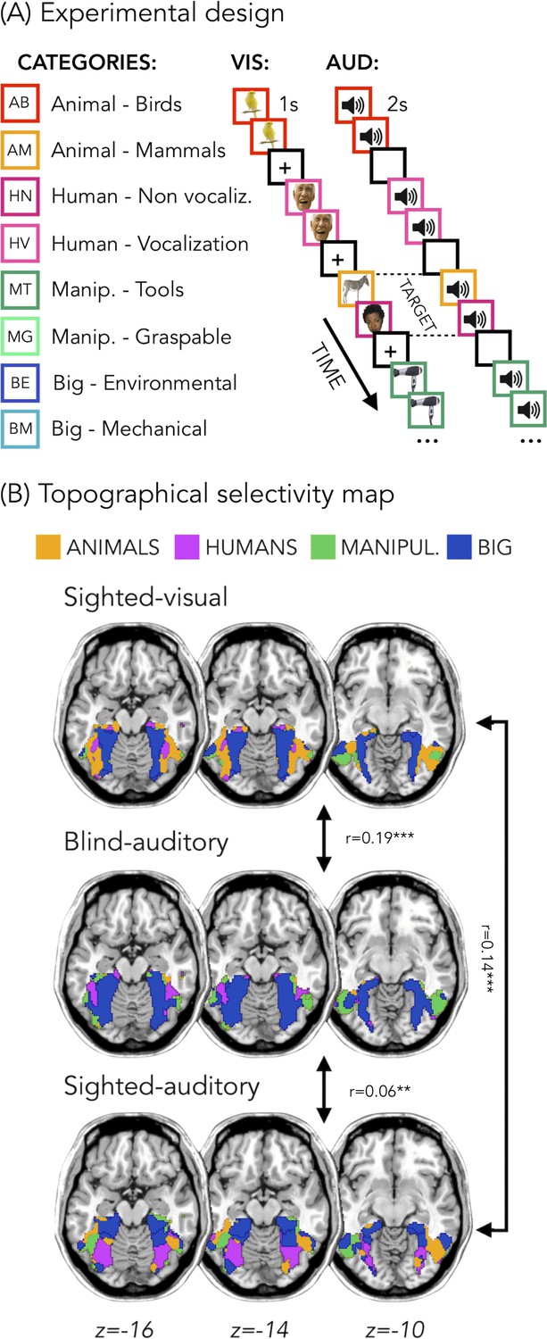
Experimental design and topographical selectivity maps.
(A) Categories of stimuli and design of the visual (VIS) and auditory (AUD) fMRI experiments. (B) Averaged untresholded topographical selectivity maps for the sighted-visual (top), the blind-auditory (center) and the sighted-auditory (bottom) participants. These maps visualize the functional topography of VOTC to the main four categories in each group. These group maps are created for visualization purpose only since statistics are run from single subject maps (see methods). To obtain those group maps, we first averaged the β-values among participants of the same group in each voxel inside the VOTC mask for each of our 4 main conditions (animals, humans, manipulable objects and places) separately and we then assign to each voxel the condition producing the highest β-value. We decided to represent maps including the 4 main categories (instead of 8) to simplify visualization of the main effects (the correlation values are almost identical with 8 categories and those maps can be found in supplemental material).
Figure 1—figure supplement 1
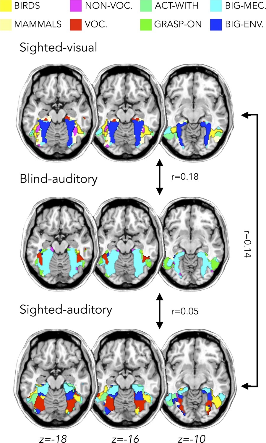
Topographical selectivity map for 8 categories.
The averaged untresholded topographical selectivity maps for the sighted-visual (top), the blind-auditory (center) and the sighted-auditory (bottom) participants. These maps visualize the functional topography of VOTC to the eight sub-categories. The average correlation between each group comparison is reported.
Figure 2 with 1 supplement
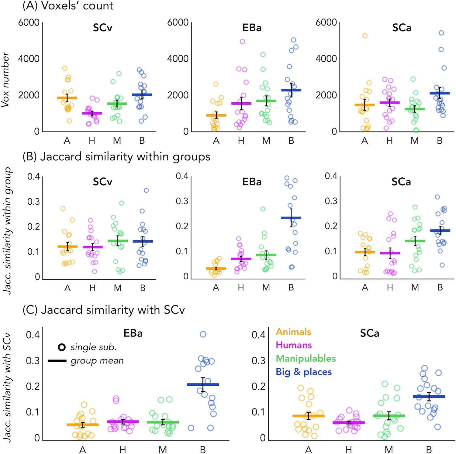
Voxels’ count and Jaccard analyses.
(A) Number of selective voxels for each category in each group, within VOTC. Each circle represents one subject, the colored horizontal lines represent the group average and the vertical black bars are the standard error of the mean across subjects. (B) The Jaccard similarities values within each group, for each of the four categories. (C) The Jaccard similarity indices between the EBa and the SCv groups (left side) and the Jaccard similarity indices between the SCa and the SCv groups (right side).
Figure 2—figure supplement 1
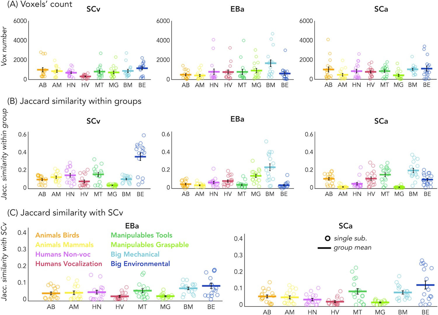
Voxels’ count and Jaccard analyses for eight categories.
Results on the eight sub-categories from the selective voxels’ count for each category (first line); from the Jaccard similarity analysis within each group (middle line); from the Jaccard similarity with SCv (bottom line). Each circle represents one subject, the colored horizontal line represents the group mean and the black vertical bars represent the standard error of the mean across subjects.
Figure 3
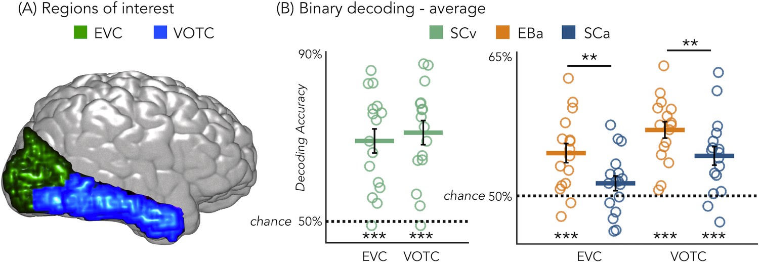
Regions of interest and classification results.
(A) Representation of the 2 ROIs in one representative subject’s brain; (B) Binary decoding averaged results in early visual cortex (EVC) and ventral occipito-temporal cortex (VOTC) for visual stimuli in sighted (green), auditory stimuli in blind (orange) and auditory stimuli in sighted (blue). ***p<0.001, **p<0.05.
Figure 4
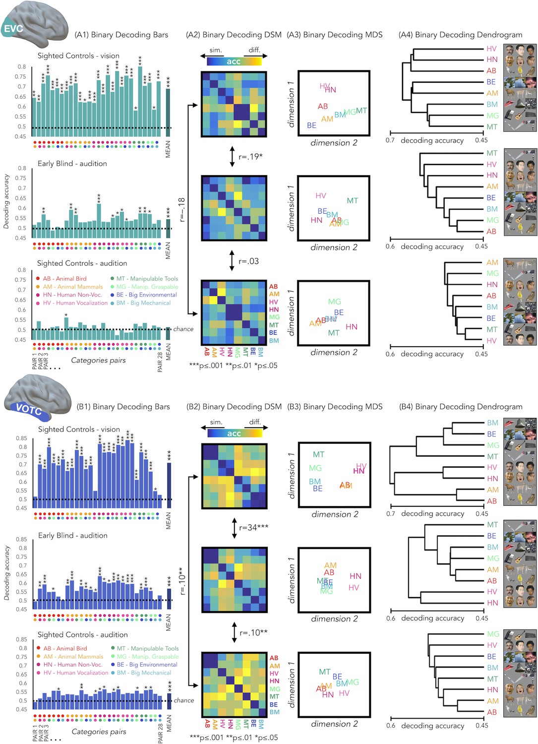
EVC and VOTC functional profiles.
(A1 and B1) Binary decoding bar plots. For each group (SCv: top; EBa: center; SCa: bottom) the decoding accuracy from the 28 binary decoding analyses are represented. Each column represents the decoding accuracy value coming from the classification analysis between 2 categories. The 2 dots under each column represent the 2 categories. (A2 and B2) The 28 decoding accuracy values are represented in the form of a dissimilarity matrix. Each column and each row of the matrix represent one category. In each square there is the accuracy value coming from the classification analysis of 2 categories. Blue color means low decoding accuracy values and yellow color means high decoding accuracy values. (A3 and B3) Binary decoding multidimensional scaling (MDS). The categories have been arranged such that their pairwise distances approximately reflect response pattern similarities (dissimilarity measure: accuracy values). Categories placed close together were based on low decoding accuracy values (similar response patterns). Categories arranged far apart generated high decoding accuracy values (different response patterns). The arrangement is unsupervised: it does not presuppose any categorical structure (Kriegeskorte et al., 2008b). (A4 and B4) Binary decoding dendrogram. We performed hierarchical cluster analysis (based on the accuracy values) to assess if EVC (A4) and VOTC (B4) response patterns form clusters corresponding to natural categories in the 3 groups (SCv: top; EBa: center; SCa: bottom).
Figure 5 with 1 supplement

Hierarchical clustering of brain data: VOTC and EVC.
Hierarchical clustering on the dissimilarity matrices extracted from EVC (left) and VOTC (right) in the three groups. The clustering was repeated three times for each DSM, stopping it at 2, 3 and 4 clusters, respectively. This allows to compare the similarities and the differences of the clusters at the different steps across the groups. In the figure each cluster is represented in a different color. The first line represents 2 clusters (green and red); the second line represents 3 clusters (green, red and pink); finally, the third line represents 4 clusters (green, red, pink and light blue).
Figure 5—figure supplement 1
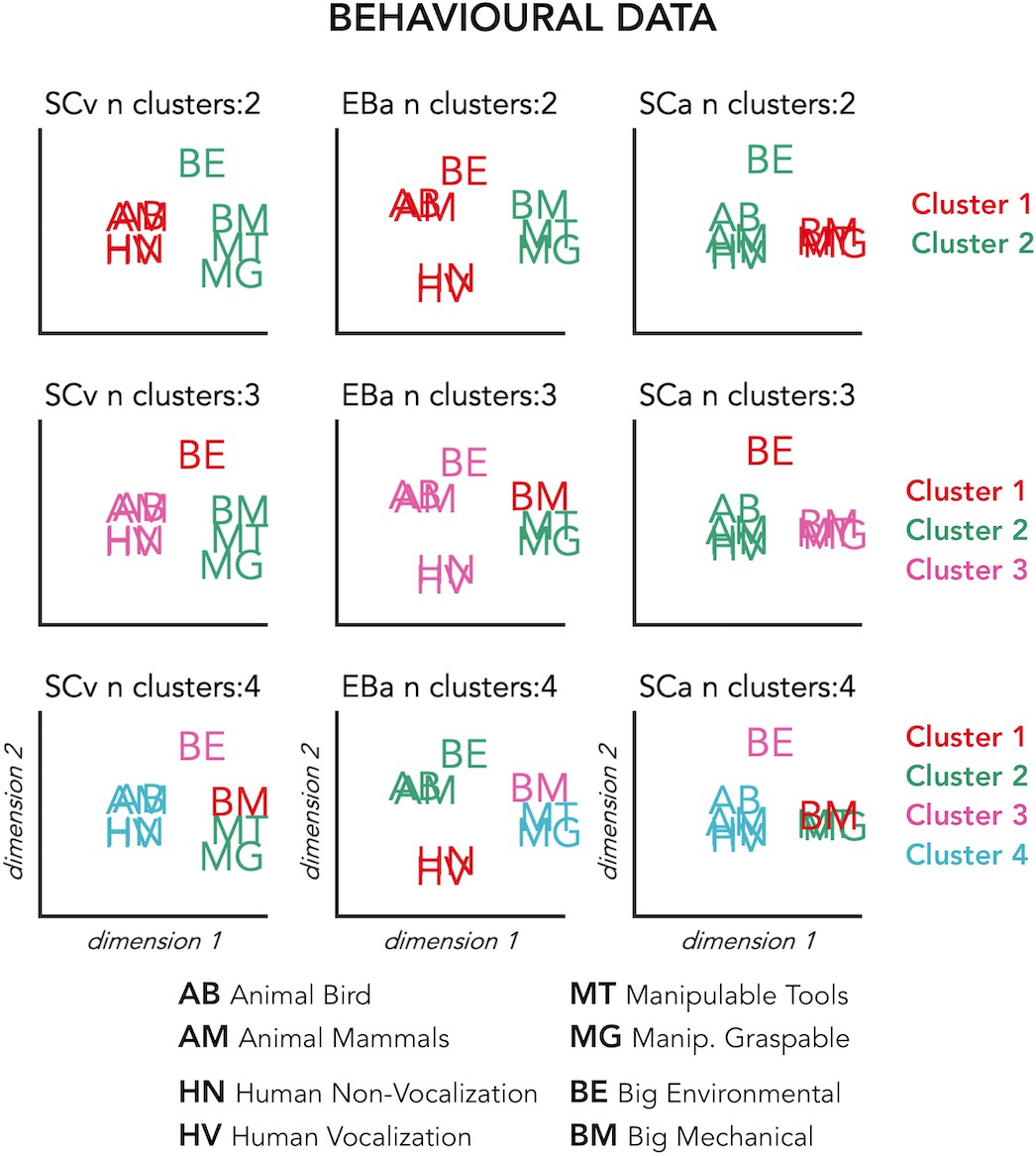
Hierarchical clustering of the behavioral data.
Hierarchical clustering on the dissimilarity matrices built from the behavioral ratings. The clustering was repeated three times for each DSM, stopping it at 2, 3 and 4 clusters, respectively. This allows to compare the similarities and the differences of the clusters at the different steps across the groups. In the figure each cluster is represented in a different color. The first line represents 2 clusters (green and red); the second line represents 3 clusters (green, red and pink); finally the third line represents 4 clusters (green, red, pink and light blue).
Figure 6 with 1 supplement
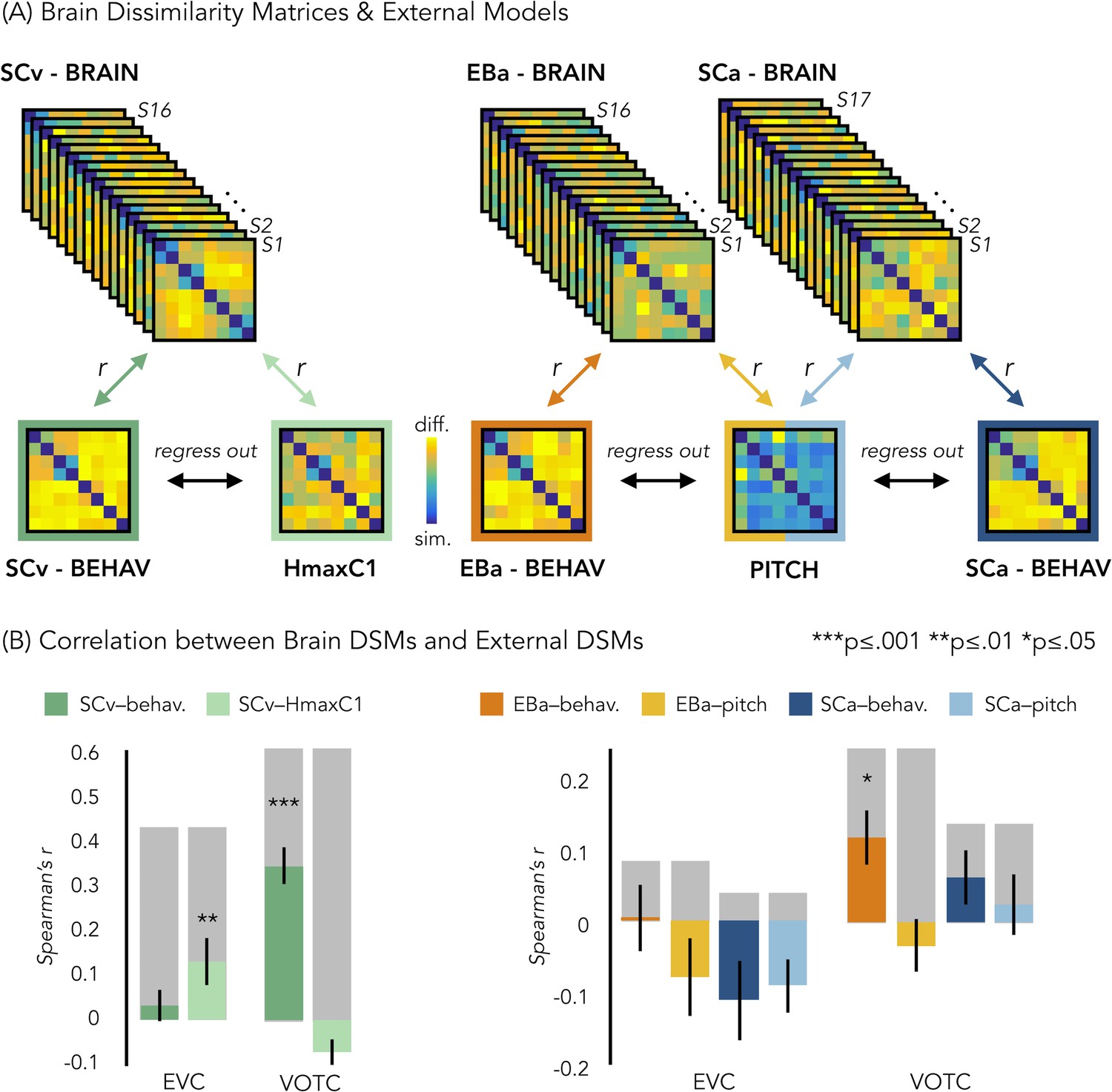
Representational similarity analysis (RSA) between brain and representational low-level/behavioral models.
(A) In each ROI we computed the brain dissimilarity matrix (DSM) in every subject based on binary decoding of our 8 different categories. In the visual experiment (left) we computed the partial correlation between each subject’s brain DSM and the behavioral DSM from the same group (SCv-Behav.) regressing out the shared correlation with the HmaxC1 model, and vice versa. In the auditory experiment (right) we computed the partial correlation between each subject’s brain DSM (in both Early Blind and Sighted Controls) and the behavioral DSM from the own group (either EBa-Behav. or SCa-Behav.) regressing out the shared correlation with the pitch model, and vice versa. (B) Results from the Spearman’s correlation between representational low-level/behavioral models and brain DSMs from both EVC and VOTC. On the left are the results from the visual experiment. Dark green: partial correlation between SCv brain DSM and behavioral model; Light green: Partial correlation between SCv brain DSM and HmaxC1 model. On the right are the results from the auditory experiment in both early blind (EBa) and sighted controls (SCa). Orange: partial correlation between EBa brain DSM and behavioral model; Yellow: Partial correlation between EBa brain DSM and pitch model. Dark blue: partial correlation between SCa brain DSM and behavioral model; Light blue: partial correlation between SCa brain DSM and pitch model. For each ROI and group, the gray background bar represents the reliability of the correlational patterns, which provides an approximate upper bound of the observable correlations between representational low-level/behavioral models and neural data (Bracci and Op de Beeck, 2016; Nili et al., 2014). Error bars indicate SEM. ***p<0.001, **p<.005, *p<0.05. P values are FDR corrected.
Figure 6—figure supplement 1
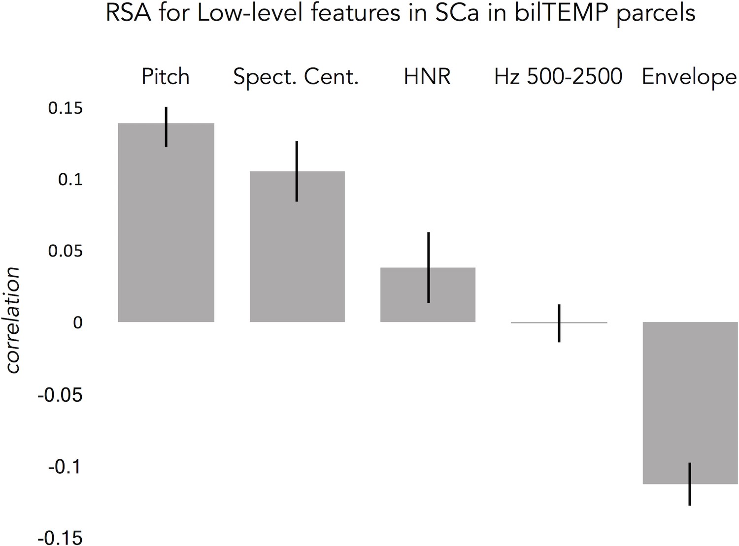
Auditory model selection.
To select the auditory model we tested different low-level acoustic models on the sighted participants that took part in the auditory experiment. The following models were tested: pitch; harmonicity to noise ratio (HNR); spectral centroid (S.Cent.); the voice frequency band (between 500–2500 Hz) and the sound energy per unit of time (envelope). We extracted these values from our 24 auditory stimuli and we built 5 dissimilarity matrices (DSM) each one based on one acoustic feature. Then, we extracted the brain dissimilarity matrix (1-Pearson’s correlation between each pattern of activity) from the auditory cortex of each sighted subject that took part in the auditory experiment. Here is represented the second-order correlation between each acoustic model and the brain DSMs, ranked from the highest to the lowest (left to right). Since pitch resulted the most represented model in the auditory cortex of sighted participants, we selected this acoustic model to run further analyses in the experiment.
Figure 7
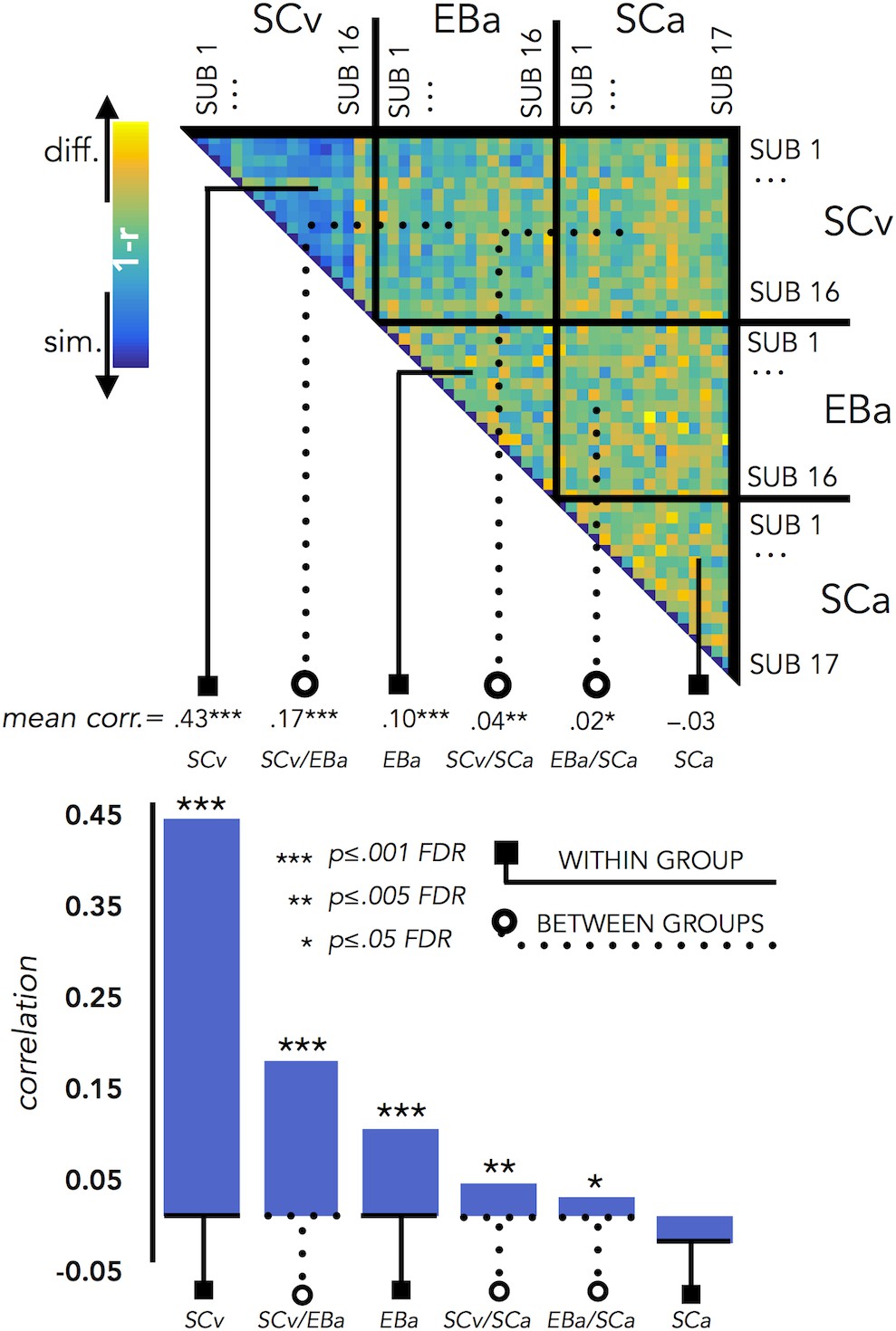
VOTC Inter-subject correlation within and between groups.
Upper panel represents the correlation matrix between the VOTC brain DSM of each subject with all the other subjects (from the same group and from different groups). The mean correlation of each within- and between-groups combination is reported in the bottom panel (bar graphs). The straight line ending with a square represents the average of the correlation between subjects from the same group (i.e. within groups conditions: SCv, EBa, SCa), the dotted line ending with the circle represents the average of the correlation between subjects from different groups (i.e. between groups conditions: SCv-EBa/SCv-SCa/EBa SCa). The mean correlations are ranked from the higher to the lower inter-subject correlation values.
Figure 8
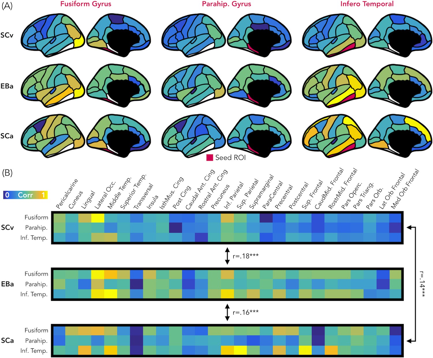
Representational connectivity.
(A) Representation of the z-normalized correlation values between the dissimilarity matrix of the three VOTC seeds (left: Fusiform gyrus, center: Parahippocampal gyrus, Right: Infero-Temporal cortex) and the dissimilarity matrix of 27 parcels covering the rest of the cortex in the three groups (top: SCv, central: EBa, bottom: SCa). Blue color represents low correlation with the ROI seed; yellow color represents high correlation with the ROI seed. (B) The normalized correlation values are represented in format of one matrix for each group. This connectivity profile is correlated between groups. SCv: sighted control-vision; EBa: early blind-audition; SCa: sighted control-audition.
Author response image 1
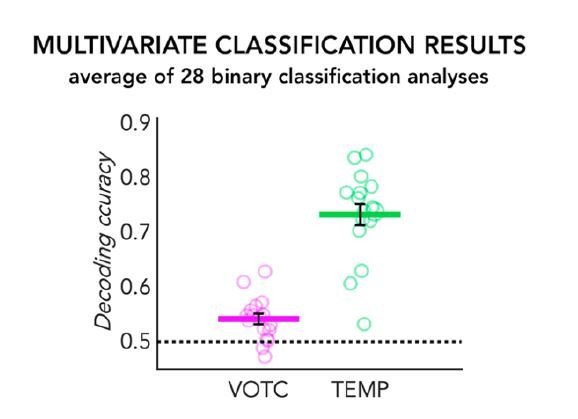
MVP-classification results in the SCa group.
The 28 binary classification accuracies averaged are represented for the VOTC (in pink) and the temporal ROI (in green). Each circle represents one subject, the coloured horizontal line represents the group mean and the black vertical bars represent the standard error of the mean across subjects.
Author response image 2
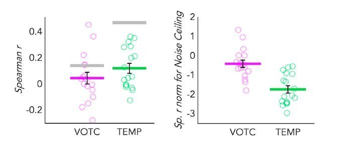
Dot-plot graphs representing the correlation of the behavioral model with the DSMs extracted from both VOTC (pink) and a TEMP (green) parcels, in sighted for auditory stimuli (SCa).
Each dot represents one subject, the colored (pink and green) lines represent the group mean values. The vertical black bars represent the standard error of the mean across subjects. Left panel: Spearman’s correlation with the behavioural model is represented here. The grey lines represent the noise ceiling (e.g. inter-subject correlation in each ROI). High inter-subject correlation means low variance. Right panel: The Spearman’s correlation values are represented after normalization for the noise ceiling. Since the noise ceiling was obviously higher than the group mean correlation in both ROI, negative values were expected after normalization.
Author response image 3
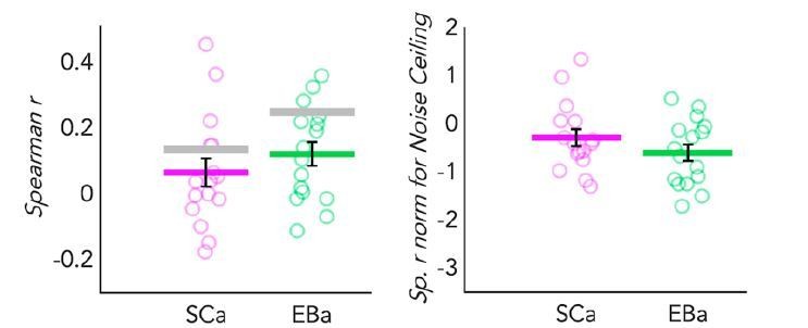
Dot-plot graphs representing the correlation of the behavioral model with the DSMs extracted from VOTC in both SCa (pink) and a EBa (green) groups.
Each dot represents one subject, the colored (pink and green) lines represent the group mean values. The vertical black bars represent the standard error of the mean across subjects. Left panel: Spearman’s correlation with the behavioural model. The grey lines represent the noise ceiling (e.g. inter-subject correlation in each group). High inter-subject correlation means low variance. Right panel: The Spearman’s correlation values are represented after normalization for the noise ceiling. Since the noise ceiling was higher than the group mean correlation in both group, negative values were expected after normalization.
Author response image 4
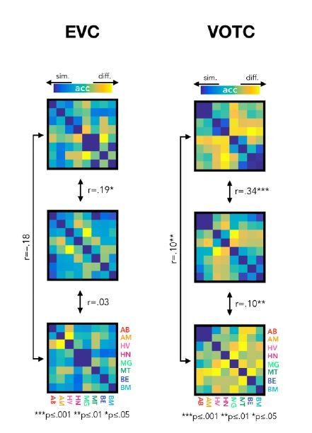
New version of the results from the correlation of brain DSMs in EVC (left) and in VOTC (right).
Despite a reduction of size effect in the new results, there is not any major change in the statistical results.
Author response image 5
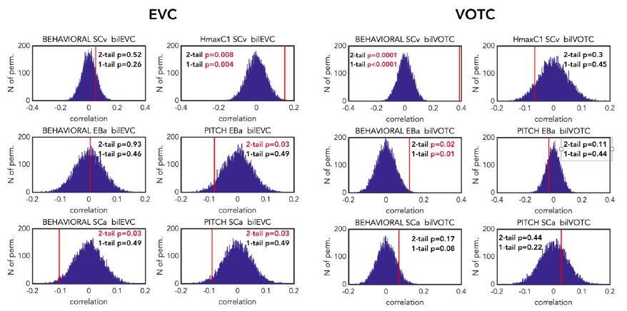
Comparison of the p-values (one-tailed vs two-tailed) resulting from the correlation of the brain DSMs (EVC on the left and VOTC on the right) with the representational behavioural and low-level models in the 3 groups (first line: SCv, middle line: EBa, lower line: SCa).
The null distribution is represented in dark blue. The red line represents the actual correlation value. For each permutation test p-values are reported both for two-tailed and one-tailed tests. P value reported in red are significant according to the selected threshold of 0.05. p values are reported after FDR correction for 12 multiple comparisons.
Author response image 6
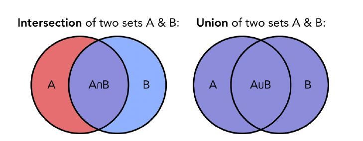
Visual representation of the intersection (left) and union (right) of two set of samples.
The Jaccard coefficient is based on these two measures.
Author response image 7
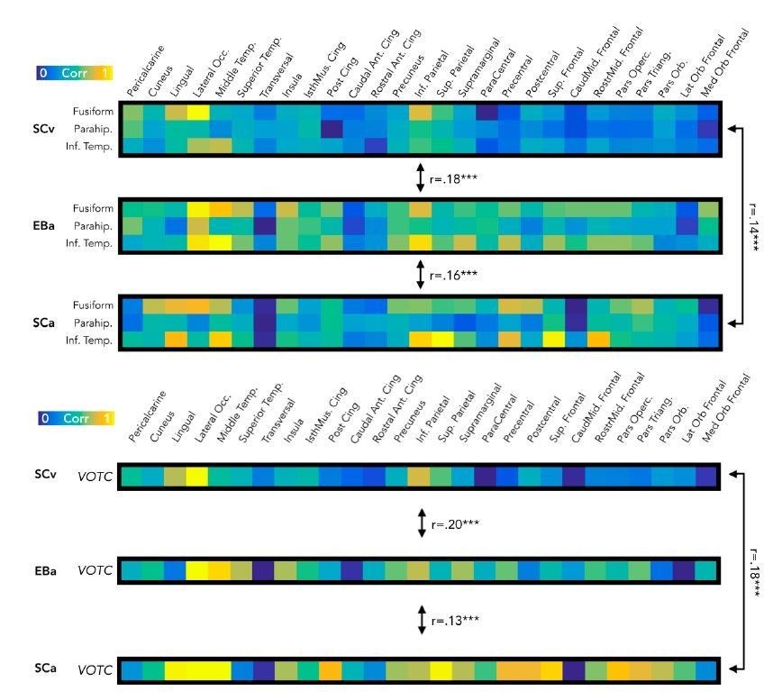
Comparisons of the results from the RSA connectivity analysis using the 3 sub-regions of VOTC (fusiform, parahippocampal, infero-temporal) as seeds ROIs or VOTC as a single ROI.
Additional files
-
Supplementary file 1
Categories and stimuli description.
- https://cdn.elifesciences.org/articles/50732/elife-50732-supp1-v2.docx
-
Supplementary file 2
Characteristics of early blind participants.
- https://cdn.elifesciences.org/articles/50732/elife-50732-supp2-v2.docx
-
Transparent reporting form
- https://cdn.elifesciences.org/articles/50732/elife-50732-transrepform-v2.docx
Download links
A two-part list of links to download the article, or parts of the article, in various formats.
Downloads (link to download the article as PDF)
Open citations (links to open the citations from this article in various online reference manager services)
Cite this article (links to download the citations from this article in formats compatible with various reference manager tools)
Categorical representation from sound and sight in the ventral occipito-temporal cortex of sighted and blind
eLife 9:e50732.
https://doi.org/10.7554/eLife.50732


