A model for focal seizure onset, propagation, evolution, and progression
- Department of Physiology and Cellular Biophysics, Columbia University, United States
- Department of Anesthesiology, NewYork-Presbyterian Hospital/Weill Cornell Medicine, United States
- Department of Neurology, Columbia University Medical Center, United States
- Department of Neurological Surgery, Columbia University Medical Center, United States
- Vagelos College of Physicians & Surgeons, Columbia University, United States
- Mortimer B. Zuckerman Mind Brain Behavior Institute, Department of Neuroscience, Columbia University, United States
Figures
Figure 1 with 1 supplement
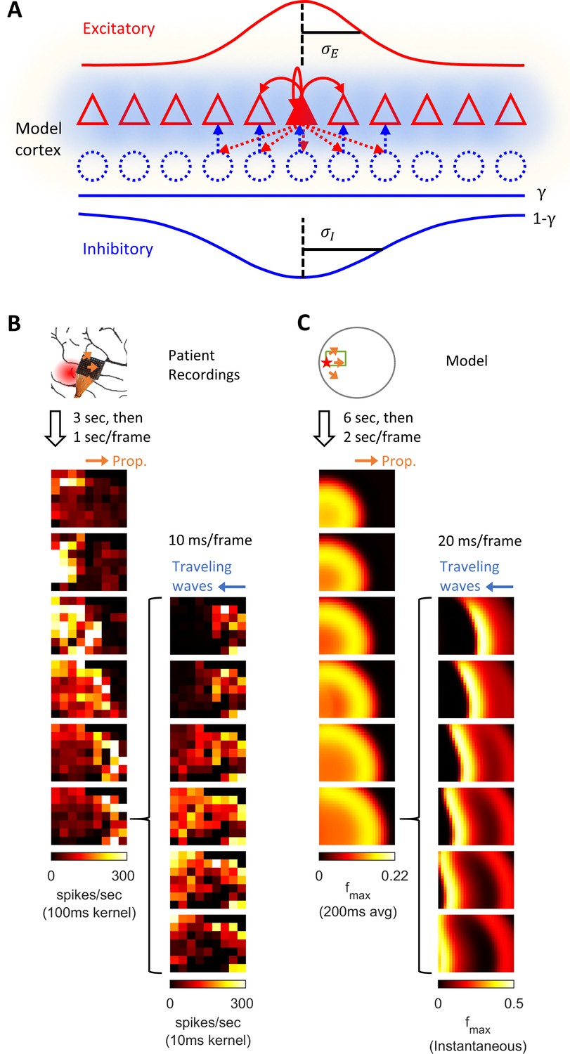
Model schematics and the comparison of patient recordings with model simulation results.
(A) Model schematic. Triangles: model neurons. Red solid arrows: excitatory recurrents with distance-dependent strength of spatial kernel width . Dashed blue circles: inhibitory neurons. Dashed red-to-blue arrows: distance-dependent di-synaptic recurrent inhibition with spatial kernel width , which accounts for of the total recurrent inhibition. The remaining fraction of the inhibition is distance independent and represented by the blue hues around model neurons. Interneuron membrane potentials are not explicitly modelled. (B) Microelectrode array recordings from Patient A. The red shaded area in the cartoon panel represents the clinically identified seizure onset zone. Orange arrows indicate the seizure propagation direction. The left column shows the spatiotemporal dynamics of multiunit activity in a slow timescale. The right column is a fast timescale zoom-in of the left bottom panel. Evolution of multiunit activity in a slow/fast timescale is estimated by convolving the multiunit spike trains with a 100/10 ms Gaussian kernel respectively. Left-to-right seizure recruitment was seen 3 s after the seizure onset (the orange arrow). Once recruited (left bottom panel), fine temporal resolution panels (the right column) showed right-to-left fast waves arose at the edge of the seizure territory (the blue arrow) and traveled toward the internal domain (fast inward traveling waves). (C) 2D rate model simulation results. Figure conventions adopted from B. The red star indicates where the seizure-initiating external current input was given (Id = 200 pA, duration 3 s, covering a round area with radius 5% of the whole neural sheet). Evolution of the neuronal activities within the green rectangle are shown in the panels. Notice the slow outward advancement of the seizure territory and the fast-inward traveling waves.
Figure 1—video 1
Full evolution of the model seizure shown in Figure 1C.
Figure 2 with 4 supplements
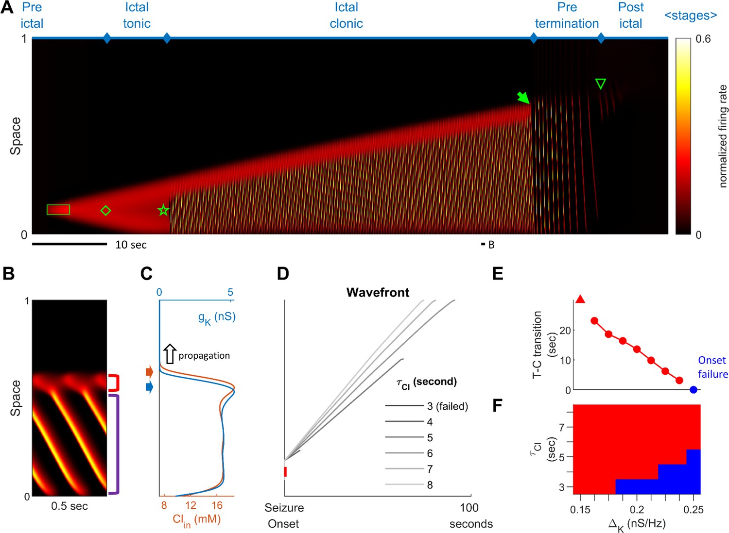
Stages of focal seizure evolution in a 1D rate model.
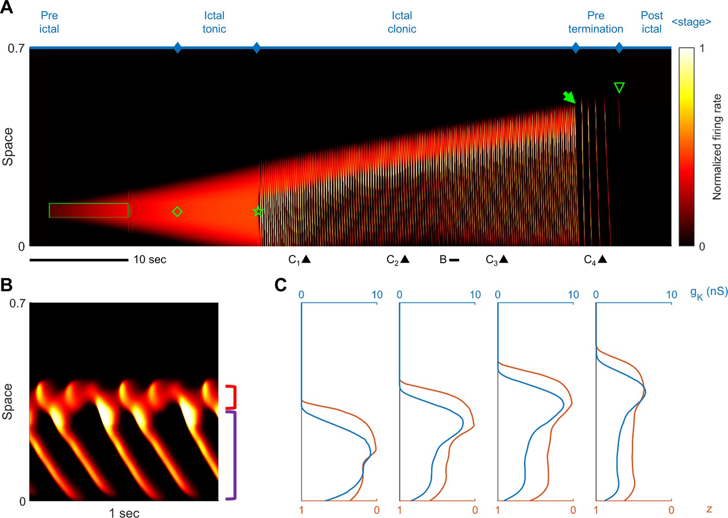
(A) Spatiotemporal evolution of a model seizure in one-dimensional space (EL=-57.5 mV). Horizontal axis: time; vertical-axis: space. Seizure dynamics is partitioned into the following distinct stages: pre-ictal, ictal-tonic, ictal-clonic, pre-termination, and post-ictal. Green box: seizure-provoking input (Id=200 pA). Green diamond: establishment of external-input-independent tonic-firing area. Green star: tonic-to-clonic transition. Green arrow: annihilation of the ictal wavefront. Green triangle: seizure termination. (B) Temporal zoom-in from Panel A during the ictal-clonic stage. Seizure territory further subdivided. Red square bracket: the ictal wavefront. Purple square bracket: the internal bursting domain. Thus, the top/bottom of the space corresponds to outside/inside of the seizure territory. Note that the fast-moving traveling waves move inwardly. Speed: 1.36 normalized space unit per second. Propagation speed of the ictal wavefront: 0.008 normalized space unit per second, for a traveling wave:wavefront speed ratio of 170. (C) Intracellular chloride concentration and sAHP conductance as a function of spatial position during the ictal-clonic stage, corresponding to the activity depicted in panel B. Note the distinct spatial fields of the two processes near the ictal wavefront. (D) Impaired chloride clearance allows seizure initiation and speeds up seizure propagation. Gray lines: the expansion of border of the seizure territory versus time. End of the lines: seizure termination, either spontaneous (τCl≤5 seconds) or after meeting the neural field boundary (τCl≥6 seconds). (E) Activation of the sAHP conductance leads to the tonic-to-clonic transition. Duration of ictal-tonic stage monotonously decreases as the sAHP conductance increases. Red triangle: persistent tonic stage without transition. (F) The seizure-permitting area in and parameter space. Blue/red: onset failure/success.
Figure 2—figure supplement 1
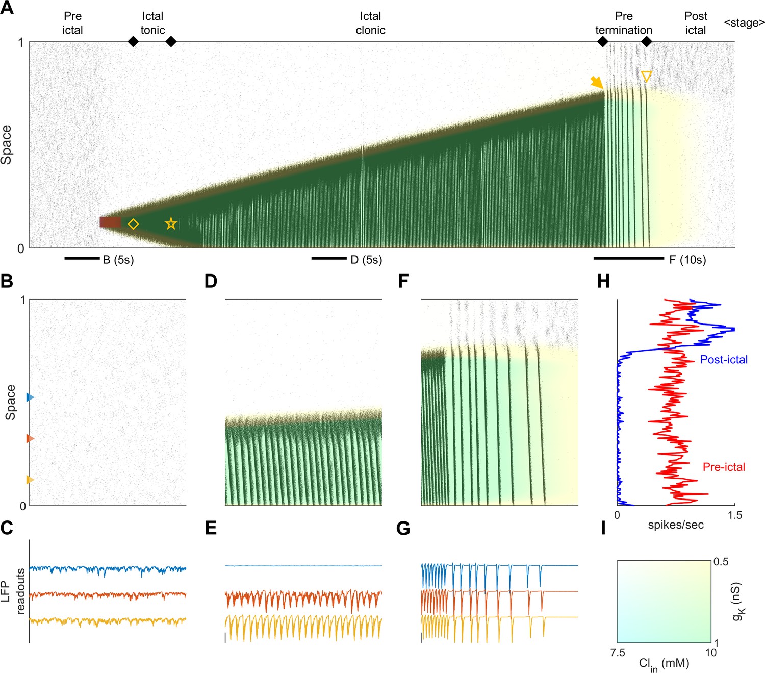
Stages of focal seizure evolution in a 1D spiking model.
(A) Spatiotemporal evolution of a model seizure simulated in a one-dimensional spiking neural network (model parameters: Table 2). Figure convention adopted from Figure 2A. Red shaded area: the seizure-provoking external excitatory input, =200 pA. Yellow diamond: establishment of the external input-independent tonic-firing area. Yellow star: tonic-to-clonic transition. Yellow arrow: annihilation of the ictal wavefront. Yellow triangle: seizure termination. The background colors represent the evolution of intracellular chloride concentration and sAHP conductance (see Panel I). (B) Temporal zoom-in during the pre-ictal stage. (C) LFP-like signal readouts, with the colors indicate where the signals are calculated in Panel B. (D) Temporal zoom-in during the ictal clonic-stage. The background color changes from the top to the bottom indicates accumulates first followed by sAHP upregulation. (E) LFP-like signal readouts of Panel D. Y-axis scale adjusted (10X than Panel C). (F) Temporal zoom-in during the pre-termination stage. (G) LFP-like signal readouts of Panel F. The seizure takes several seconds to slow down but still suddenly stops from the EEG perspective. (H) Neuronal firing rates comparison between pre-ictal (before applying the ictogenic stimulus) versus post-ictal periods (5 s, 10-neuron average). Notice the post-ictal suppression and the penumbra rebound excitation. (I) Reference color panel of and .
Figure 2—figure supplement 2

Effects of input triggers on model seizure dynamics.
(A) Spatiotemporal diagrams of network activity provoked by exogeneous excitatory stimuli. Green boxes: the spatiotemporal extents of the stimuli. Stimuli intensity: 100 pA. Stimulus durations: 1, 1.5, and 2 seconds from left the right respectively. Left: the network settles back to resting state immediately after the subthreshold stimulus. Middle: several afterdischarges are emitted after a near-threshold stimulus. Right: successful seizure onset. (B) High input currents, long duration, and large size focal inputs are more effective at triggering seizures. Successful seizure onset is defined if the activity of any rate unit is > 0.1 5 seconds after the end of the external input trigger. Parameter search was done over a logarithm scale grid. Minimal X-axis grid = 1 and Y-axis grid = 1/8. (C) Varying duration, size, and intensity of seizure-provoking inputs does not alter the sequence of seizure stages. The external inputs, are provided to the one-dimensional rate model at the center of the space.
Figure 2—figure supplement 3
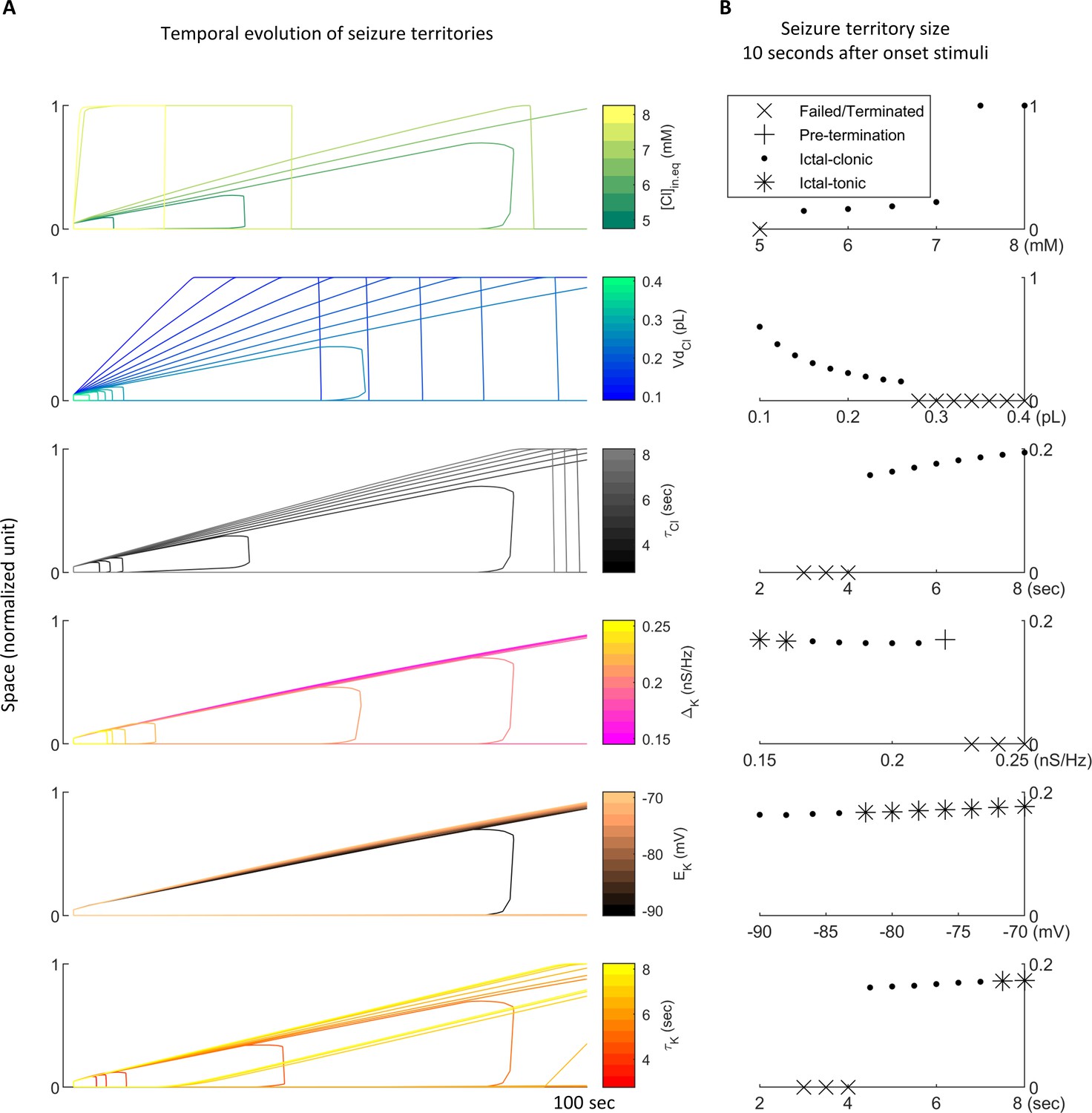
Targeted parameter search of seizure territory expansion.
(A) Expansion of seizure territories in space-time diagrams. Model parameters are derived from Table 1, with colors correspond with modifications indicated in the color bars. All seizures are provoked by 200 pA current injection during 2–5 s at location 0 to 0.05. Notice parameters which control inhibition robustness (chloride dynamics, the upper three panels) have more prominent effects on seizure expansion speed. (B) Seizure expansion speed quantified by measuring seizure territory size 10 seconds after the onset stimuli. Each subpanel aligns with the correspondent subpanel in panel A. Upper 3 subpanels: compromised inhibition robustness due to high , small , and slow is associated with fast seizure propagation. Lower 3 subpanels: strong adaptation currents due to high , low , and fast speed up stage transitions of seizure evolution.
Figure 2—figure supplement 4
Stages of focal seizure evolution in a generalized model of exhaustible inhibition.
(A) Figure conventions adopted from Figure 2A. Parameters are adopted from Table 1 with the following adjustments: =0.125 nS/Hz; =7 seconds; =15 nS; =125 nS; =-60 mV. Green box: deterministic external current input: =200 pA. (B) One-second temporal zoom-in of the ictal clonic stage, marked in Panel A. Figure convention adopted from Figure 2B. (C) Snapshots of inhibition effectiveness (z) and sAHP conductance (). Timing of the snapshots are marked in Panel A. Notice that inhibition collapses ahead of upregulation of the sAHP conductance.
Figure 3
Pre-termination stage shows ‘slowing-down’ dynamics.
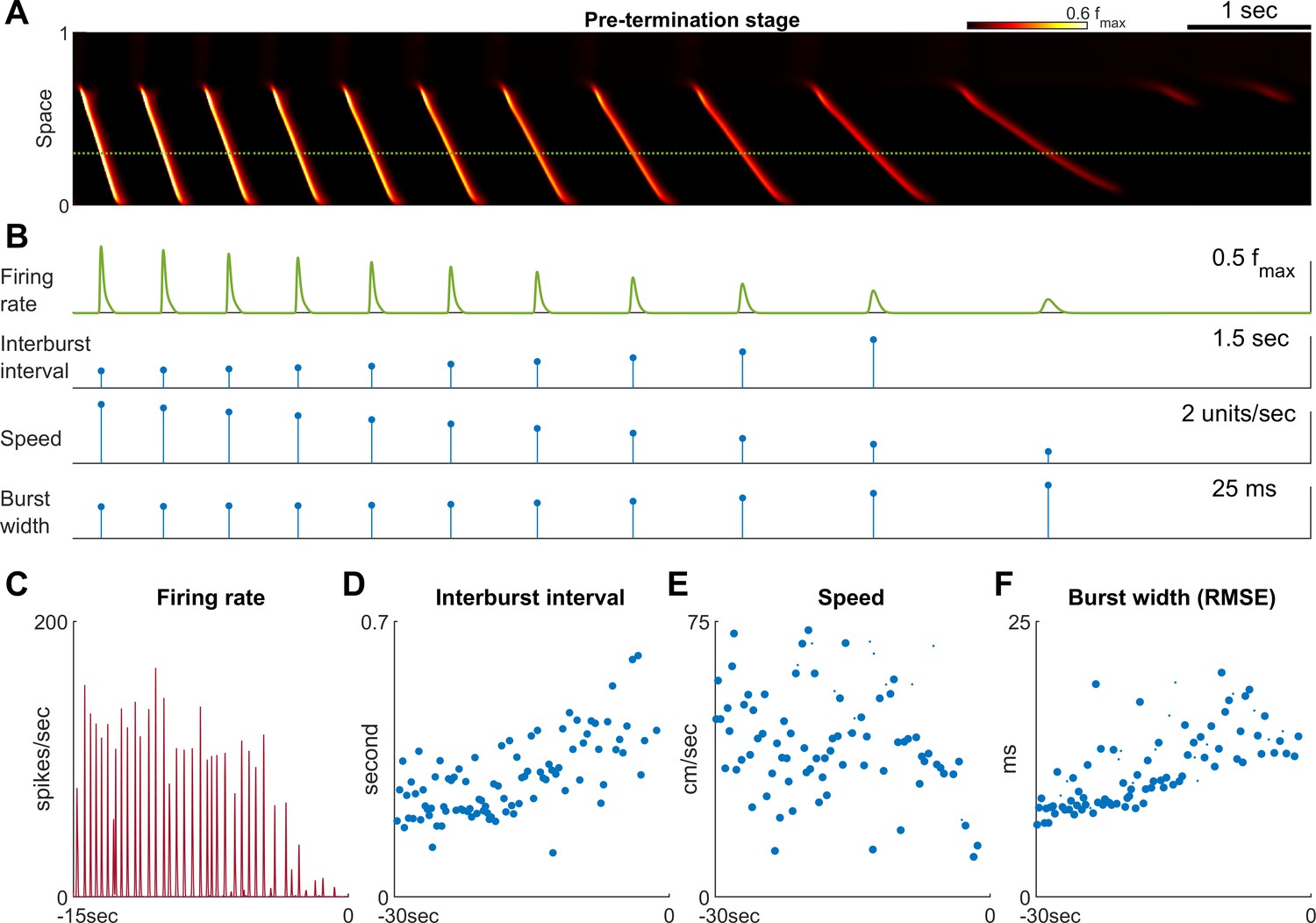
(A) Model seizure, pre-termination stage, zoomed-in from Figure 2A. The horizontal axis is shared with Panel B. The local neuronal population dynamics marked by the dotted green line is further shown in Panel B. Notice that in a space-time diagram a traveling wave is a slant band whose slope is its traveling velocity. (B) Quantification of the local neuronal population dynamics marked by the dotted green line in Panel A. Peak firing rate decreases, interburst intervals prolong, traveling wave speed decreases, and burst width decreases as the model seizure approaches termination. Neural activity within a region of 0.05 normalized distance centered at the dotted green line is used to calculate traveling wave speed. Burst width is calculated by first treating during each burst (100 ms temporal window) as a distribution and then estimate its standard deviation. (C–F) Patient B shows similar trends of neural dynamics at pre-termination stage. Peak firing rate decreased (C) interburst interval increased (D), traveling wave speed decreased (E), and burst width increased (F). Spearman’s correlation coefficients: -0.62 (n=35, p<0.001), 0.64 (n=93, p<0.001), -0.34 (n=93, p=0.002), 0.78 (n = 93, p<0.001) for C-F respectively.
Figure 4 with 1 supplement
Subtypes of seizure onset pattern can arise from different distributions of recurrent inhibition.
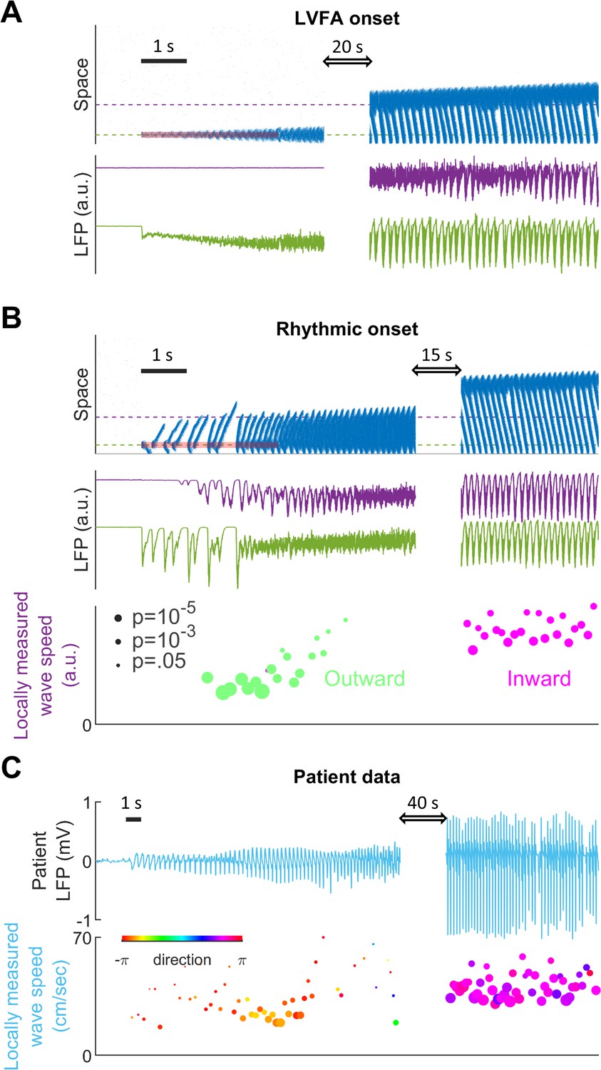
(A) LVFA onset (=-60mV, =1/6, =1.5 mV). Upper subpanel: raster plot of the spiking model. Horizontal axis: time. Vertical axis: space. Shaded red zone: =80 pA. Green and purple dashed lines indicate where the simulated LFPs, shown in the lower subpanel, are read out. LVFA is associated with large DC shift of the LFP, corresponding to seizure onset and ictal wavefront invasion. Periodic LFP discharges emerge after ictal wavefront passage (blank region: 20-second simulation result skipped for visualization). (B) Rhythmic onset (=-60mV, =1/2, =1.5 mV). Upper and middle subpanels inherit the conventions of panel A. At seizure onset, waves are generated and travel outwardly (shaded red area, =80pA). They are associated with rhythmic LFP discharges and precede the fast activity. Inward traveling waves emerge after wavefront establishment (after the blank interval). Lower subpanel: comparison of speeds between outward and inward traveling waves. Traveling wave speeds are measured locally at the location indicated by the purple dashed line, with each dot’s X-coordinate as the time of local firing rate max. Dot size corresponds to F-test p-value (significance level: 0.001) and color represents the direction of propagation. Outward waves (n=34) travel at a significantly lower speed than inward waves (n=23) (U-test, p<0.001). (C) Rhythmic seizure onset recorded from Patient B. Upper subpanel: averaged LFP recorded from the microelectrode array. Lower subpanel: traveling wave direction (dot color) and speed (Y-coordinates), estimated according to the spatiotemporal distribution of multiunit spikes. The seizure started with periodic LFP discharges before fast activity emerged. As the seizure evolved, traveling wave direction switched (dot color: orange to purple) and the speed increased (U-test p<0.001, n = 67 versus 49), analogous to the outward-to-inward switch predicted in Panel B.
Figure 4—figure supplement 1
Local environment determines seizure onset, propagation and termination patterns.
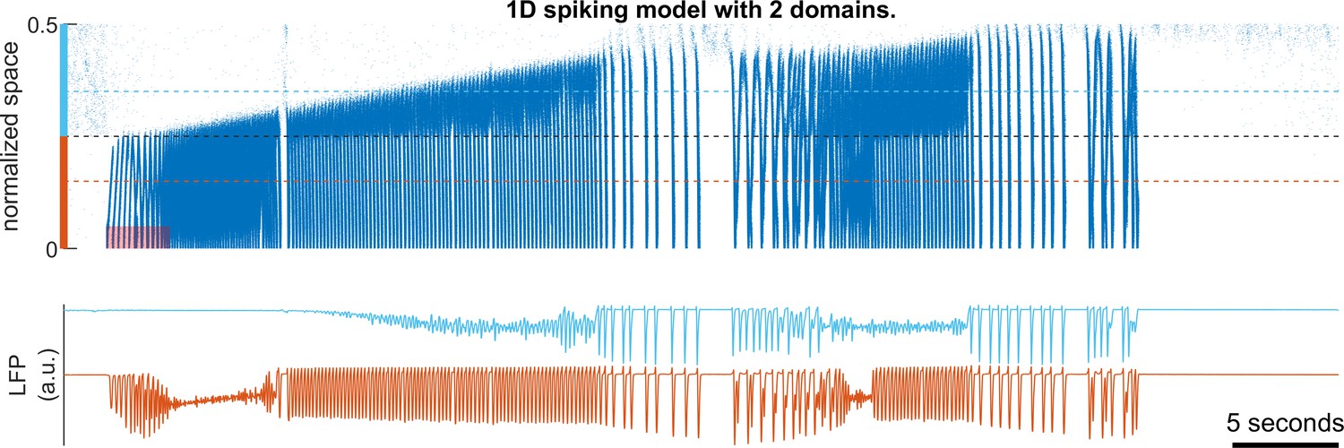
Upper panel: raster plot of a model seizure simulated in a spiking network with two domains (light blue and orange). The upper part of the space (light blue) is configured as Figure 2-figure supplement 1 (=1/6), whereas the lower part (orange) is configured as Figure 4B (=1/2). The gray dashed line indicates the boundary between the two domains. The light blue and orange dashed lines indicate where the simulated LFPs, shown in the lower subpanel, are calculated. The shaded red area: =80 pA. Outward traveling waves with rhythmic LFP discharges can be seen at the lower domain; whereas LFP simulated in the upper domain shows LVFA soon after seizure onset. The seizure approaches termination two times but fails the first time. Notice the characteristic slowing pre-termination dynamics is associated with inward traveling waves arising from the upper domain.
Figure 5
Connectivity induced by spike-timing dependent plasticity may promote emergence of seizure foci.
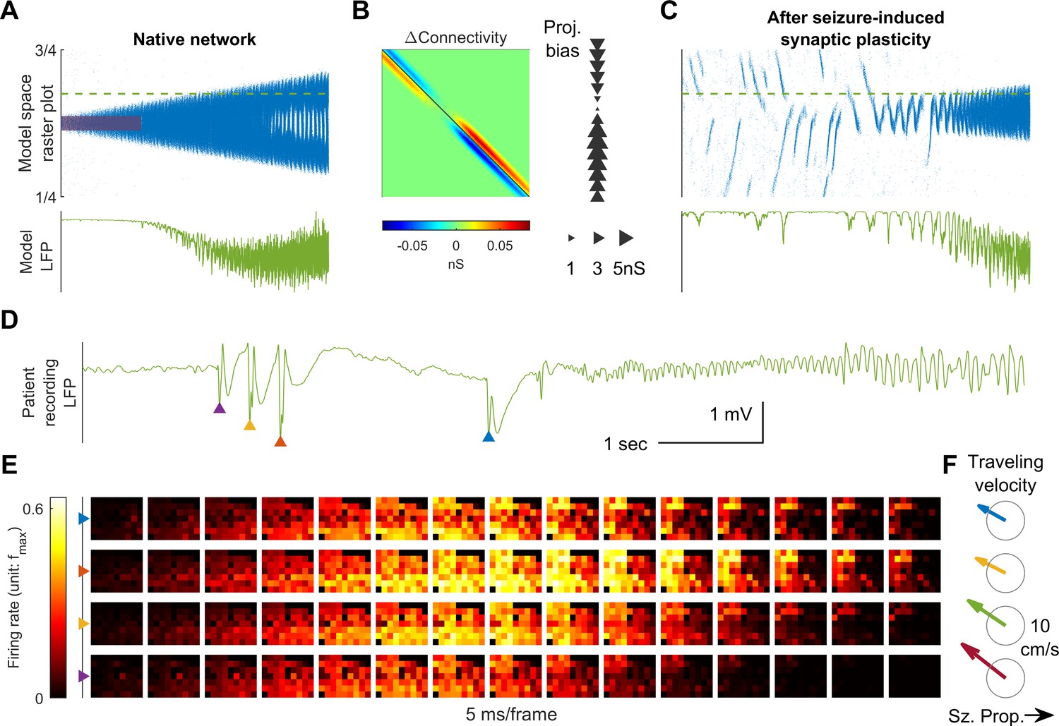
(A) Raster plot of a provoked model seizure with LVFA onset pattern. Figure conventions are inherited from Figure 4A. Red shaded area indicates the epileptogenic input =200 pA for 3 seconds). Stochastic background input: =20 pA, =0.1, =15 ms. The vertical axis is normalized spatial scale and aligned with Panel B and C. The green dashed line indicates where the simulated LFP, shown in the lower subpanel, is calculated. (=0.05 nS, =1.5 mV) (B) Changes in recurrent excitatory connectivity strength, , induced by STDP after the provoked model seizure (rows correspond to postsynaptic labels, columns to presynaptic). Left subpanel: the matrix. Right subpanel: neuronal projection bias calculated from the matrix (see Materials and methods). The location, size, and direction of the triangles represent the position of the neuron, magnitude and direction of the neuron's projection bias respectively. (C) A spontaneous seizure after seizure-induced synaptic plasticity (=0 pA). Several large amplitude LFP discharges, shown in the lower subpanel, precede the seizure onset. These LFP discharges are generated by the centripetal traveling waves seen in the raster plot. (D) LFP discharges recorded immediately before Patient A’s seizure onset. Discharges are marked by triangles of different colors. Evolution of the associated multiunit firing pattern is shown in Panel E. (E) Multiunit firings constitute traveling waves (10 ms kernel) before LVFA seizure onset. Note that the right half of the array detected multiunit firings earlier than the left half, which is opposite to the expansion direction of the ictal core (left to right). (F) Estimated traveling wave direction and speed. Gray circle: 10 cm/sec.
Figure 6 with 3 supplements
Consistent inward traveling wave direction can emerge from white noise.
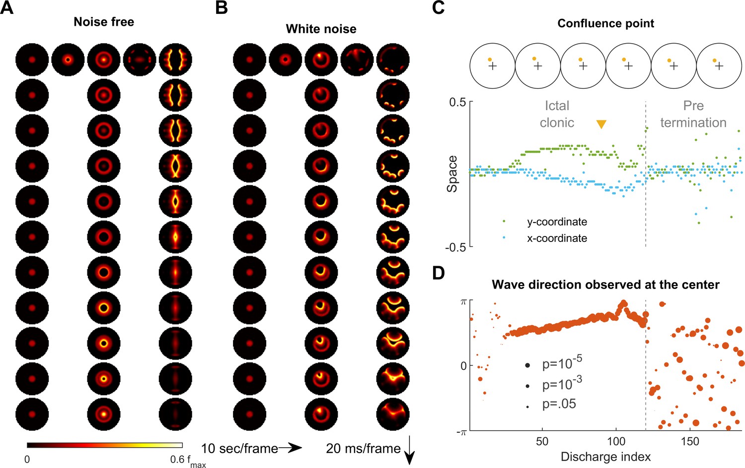
(A) Simulation results of a spatially bounded, two-dimensional rate model under a noise free condition. The epileptogenic stimulus was provided at the center of the round field (=200 pA, 3 second, stimulation radius = 0.05). Seizure territory slowly expands (the top row, left to right, 10 seconds per frame) and evolves in stages. The 1st column shows the tonic stage during which the firing rate within the seizure territory stays largely constant (20 ms per frame vertically). The 2nd and 3rd columns show the clonic and pre-termination stages, respectively. Because the neural sheet is symmetric and noise-free, all inward traveling waves meet exactly at the center. (B) Simulation protocol as in panel A but with spatiotemporally white noise with diffusion coefficient 200 pA2/ms is injected uniformly over the whole neural sheet. The confluence point of inward traveling waves during the clonic stage deviates from the center (middle column). Complex, asymmetric traveling wave generation is observed during the pre-termination stage (right column). (C) Locations of confluence points, quantified from Panel B. The upper row: confluence point locations of 6 consecutive inward traveling waves (marked in yellow). The lower subpanel: evolution of the confluence point locations. During the clonic stage (n=120), confluence points significantly deviate from the center (signed-rank test for both and coordinates, p <0.001) and drift slowly (auto-correlation coefficients: =0.82, =0.83; both p < 0.001.). (D) Traveling wave direction estimated at the center (radius = 0.05). White noise generates a consistent traveling wave direction during the clonic stage once the confluence point drifts away from the center. Circular auto-correlation during the ictal clonic stage: 0.97, p<0.001, n = 120. However, traveling wave direction becomes more variable during the pre-termination stage: =0.09, p=0.5, n = 65.
Figure 6—figure supplement 1
Increasing traveling wave direction variability as Patient B’s seizure approached termination.
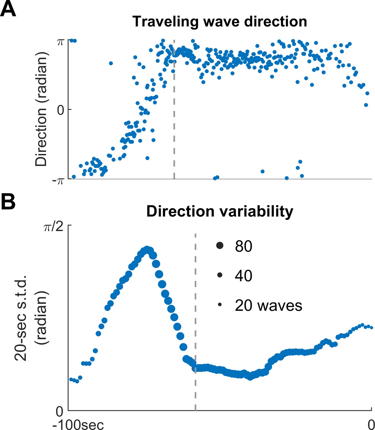
(A) Directions of Patient B’s ictal traveling waves before seizure termination (the same ones as shown in Figure 3). Horizontal axis: time. The axis is shared with Panel B. (B) Evolution of traveling direction variability estimated by a 20 s moving window, plotted every 1 s, quantified by circular standard deviation. Traveling wave direction variability increases as the seizure approaches termination (Spearman’s correlation coefficient: 0.95, p<0.001, n = 50).
Figure 6—video 1
Full evolution of the model seizure shown in Figure 6A.
Figure 6—video 2
Full evolution of the model seizure shown in Figure 6B.
Figure 7 with 1 supplement
Emergence of spiral waves, status epilepticus, and seizure termination induced by globally synchronizing inputs.
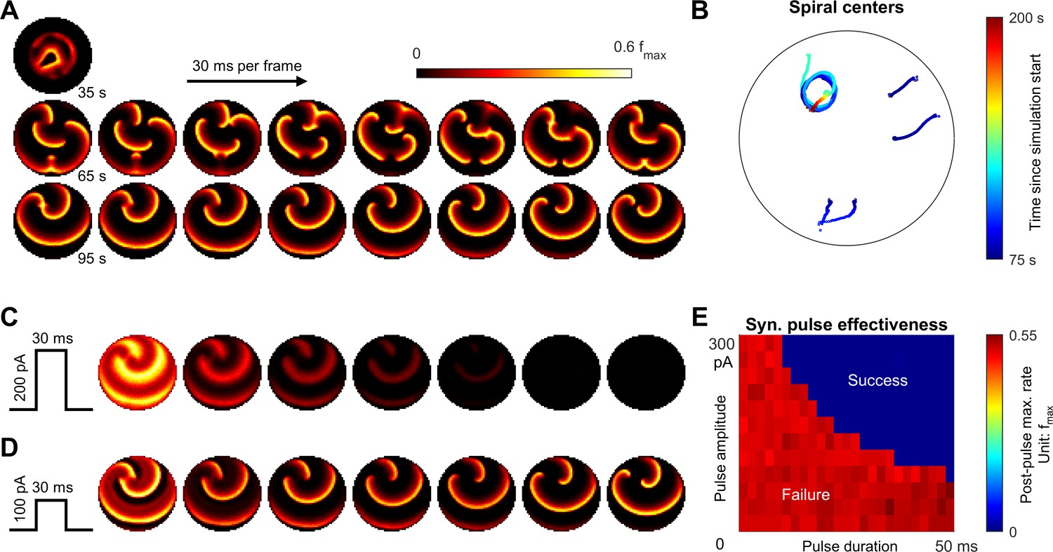
(A) Spiral wave formation. Model parameters and figure conventions are inherited from Figure 6B. The top snapshot shows the ical-clonic stage, then several spiral waves emerged after ictal wavefront annihilation (the upper row of snapshots). Spiral waves demonstrate complex interactions. Some spiral centers survived and persisted indefinitely (the lower row). (B) Movement of spiral wave centers, quantified from Panel A. In this simulation, one spiral wave eventually dominated the whole field and never terminated. (C) A globally synchronizing pulse with adequate amplitude and duration (=200pA, 30 ms) forced the spiral-wave seizure to terminate. The pulse was given at the time of the left lower sub-panel in Panel A. Each subpanel is aligned with the lower row of Panel A for comparison. (D) As C, but with inadequate amplitude (=100pA) to terminate the seizure. (E) Results of the pulse synchronization study. Color code: maximal firing rate across the neural network within 3 s after the pulse.
Figure 7—video 1
Full evolution of the model seizure shown in Figure 7.
Author response image 1

You can see several neighborhoods of depolarization caused by recently spiked neurons, which can be identified by their hyperpolarized membrane potentials (remember the spiking rule is: V ← V-20mV).
Tables
Table 1
Rate model parameters.
Neurons are modelled analogous to neocortical pyramidal neurons in terms of cell capacitance, leak conductance, and membrane time constant (Tripathy et al., 2014). Maximal synaptic conductances during seizures have been reported in the range of a few hundreds of nS (Neckelmann et al., 2000). Chloride clearance (Deisz et al., 2011), buffer (Marchetti, 2005), and seizure-induced sAHP conductance (Alger and Nicoll, 1980) are modeled according to the reported ranges. Spatially non-localized recurrent projections () are considered in this study (Liou et al., 2018). All rate models are based on this standard parameter set. Any further parameter adjustment is reported in figure legends.
| Parameters | unit | |
|---|---|---|
| 100 | pF | |
| 4 | nS | |
| 100 | nS | |
| 300 | nS | |
| -58 | mV | |
| 0 | mV | |
| -90 | mV | |
| 200 | Hz | |
| 2.5 | mV | |
| 15 | ms | |
| 15 | ms | |
| 100 | ms | |
| -45 | mV | |
| 0.3 | mV/Hz | |
| 5 | second | |
| 0.24 | pL | |
| 6 | mM | |
| 110 | mM | |
| 5 | second | |
| 0.2 | nS/Hz | |
| 0.02 | Normalized spatial scale | |
| 0.03 | Normalized spatial scale | |
| 1/6 |
Table 2
Spiking model parameters.
Parameters are chosen as described in the legend of Table 1. Time constant of spike timing dependent plasticity is chosen according to previously reported data (Bi and Poo, 1998; Song et al., 2000).
| Parameters | unit | |
|---|---|---|
| 100 | pF | |
| 4 | nS | |
| 100 | nS | |
| 300 | nS | |
| -57 | mV | |
| 0 | mV | |
| -90 | mV | |
| 2 | Hz | |
| 2.5 | mV | |
| 5 | ms | |
| 15 | ms | |
| 15 | ms | |
| 100 | mV | |
| -55 | mV | |
| 2.5 | mV | |
| 5 | Second | |
| 0.24 | pL | |
| 6 | mM | |
| 110 | mM | |
| 5 | Second | |
| 0.04 | nS | |
| 0.02 | Normalized spatial scale | |
| 0.03 | Normalized spatial scale | |
| 1/6 | ||
| 15 | ms |
Additional files
-
Source data 1
Patient A Seizure.
- https://cdn.elifesciences.org/articles/50927/elife-50927-data1-v1.mat
-
Source data 2
Patient B Seizure 1.
- https://cdn.elifesciences.org/articles/50927/elife-50927-data2-v1.mat
-
Source data 3
Patient B Seizure 2.
- https://cdn.elifesciences.org/articles/50927/elife-50927-data3-v1.mat
-
Source data 4
Patient B Seizure 3.
- https://cdn.elifesciences.org/articles/50927/elife-50927-data4-v1.mat
-
Transparent reporting form
- https://cdn.elifesciences.org/articles/50927/elife-50927-transrepform-v1.pdf
Download links
A two-part list of links to download the article, or parts of the article, in various formats.
Downloads (link to download the article as PDF)
Open citations (links to open the citations from this article in various online reference manager services)
Cite this article (links to download the citations from this article in formats compatible with various reference manager tools)
A model for focal seizure onset, propagation, evolution, and progression
eLife 9:e50927.
https://doi.org/10.7554/eLife.50927


