Identifying prostate cancer and its clinical risk in asymptomatic men using machine learning of high dimensional peripheral blood flow cytometric natural killer cell subset phenotyping data
- John van Geest Cancer Research Centre, School of Science and Technology, Nottingham Trent University, United Kingdom
- Department of Computer Science, Loughborough University, United Kingdom
- Centre for Health, Ageing and Understanding Disease (CHAUD), School of Science and Technology, Nottingham Trent University, United Kingdom
- Department of Urology, University Hospitals of Leicester NHS Trust, United Kingdom
Figures
Figure 1
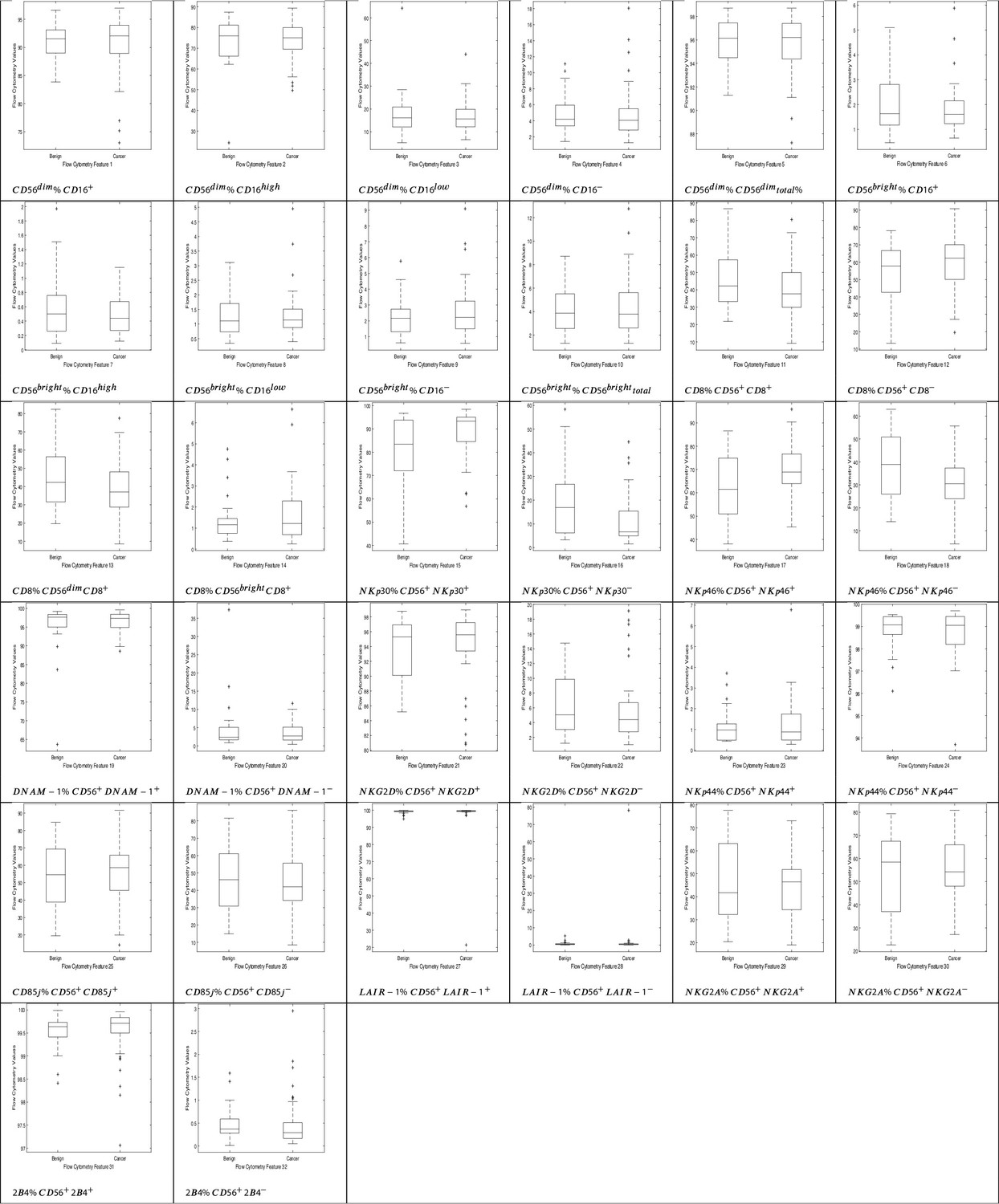
NK cell phenotypic features in men with benign prostate disease and patients with prostate cancer.
Boxplots represent the flow cytometry values of each feature for patients with benign disease and with prostate cancer.
Figure 2
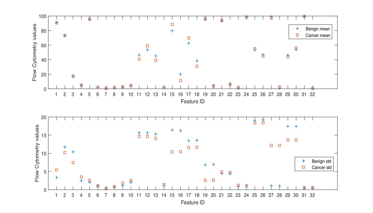
Mean and standard deviation values of flow cytometry features.
Figure 3
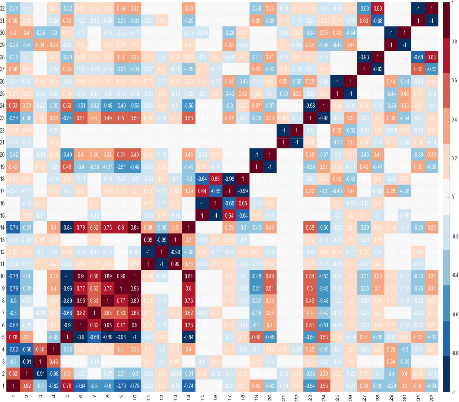
Correlations between features.
Figure 4
PSA values by group.
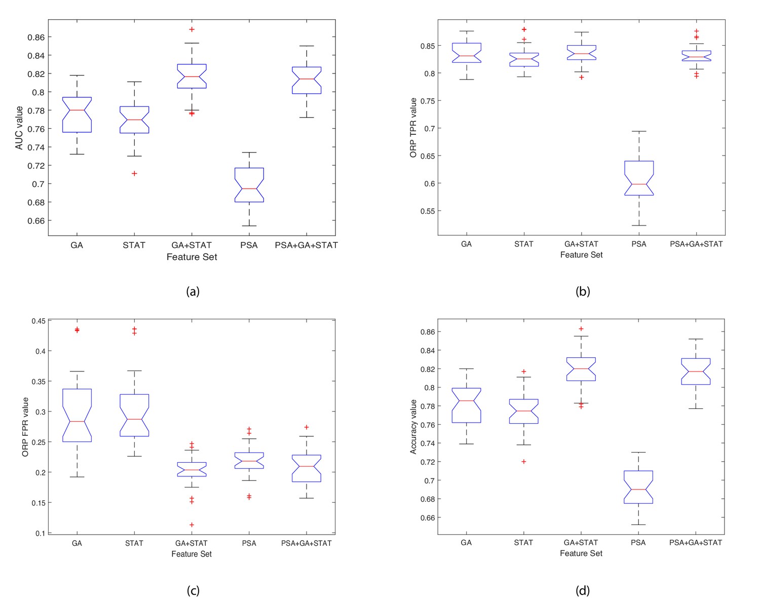
Figure 5

Boxplots illustrating the performance of the proposed model using various feature sets.
(a) Average AUC values, (b) Average Optimal ROC points (TPRs), (c) Average Optimal ROC points (FPRs), (d) Average Accuracy values. Each box plot contains 30 points, where each point is the average performance evaluation value (i.e. AUC, ORP TPR, ORP FPR, Accuracy) from one 10-fold run using the various feature sets.
Figure 6
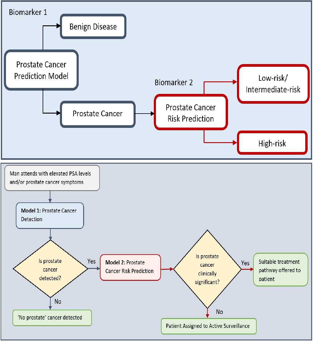
Flow charts illustrating the process to detect the presence and risk of prostate cancer and patient outcomes.
Model 1: Distinguishes between men with benign prostate disease and prostate cancer; Model 2: predicts risk (in terms of clinical significance) in men identified as having prostate cancer in Stage 1. Note that Model 1 can detect prostate cancer in men with PSA < 20 ng ml-1.
Figure 7
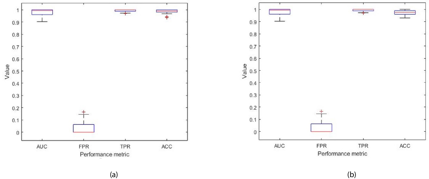
Each box plot contains 30 points, where each point is the average performance evaluation value (i.e. AUC, FPR, TPR, Accuracy (ACC)) from one 10-fold run during (a) k-fold validation results, and (b) independent testing results (i.e. using 10 patient records).
Figure 8
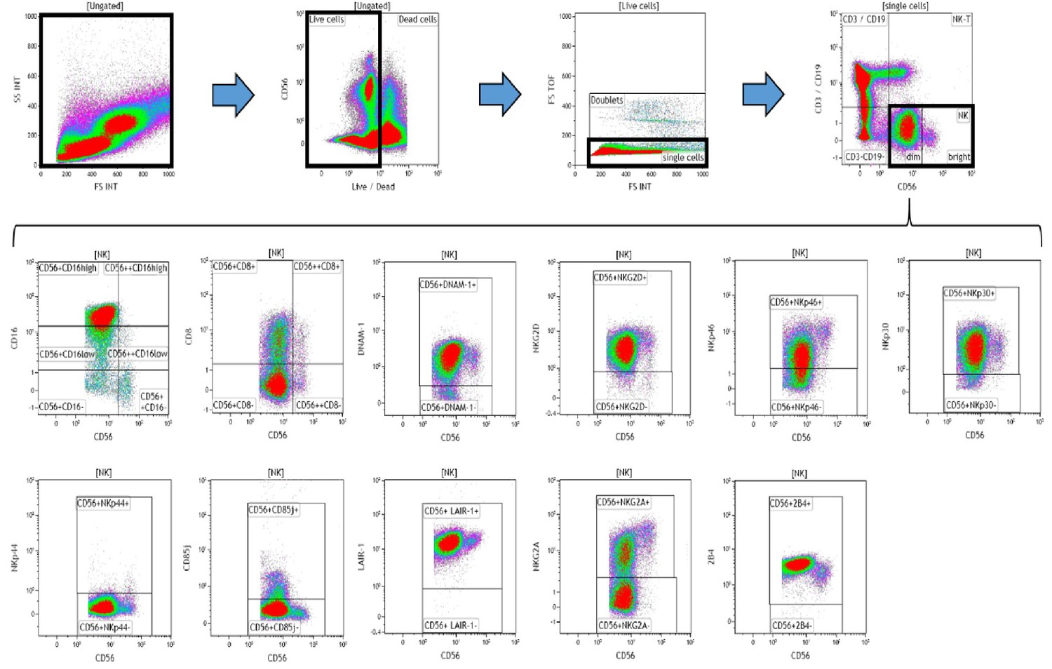
Representative gating strategy for analyzing the expression of activating and inhibitory receptors on peripheral blood natural killer (NK) cells.
Using density plots, the NK cell phenotypic profiles were determined by first gating on ‘live cells’ in the forward scatter (FSc) linear vs side scatter (SSc) linear density plot and then gating on single cells (determined by FSc Linear vs FS time of flight). The expression of activating and inhibitory receptors was determined by gating on cells using fluorescence minus one (FMO) controls. The expression of each NK cell receptor was measured using the ‘Logical’ setting.
Figure 9
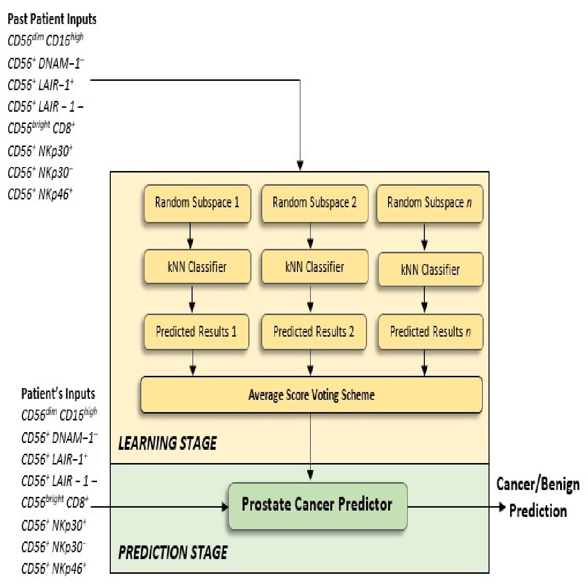
Proposed Ensemble Subspace kNN model.
Ensembles combine predictions from different models to generate a final prediction. Because Ensemble approaches combine baseline predictions, they perform at least as well as the best baseline model.
Tables
Table 1
Descriptive statistics of the dataset.
| Min. | Max. | Mean | Std. | IQR | Range | Diff. | ||||||||
|---|---|---|---|---|---|---|---|---|---|---|---|---|---|---|
| Beni. | Canc. | Beni. | Canc. | Beni. | Canc. | Beni. | Canc. | Beni. | Canc. | Beni. | Canc. | |||
| PSA | 4.70 | 4.70 | 19.00 | 19.00 | 8.26 | 8.34 | 3.31 | 3.28 | 3.30 | 4.08 | 14.30 | 14.30 | −0.08 | |
| % | ||||||||||||||
| 1 | 83.85 | 73.04 | 96.61 | 96.98 | 90.98 | 90.64 | 3.35 | 5.46 | 4.13 | 5.02 | 12.76 | 23.94 | 0.34 | |
| 2 | 24.38 | 49.66 | 87.46 | 89.33 | 72.88 | 73.32 | 11.74 | 10.22 | 15.00 | 10.45 | 63.08 | 39.67 | −0.44 | |
| 3 | 5.17 | 6.57 | 64.22 | 44.00 | 17.74 | 16.84 | 10.40 | 7.45 | 8.76 | 7.66 | 59.05 | 37.43 | 0.90 | |
| 4 | 1.41 | 1.25 | 11.11 | 18.06 | 4.83 | 4.89 | 2.45 | 3.48 | 2.58 | 2.68 | 9.70 | 16.81 | −0.06 | |
| 5 | 91.29 | 87.24 | 98.70 | 98.70 | 95.81 | 95.53 | 2.02 | 2.58 | 2.96 | 3.02 | 7.41 | 11.46 | 0.28 | |
| % | ||||||||||||||
| 6 | 0.46 | 0.65 | 5.10 | 5.88 | 1.91 | 1.83 | 1.06 | 1.04 | 1.64 | 0.92 | 4.64 | 5.23 | 0.08 | |
| 7 | 0.09 | 0.12 | 1.97 | 1.15 | 0.60 | 0.47 | 0.44 | 0.25 | 0.50 | 0.40 | 1.88 | 1.03 | 0.13 | |
| 8 | 0.34 | 0.40 | 3.11 | 4.95 | 1.27 | 1.35 | 0.72 | 0.86 | 0.97 | 0.63 | 2.77 | 4.55 | −0.07 | |
| 9 | 0.61 | 0.58 | 5.78 | 9.09 | 2.28 | 2.64 | 1.14 | 1.82 | 1.42 | 1.75 | 5.17 | 8.51 | −0.36 | |
| 10 | 1.30 | 1.30 | 8.71 | 12.76 | 4.19 | 4.47 | 2.02 | 2.58 | 2.95 | 3.01 | 7.41 | 11.46 | −0.28 | |
| % | ||||||||||||||
| 11 | 21.88 | 9.20 | 86.70 | 80.47 | 46.43 | 40.71 | 15.64 | 14.66 | 24.03 | 20.05 | 64.82 | 71.27 | 5.72 | |
| 12 | 13.30 | 19.53 | 78.12 | 90.80 | 53.57 | 59.29 | 15.64 | 14.66 | 24.03 | 20.05 | 64.82 | 71.27 | −5.72 | |
| 13 | 19.63 | 8.60 | 82.38 | 77.47 | 45.18 | 39.11 | 15.31 | 14.10 | 24.72 | 19.36 | 62.75 | 68.87 | 6.07 | |
| 14 | 0.37 | 0.25 | 4.75 | 6.64 | 1.41 | 1.70 | 1.07 | 1.41 | 0.70 | 1.60 | 4.38 | 6.39 | −0.29 | |
| NKp30 % | ||||||||||||||
| 15 | 40.69 | 56.80 | 96.74 | 98.43 | 79.78 | 88.56 | 16.42 | 10.41 | 21.80 | 10.44 | 56.05 | 41.63 | −8.78 | |
| 16 | 3.26 | 1.57 | 58.34 | 44.59 | 20.05 | 11.43 | 16.22 | 10.46 | 20.54 | 10.49 | 55.08 | 43.02 | 8.61 | |
| NKp46 % | ||||||||||||||
| 17 | 38.11 | 45.37 | 86.52 | 95.82 | 62.65 | 69.82 | 13.49 | 11.58 | 23.90 | 12.71 | 48.41 | 50.45 | −7.18 | |
| 18 | 14.02 | 4.32 | 62.97 | 55.68 | 38.40 | 30.87 | 13.58 | 11.64 | 24.89 | 13.44 | 48.95 | 51.36 | 7.53 | |
| DNAM-1 % | ||||||||||||||
| 19 | 63.69 | 88.56 | 99.18 | 99.60 | 95.35 | 96.46 | 6.81 | 2.59 | 3.37 | 3.49 | 35.49 | 11.04 | −1.11 | |
| 20 | 0.86 | 0.42 | 37.29 | 11.66 | 4.74 | 3.59 | 6.96 | 2.61 | 3.45 | 3.54 | 36.43 | 11.24 | 1.14 | |
| NKG2D % | ||||||||||||||
| 21 | 85.17 | 80.79 | 98.77 | 98.96 | 93.49 | 94.07 | 4.45 | 4.87 | 6.81 | 3.83 | 13.60 | 18.17 | −0.58 | |
| 22 | 1.22 | 1.03 | 14.76 | 19.12 | 6.44 | 5.84 | 4.36 | 4.76 | 6.80 | 3.96 | 13.54 | 18.09 | 0.60 | |
| PSA | 4.70 | 4.70 | 19.00 | 19.00 | 8.26 | 8.34 | 3.31 | 3.28 | 3.30 | 4.08 | 14.30 | 14.30 | −0.08 | |
| NKp44 % | ||||||||||||||
| 23 | 0.43 | 0.28 | 3.71 | 6.77 | 1.16 | 1.34 | 0.82 | 1.20 | 0.78 | 1.25 | 3.28 | 6.49 | −0.18 | |
| 24 | 96.10 | 93.70 | 99.53 | 99.70 | 98.82 | 98.64 | 0.83 | 1.13 | 0.80 | 1.25 | 3.43 | 6.00 | 0.18 | |
| CD85j % | ||||||||||||||
| 25 | 19.53 | 14.21 | 84.73 | 91.59 | 53.37 | 55.10 | 19.04 | 18.34 | 30.49 | 20.23 | 65.20 | 77.38 | −1.74 | |
| 26 | 14.93 | 8.50 | 81.54 | 86.08 | 46.94 | 45.24 | 19.21 | 18.43 | 30.28 | 21.48 | 66.61 | 77.58 | 1.69 | |
| LAIR-1 % | ||||||||||||||
| 27 | 94.97 | 21.43 | 99.90 | 99.89 | 99.07 | 97.47 | 1.07 | 12.19 | 0.49 | 0.47 | 4.93 | 78.46 | 1.60 | |
| 28 | 0.02 | 0.05 | 5.24 | 78.20 | 0.76 | 2.40 | 1.02 | 12.15 | 0.42 | 0.43 | 5.22 | 78.15 | −1.65 | |
| NKG2A % | ||||||||||||||
| 29 | 20.43 | 19.01 | 77.57 | 73.01 | 46.14 | 44.24 | 17.41 | 13.73 | 30.82 | 17.47 | 57.14 | 54.00 | 1.90 | |
| 30 | 22.62 | 27.11 | 79.40 | 80.85 | 54.01 | 55.99 | 17.39 | 13.67 | 30.48 | 17.90 | 56.78 | 53.74 | −1.98 | |
| 2B4 % | ||||||||||||||
| 31 | 98.41 | 97.06 | 99.99 | 99.96 | 99.53 | 99.50 | 0.39 | 0.59 | 0.32 | 0.33 | 1.58 | 2.90 | 0.02 | |
| 32 | 0.01 | 0.05 | 1.59 | 2.95 | 0.48 | 0.50 | 0.39 | 0.59 | 0.31 | 0.34 | 1.58 | 2.90 | −0.02 | |
-
Min. is the minimum value, Max. is maximum value, Mean is the mean or average value, and Std. is Standard Deviation. Range is the difference between the minimum and maximum values. The Interquartile range (IQR) is a measure of data variability and was derived by computing the distance between the Upper Quartile (i.e. top) and Lower Quartile (i.e. bottom) of the boxes illustrated in Figure 1. Difference is computed as diff = mean(Benign)-mean(Cancer).
Table 2
Tests of normality results.
| Tests of normality | ||||||||
|---|---|---|---|---|---|---|---|---|
| NK cell values | Kolmogorov-Smirnova | Shapiro-Wilk | ||||||
| Statistic | df | Sig. | Statistic | df | Sig. | |||
| 1 | 0.15 | 71.00 | 0.00 | 0.85 | 71.00 | 0.00 | ||
| 2 | 0.11 | 71.00 | 0.03 | 0.89 | 71.00 | 0.00 | ||
| 3 | 0.17 | 71.00 | 0.00 | 0.79 | 71.00 | 0.00 | ||
| 4 | 0.19 | 71.00 | 0.00 | 0.82 | 71.00 | 0.00 | ||
| 5 | 0.15 | 71.00 | 0.00 | 0.91 | 71.00 | 0.00 | ||
| 6 | 0.13 | 71.00 | 0.00 | 0.88 | 71.00 | 0.00 | ||
| 7 | 0.15 | 71.00 | 0.00 | 0.87 | 71.00 | 0.00 | ||
| 8 | 0.14 | 71.00 | 0.00 | 0.85 | 71.00 | 0.00 | ||
| 9 | 0.16 | 71.00 | 0.00 | 0.86 | 71.00 | 0.00 | ||
| 10 | 0.15 | 71.00 | 0.00 | 0.91 | 71.00 | 0.00 | ||
| 11 | 0.10 | 71.00 | 0.06 | 0.98 | 71.00 | 0.17 | ||
| 12 | 0.10 | 71.00 | 0.06 | 0.98 | 71.00 | 0.17 | ||
| 13 | 0.09 | 71.00 | 0.20* | 0.98 | 71.00 | 0.24 | ||
| 14 | 0.19 | 71.00 | 0.00 | 0.82 | 71.00 | 0.00 | ||
| 15 | 0.21 | 71.00 | 0.00 | 0.81 | 71.00 | 0.00 | ||
| 16 | 0.21 | 71.00 | 0.00 | 0.81 | 71.00 | 0.00 | ||
| 17 | 0.08 | 71.00 | 0.20* | 0.98 | 71.00 | 0.52 | ||
| 18 | 0.07 | 71.00 | 0.20* | 0.99 | 71.00 | 0.57 | ||
| 19 | 0.23 | 71.00 | 0.00 | 0.56 | 71.00 | 0.00 | ||
| 20 | 0.23 | 71.00 | 0.00 | 0.55 | 71.00 | 0.00 | ||
| 21 | 0.19 | 71.00 | 0.00 | 0.84 | 71.00 | 0.00 | ||
| 22 | 0.18 | 71.00 | 0.00 | 0.85 | 71.00 | 0.00 | ||
| 23 | 0.18 | 71.00 | 0.00 | 0.76 | 71.00 | 0.00 | ||
| 24 | 0.17 | 71.00 | 0.00 | 0.78 | 71.00 | 0.00 | ||
| 25 | 0.11 | 71.00 | 0.05 | 0.96 | 71.00 | 0.02 | ||
| 26 | 0.10 | 71.00 | 0.07 | 0.96 | 71.00 | 0.02 | ||
| 27 | 0.43 | 71.00 | 0.00 | 0.14 | 71.00 | 0.00 | ||
| 28 | 0.43 | 71.00 | 0.00 | 0.14 | 71.00 | 0.00 | ||
| 29 | 0.09 | 71.00 | 0.20* | 0.97 | 71.00 | 0.11 | ||
| 30 | 0.08 | 71.00 | 0.20* | 0.97 | 71.00 | 0.10 | ||
| 31 | 0.23 | 71.00 | 0.00 | 0.75 | 71.00 | 0.00 | ||
| 32 | 0.23 | 71.00 | 0.00 | 0.75 | 71.00 | 0.00 | ||
-
*. This is a lower bound of the true significance.
Those values in bold are of those features whose data is normally distributed.
-
If the , we can accept the null hypothesis, that there is no statistically significant difference between the data and the normal distribution, hence we can presume that the data of those features are normally distributed.
If the , we can reject the null hypothesis because there is a statistically significant difference between the data and the normal distribution, hence we can presume that the data of those features are not normally distributed.
Table 3
Results of the Kruskal-Wallis test.
| Chi-Sq.() | Asy. sig. p value | |||
|---|---|---|---|---|
| PSA | 0 | 0.949 | ||
| NK cells | ||||
| 1 | 0.001 | 0.981 | ||
| 2 | 0.069 | 0.793 | ||
| 3 | 0.555 | 0.456 | ||
| 4 | 0.033 | 0.857 | ||
| 5 | 0.063 | 0.802 | ||
| 6 | 0.836 | 0.361 | ||
| 7 | 0.201 | 0.654 | ||
| 8 | 0.106 | 0.744 | ||
| 9 | 0.030 | 0.861 | ||
| 10 | 2.415 | 0.120 | ||
| 11 | 2.415 | 0.120 | ||
| 12 | 2.849 | 0.091 | ||
| 13 | 0.417 | 0.518 | ||
| 14 | 7.230 | 0.007 | ||
| 15 | 7.106 | 0.008 | ||
| 16 | 4.638 | 0.031 | ||
| 17 | 5.179 | 0.023 | ||
| 18 | 0.001 | 0.981 | ||
| 19 | 0.001 | 0.972 | ||
| 20 | 0.293 | 0.588 | ||
| 21 | 0.325 | 0.568 | ||
| 22 | 0.033 | 0.857 | ||
| 23 | 0.072 | 0.789 | ||
| 24 | 0.049 | 0.825 | ||
| 25 | 0.072 | 0.789 | ||
| 26 | 2.135 | 0.144 | ||
| 27 | 1.343 | 0.247 | ||
| 28 | 0.060 | 0.807 | ||
| 29 | 0.072 | 0.789 | ||
| 30 | 0.879 | 0.348 | ||
| 31 | 0.890 | 0.346 | ||
| 32 | 0.890 | 0.346 | ||
Table 4
Results of the Genetic Algorithm when searching for the best subset of features.
| No. different comb | Comb. with highest freq. | Freq. of comb. | Relative freq. (%) | |
|---|---|---|---|---|
| 2 | 3 | 17,28 | 16 | 53.3 |
| 3 | 2 | 17,27,29 | 23 | 76.7 |
| 4 | 1 | 2,20,27,28 | 30 | 100.0 |
| 5 | 2 | 3,20,27,28,32 | 29 | 96.7 |
| 6 | 2 | 3,7,20,27,28,32 | 26 | 86.7 |
| 7 | 3 | 3,7,20,23,27,28,32 | 24 | 80.0 |
| 8 | 4 | 3,7,20,22,23,27,28,32 | 19 | 63.3 |
| 9 | 3 | 3,7,19,20,22,23,27,28,32 | 24 | 80.0 |
| 10 | 3 | 2,3,7,19,20,22,23,27,28,32 | 21 | 70.0 |
Table 5
Naming of the models includes the feature selection method (GA) combined with the proposed Ensemble Subspace kNN classifier.
Validation results are presented at k = 10 fold cross validation.
| Results of 10-fold cross validation over 30 runs | |||||||
|---|---|---|---|---|---|---|---|
| AUC | Orp fpr | Orp tpr | ACC | Mean std. | Rank | ||
| GA | Mean | 0.776 | 0.296 | 0.833 | 0.781 | 4 | |
| Std. | 0.024 | 0.065 | 0.026 | 0.023 | 0.035 | ||
| STAT | Mean | 0.769 | 0.303 | 0.828 | 0.774 | 5 | |
| Std. | 0.022 | 0.057 | 0.023 | 0.021 | 0.031 | ||
| GA+STAT | Mean | 0.818 | 0.201 | 0.836 | 0.821 | 1 | |
| Std. | 0.021 | 0.027 | 0.021 | 0.020 | 0.022 | ||
| PSA+GA+STAT | Mean | 0.812 | 0.208 | 0.832 | 0.815 | 2 | |
| Std. | 0.020 | 0.031 | 0.018 | 0.019 | 0.022 | ||
| PSA | Mean | 0.698 | 0.217 | 0.609 | 0.692 | 6 | |
| Std. | 0.022 | 0.025 | 0.043 | 0.020 | 0.028 | ||
| All features | Mean | 0.812 | 0.213 | 0.836 | 0.815 | 3 | |
| Std. | 0.022 | 0.035 | 0.021 | 0.021 | 0.025 | ||
Table 6
Comparing the performance of the proposed Ensemble Subspace kNN model against conventional machine learning models when using the GA+STAT feature set.
Results of 10-fold cross validation over 30 runs.
| Proposed ensemble subspace kNN (EkNN) model | ||||||
|---|---|---|---|---|---|---|
| (No. of learners (NL): 30; Subspace Dimension (SD): 16) | ||||||
| Parameters | AUC | ORP FPR | ORP TPR | ACC | ||
| NL: 30, SD:16 | Mean | 0.818 | 0.201 | 0.836 | 0.821 | |
| Std. | 0.021 | 0.027 | 0.021 | 0.020 | ||
| Simple kNN model (Distance: Euclidean) | ||||||
| AUC | ORP FPR | ORP TPR | ACC | Acc. Diff. | ||
| k | (EkNN vs. kNN) | |||||
| 2 | Mean | 0.768 | 0.241 | 0.730 | 0.751 | +0.070 |
| Std. | 0.119 | 0.160 | 0.393 | 0.128 | −0.108 | |
| 5 | Mean | 0.778 | 0.300 | 0.833 | 0.783 | +0.038 |
| Std. | 0.107 | 0.265 | 0.103 | 0.103 | −0.083 | |
| 10 | Mean | 0.753 | 0.371 | 0.845 | 0.758 | +0.063 |
| Std. | 0.137 | 0.350 | 0.120 | 0.131 | −0.111 | |
| Support Vector Machine models | ||||||
| AUC | ORP FPR | ORP TPR | ACC | Acc. Diff. | ||
| Kernel | (EkNN vs. SVM) | |||||
| Linear | Mean | 0.782 | 0.342 | 0.860 | 0.784 | +0.037 |
| Std. | 0.126 | 0.352 | 0.110 | 0.120 | −0.100 | |
| Gaussian | Mean. | 0.808 | 0.353 | 0.876 | 0.799 | +0.022 |
| Std. | 0.112 | 0.416 | 0.107 | 0.111 | −0.091 | |
| Naive Bayes model | ||||||
| AUC | ORP FPR | ORP TPR | ACC | Acc. Diff. | ||
| Predictor distributions | (EkNN vs. Naïve Bayes) | |||||
| Normal | Mean. | 0.695 | 0.132 | 0.455 | 0.662 | +0.159 |
| Std. | 0.169 | 0.163 | 0.493 | 0.181 | −0.161 | |
Table 7
Ad hoc test results.
| Ad hoc test | ||||||
|---|---|---|---|---|---|---|
| Group 1 | Group 2 | Ll 95% | Diff. betw.means | Ul 95% | P | |
| 1 | GA | STAT | −12.658 | 1.317 | 15.292 | 1.000 |
| 2 | GA | GA+STAT | −22.208 | −8.233 | 5.742 | 0.525 |
| 3 | GA | PSA | −4.992 | 8.983 | 22.958 | 0.344 |
| 4 | GA | PSA+GA+STAT | −20.792 | −6.817 | 7.158 | 1.000 |
| 5 | STAT | GA+STAT | −23.525 | −9.550 | 4.425 | 0.245 |
| 6 | STAT | PSA | −6.308 | 7.667 | 21.642 | 0.710 |
| 7 | STAT | PSA+GA+STAT | −22.108 | −8.133 | 5.842 | 0.555 |
| 8 | GA+STAT | PSA | 3.242 | 17.217 | 31.192 | 0.001 |
| 9 | GA+STAT | PSA+GA+STAT | −12.558 | 1.417 | 15.392 | 1.000 |
| 10 | PSA | PSA+GA+STAT | −29.775 | −15.800 | −1.825 | 0.002 |
-
The first two columns show the groups that are compared. The third and fifth columns show the lower and upper limits for 95% confidence intervals for the true mean difference. The fourth column shows the difference between the estimated group means. The sixth column contains the p-value for testing a hypothesis that the corresponding mean difference is equal to zero.
Table 8
Results of the best prediction models created during the 30 runs.
Validation results are presented at k = 10 fold cross validation.
| Best prediction model results | |||||
|---|---|---|---|---|---|
| AUC | Orp fpr | Orp tpr | Accuracy | Rank | |
| GA | 0.818 | 0.192 | 0.829 | 0.820 | 3 |
| GA+STAT | 0.853 | 0.157 | 0.862 | 0.855 | 1 |
| PSA | 0.734 | 0.218 | 0.685 | 0.730 | 5 |
| PSA+GA+STAT | 0.844 | 0.175 | 0.864 | 0.848 | 2 |
| STAT | 0.811 | 0.227 | 0.85 | 0.817 | 4 |
Key resources table
| Reagent type (species) or resource | Designation | Source or reference | Identifiers | Additional information |
|---|---|---|---|---|
| Biological Sample | Hyclone fetal bovine serum (FBS) | GE Healthcare Life Sciences | SV30180.03 | |
| Antibody | Monoclonal mouse IgG1 kappa anti human DNAM-1 (CD226) (clone 11A8); FITC | BioLegend | 338304 | 5 μl per tube / 106cells |
| Antibody | Monoclonal mouse IgG1 kappa anti human NKG2D (CD314) (clone 1D11); PE | eBioscience | 12-5878-42 | 5 μl per tube / 106cells |
| Antibody | Monoclonal mouse IgG1 kappa anti human CD56 (clone N901); ECD (PE-Texas Red) | Beckman Coulter | A82943 | 2.5 μl per tube / 106cells |
| Antibody | Monoclonal mouse IgG1 kappa anti human CD16 (clone 3G8); PerCP-Cy5.5 | BioLegend | 302028 | 5 μl per tube / 106cells |
| Antibody | Monoclonal mouse IgG1 kappa anti human NKp46 (CD335) (clone 9E2); PE-Cy7 | BioLegend | 331916 | 5 μl per tube / 106cells |
| Antibody | Monoclonal mouse IgG1 kappa anti human NKp30 (CD337) (clone P30-15); Alexa Fluor 647 | BioLegend | 325212 | 5 μl per tube / 106cells |
| Antibody | Monoclonal mouse IgG1 kappa anti human CD3 (clone UCHT1); Alexa Fluor 700 | BioLegend | 300424 | 2 μl per tube / 106cells |
| Antibody | Monoclonal mouse IgG1 kappa anti human CD19 (clone HIB19); Alexa Fluor 700 | BioLegend | 302226 | 1 μl per tube / 106cells |
| Antibody | Monoclonal mouse IgG1 kappa anti human CD8 (clone SK1); APC-Cy7 | BioLegend | 344714 | 2.5 μl per tube / 106cells |
| Antibody | Monoclonal mouse IgG2b anti human CD85j (ILT2) (clone GHI/75); FITC | Miltenyi Biotec | 130-098-437 | 10 μl per tube / 106cells |
| Antibody | Monoclonal mouse IgG1 kappa anti human LAIR-1 (CD305) (clone DX26); PE | BD Biosciences | 550811 | 20 μl per tube / 106cells |
| Antibody | Monoclonal mouse IgG2b anti human NKG2A (CD159a) (clone Z199); PE-Cy7(PC7) | Beckman Coulter | B10246 | 20 μl per tube / 106cells |
| Antibody | Monoclonal mouse IgG1 kappa anti human NKp44 (CD336) (clone P44-8); Alexa Fluor 647 | BioLegend | 325112 | 5 μl per tube / 106cells |
| Antibody | Monoclonal mouse IgG1 kappa anti human 2B4 (CD244.2) (clone C1.7); FITC | BioLegend | 329506 | 5 μl per tube / 106cells |
| Chemical Compound | LIVE/DEAD Fixable Violet Dead Stain | Thermo Fisher Scientific | L34955 | 1 μl in 1 μl |
| Chemical Compound | Novagen Benzonase Nuclease | Merck Millipore | 70664 | |
| Chemical Compound | CTL Wash Solution | Cellular Technology Limited | CTLW-010 | |
| Chemical Compound | Trypan Blue viability stain | Santa Cruz | sc-216028 | |
| Chemical Compound | Dimethyl sulfoxide (DMSO) | Santa Cruz | sc-202581 | |
| Chemical Compound | Calbiochem bovine serum albumin (BSA) | Merck Millipore | 2905-OP | |
| Chemical Compound | Sigma-Aldrich sodium azide | Merck Millipore | S8032 | |
| Chemical Compound | Sigma-Aldrich lithium heparin | Merck Millipore | H0878 | |
| Chemical Compound | Ficoll-Paque | GE Healthcare Life Sciences | 17-1440-03 | |
| Chemical Compound | Isoton II isotonic buffered saline solution | Beckman Coulter | 844 80 11 | |
| Chemical Compound | RPMI medium | Lonza | 12-167Q | |
| Chemical Compound | Phosphate Buffered Saline (PBS) | Lonza | 17-517Q | |
| Other | Leucosep tubes | Greiner Bio-One International | 227290 | |
| Software | Kaluza v1.3 | Beckman Coulter |
Table 9
Patient clinical features.
| Patient group | Gleason score | Number of patients | Age range (years) | PSA range (ng/ml) |
|---|---|---|---|---|
| Benign | Benign | 9 | 64-71 | 5.3–15 |
| Benign | HGPIN | 9 | 54–70 | 5.1–12 |
| Benign | Atypia | 10 | 50–76 | 4.7–19 |
| Benign | ASAP | 2 | 59–60 | 5.3–7.8 |
| Cancer | Gleason 6 | 16 | 55–80 | 4.7–11 |
| Cancer | Gleason 7 | 23 | 53–77 | 4.7–19 |
| Cancer | Gleason 9 | 2 | 65–75 | 6.3–18 |
Table 10
Dataset used for differentiating between patients with L/I and H cancer.
| Patient group | Count | % |
|---|---|---|
| L/I | 38 | 70.37 |
| H | 16 | 29.63 |
Table 11
Antibody panels for measuring the phenotype of Natural Killer cells.
| Antibody | Fluorochrome | Clone no. | Supplier |
|---|---|---|---|
| Panel 1 | |||
| DNAM-1 (CD226) | FITC | 11A8 | BioLegend |
| NKG2D (CD314) | PE | 1D11 | eBioscience |
| CD56 | ECD (PE-Texas Red) | N901 | Beckman Coulter |
| CD16 | PerCP-Cy5.5 | 3G8 | BioLegend |
| NKp46 (CD335) | PE-Cy7 | 9E2 | BioLegend |
| NKp30 (CD337) | Alexa Fluor 647 | P30-15 | BioLegend |
| CD3 | Alexa Fluor 700 | UCHT1 | BioLegend |
| CD19 | Alexa Fluor 700 | HIB19 | BioLegend |
| CD8 | APC-Cy7 | SK1 | BioLegend |
| Live/Dead | Dye (violet) | Thermo Fisher Scientific | |
| Panel 2 | |||
| CD85j (ILT2) | FITC | GHI/75 | Miltenyi Biotec |
| LAIR-1 (CD305) | PE | DX26 | BD Biosciences |
| CD56 | ECD (PE-Texas Red) | N901 | Beckman Coulter |
| CD16 | PerCP-Cy5.5 | 3G8 | BioLegend |
| NKG2A (CD159a) | PC7 (PE-Cy7) | Z199 | Beckman Coulter |
| NKp44 (CD336) | Alexa Fluor 647 | P44-8 | BioLegend |
| CD3 | Alexa Fluor 700 | UCHT1 | BioLegend |
| CD19 | Alexa Fluor 700 | HIB19 | BioLegend |
| CD8 | APC-Cy7 | SK1 | BioLegend |
| LIVE/DEAD | Dye (violet) | Thermo Fisher Scientific | |
| Panel 3 | |||
| 2B4 (CD244.2) | FITC | C1.7 | BioLegend |
| CD56 | ECD (PE-Texas Red) | N901 | Beckman Coulter |
| CD16 | PerCp-Cy5.5 | 3G8 | BioLegend |
| CD3 | Alexa Fluor 700 | UCHT1 | BioLegend |
| CD19 | Alexa Fluor 700 | HIB19 | BioLegend |
| CD8 | APC-Cy7 | SK1 | BioLegend |
| LIVE/DEAD | Dye (violet) | Thermo Fisher Scientific | |
Additional files
-
Source data 1
Prostate Cancer Dataset.
- https://cdn.elifesciences.org/articles/50936/elife-50936-data1-v1.xlsx
-
Transparent reporting form
- https://cdn.elifesciences.org/articles/50936/elife-50936-transrepform-v1.docx
Download links
A two-part list of links to download the article, or parts of the article, in various formats.
Downloads (link to download the article as PDF)
Open citations (links to open the citations from this article in various online reference manager services)
Cite this article (links to download the citations from this article in formats compatible with various reference manager tools)
Identifying prostate cancer and its clinical risk in asymptomatic men using machine learning of high dimensional peripheral blood flow cytometric natural killer cell subset phenotyping data
eLife 9:e50936.
https://doi.org/10.7554/eLife.50936


