Mechanisms that allow cortical preparatory activity without inappropriate movement
- Department of Neurobiology, Duke University School of Medicine, United States
Figures
Figure 1
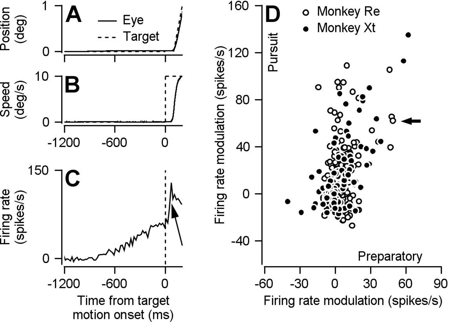
Preparatory- and pursuit-related responses in our FEFSEM population.
(A, B) Continuous and dashed traces plot trial-averaged position (A) and speed (B) of the eye and target for one example experiment. (C) Trial-averaged firing rate as a function of time for one example neuron. The arrow points out the pursuit-related component of firing. (D) Solid and open symbols plot pursuit-related firing rate modulation as a function of preparatory-related firing rate modulation for the population of neurons recorded in monkeys Xt (Spearman’s correlation coefficient = 0.55, p = 4.5 x 10⁻¹⁰ , n = 110 data points from 66 neurons) and Re (Spearman’s correlation coefficient = 0.17, p = .02, n = 187 data points from 80 neurons). The black arrow indicates the example neuron from panel C. Pursuit firing rate modulation was calculated as the average firing rate 51-150 ms after motion onset minus the average firing rate during the last 100 ms of fixation. Preparatory firing rate modulation was calculated as the average firing rate during the last 100 ms of fixation minus the average firing rate during 151-250 ms after fixation onset. Panel D is adapted from Darlington et al. (2018), except that here the analysis is performed during different behavioral conditions from the same data set and slightly different epochs are used to calculate pursuit firing rate modulation.
-
Figure 1—source data 1
Source data for Figure 1.
- https://cdn.elifesciences.org/articles/50962/elife-50962-fig1-data1-v2.mat
Figure 2 with 1 supplement
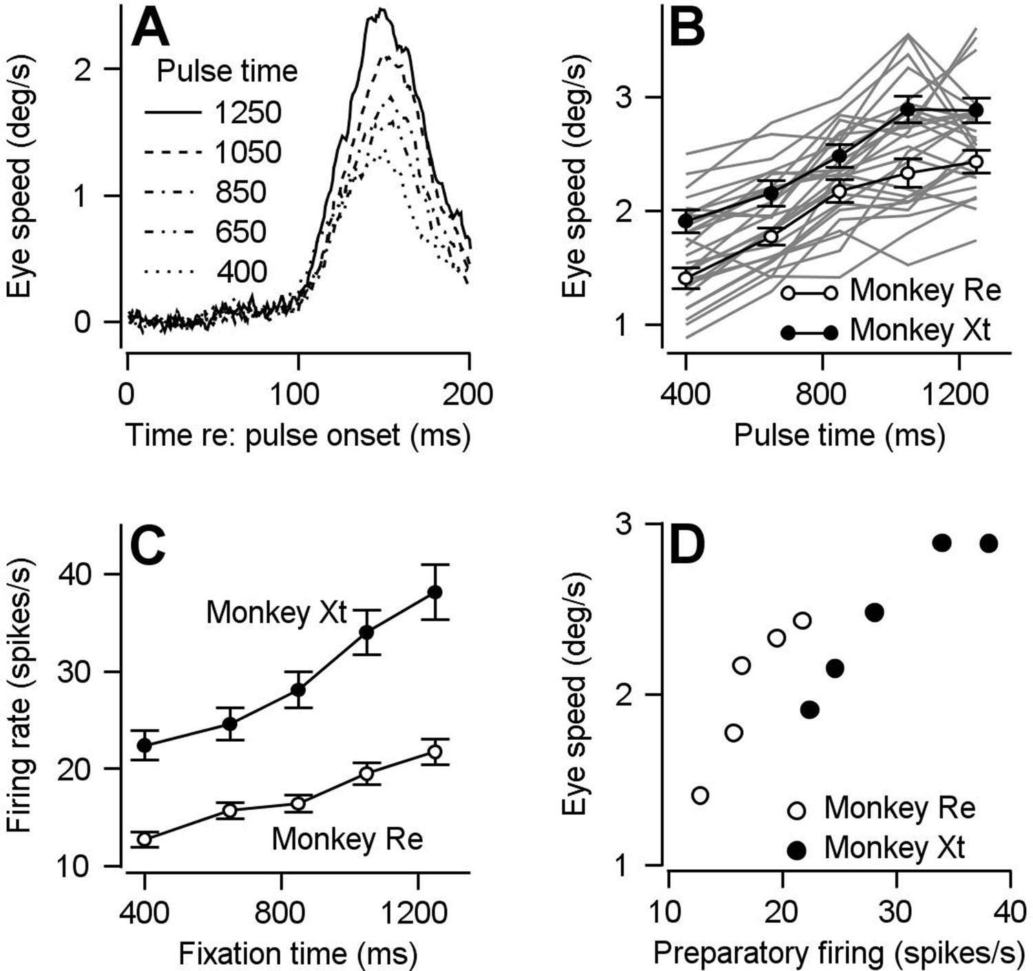
Comparison of time course of visual-motor gain and preparatory activity during fixation at various times after fixation onset.
We probed visual-motor gain by measuring eye speed responses to brief target motions delivered at different times. (A) Different line styles plot trial-averaged eye speed traces aligned to the onset of a pulse of visual motion pulse delivered at different fixation times for one example behavioral experiment. (B) Filled (monkey Xt) and open (monkey Re) symbols plot eye speed averaged across experiments in response to visual motion pulses as a function of the fixation time when the pulse occurred. Error bars represent S.E.M (n = 15 behavioral experiments in Monkey Re and 12 behavioral experiments in Monkey Xt). Eye speeds were measured as the peak response in the interval from motion pulse onset to 200 ms after pulse onset. Light gray curves plot the data from individual experiments. (C) Filled (monkey Xt) and open (monkey Re) symbols plot average preparatory firing rate as a function of fixation time. Data were averaged across all neurons that increased their firing rate across fixation (n = 135 data points in 66 neurons for monkey Re and n = 67 data points in 45 neurons for monkey Xt). Firing rates were calculated as the average firing rate during the last 100 ms of fixation. (D) Filled and open symbols replot the eye speed data from panel B as a function of the firing rates from panel C for each fixation time for the two monkeys.
-
Figure 2—source data 1
Source data for Figure 2.
- https://cdn.elifesciences.org/articles/50962/elife-50962-fig2-data1-v2.mat
Figure 2—figure supplement 1
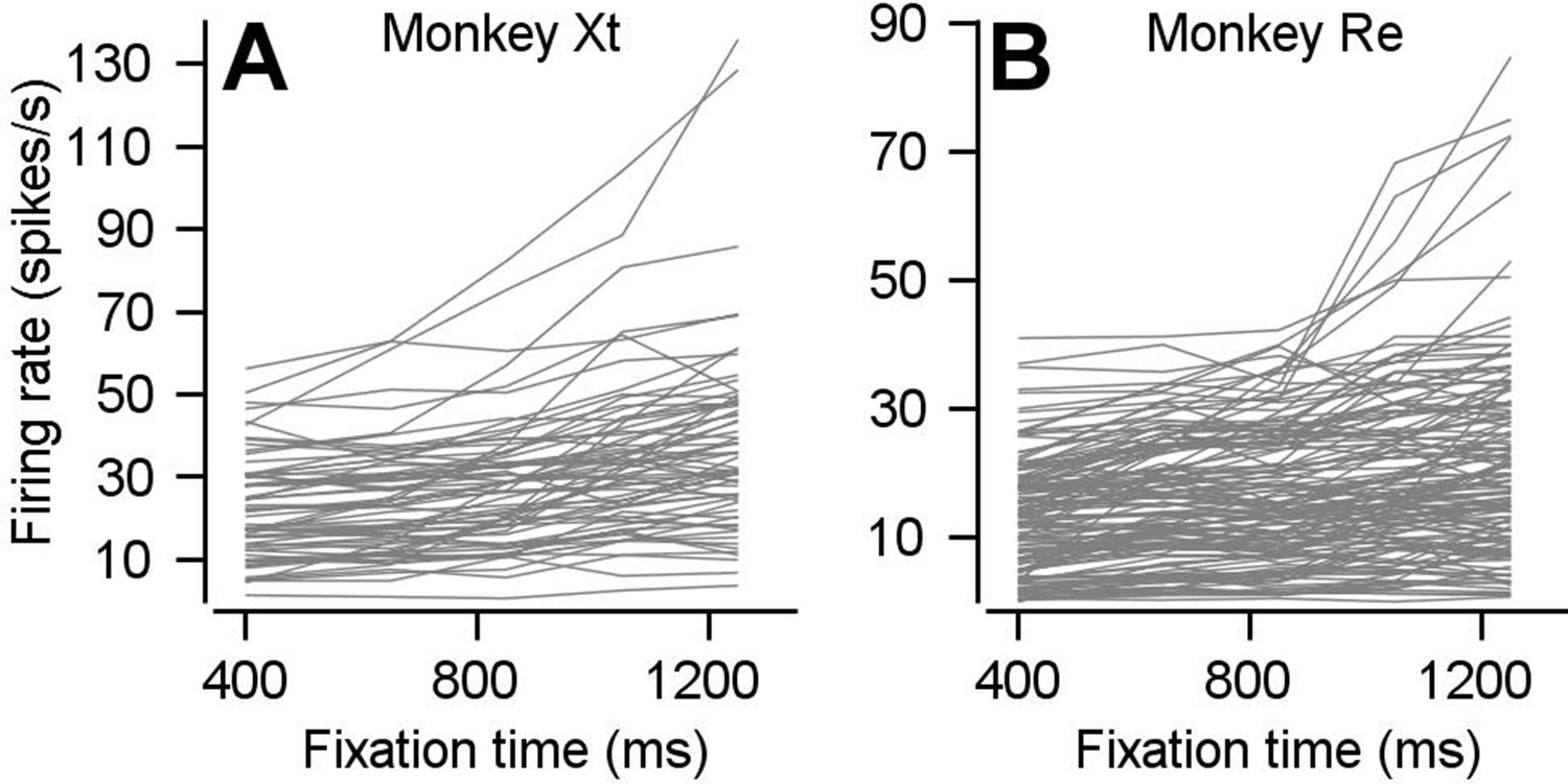
Preparatory firing rate for each neuron with positive preparatory modulation.
(A, B) Curves plot average preparatory firing rate as a function of fixation time for each neuron that went into Figure 2C for monkeys Xt (A) and Re (B).
Figure 3

Parallel effects of expected target speed on visual-motor gain and preparatory neural activity.
(A) Top and bottom panels plot the blend of target speeds during the fast- and slow-contexts used to control the expectation of target speed. (B) Green and blue traces show results for the fast- versus slow-context and plot the preparatory firing rate as a function of time during fixation, averaged separately across neurons that exhibit firing rate increases and decreases across fixation. Error-bands represent S.E.M (increase cells: n = 191 samples from 111 cells, decrease cells: n = 106 samples from 63 cells). Preparatory modulation was calculated for each sample as the average firing rate during the last 100 ms of fixation minus the average firing rate during 151–250 ms after fixation onset. Samples with positive and negative modulation were classified as increase and decrease cells. According to this classification, firing rate increased during fixation for 82 cells, decreased during fixation for 34 cells, and increased during fixation for some directions and decreased for other directions in 29 cells. (C) Green and blue traces show data obtained during the fast and slow contexts and plot the experiment-averaged eye speed responses aligned to the onset of the visual motion pulse. Error-bands represent S.E.M. (D) Open (monkey Re) and solid (monkey Xt) data symbols plot the trial-averaged peak eye speed response to visual motion pulses during the slow-context as a function of that during the fast context. Each symbol shows data for a single experiment (n = 15 behavioral experiments in Monkey Re and n = 11 behavioral experiments in Monkey Xt). Dashed line indicates unity.
-
Figure 3—source data 1
Source data for Figure 3.
- https://cdn.elifesciences.org/articles/50962/elife-50962-fig3-data1-v2.mat
Figure 4

Parallels in directional specificity of eye speed responses to visual motion pulses and FEFSEM preparatory activity.
(A) Filled circles, open circles, and open triangles plot eye speed in response to visual motion pulses delivered during fixation in the same, orthogonal, and opposite direction as the expected pursuit direction. Data are averaged across experiments for both monkeys and error-bars plot S.E.M (n = 30 behavioral experiments across two monkeys). Fixation times were binned across 200 ms and plotted on the x-axis at the value in the middle of the bin. (B) Symbols plot average preparatory modulation of firing rate versus the direction of the experiment relative to the preferred direction of the cell. Error-bars represent the S.E.M. (Same: n = 119 samples across 97 neurons, Orthogonal: n = 111 samples across 79 neurons, Opposite n = 67 samples across 62 neurons). (C) Bar graph plots the percentage of variance explained by each of the 10 components obtained by demixed principal component analaysis (dPCA). Filled and open bars designate direction-dependent versus direction-independent variance contributions to each component. (D), (E), (F) Black and red curves plot the projection of FEFSEM preparatory activity during single-direction blocks of trials that were toward or away from the preferred direction of each cell onto the first (D), second (E), and third (F) components obtained used dPCA.
-
Figure 4—source data 1
Source data for Figure 4.
- https://cdn.elifesciences.org/articles/50962/elife-50962-fig4-data1-v2.mat
Figure 5
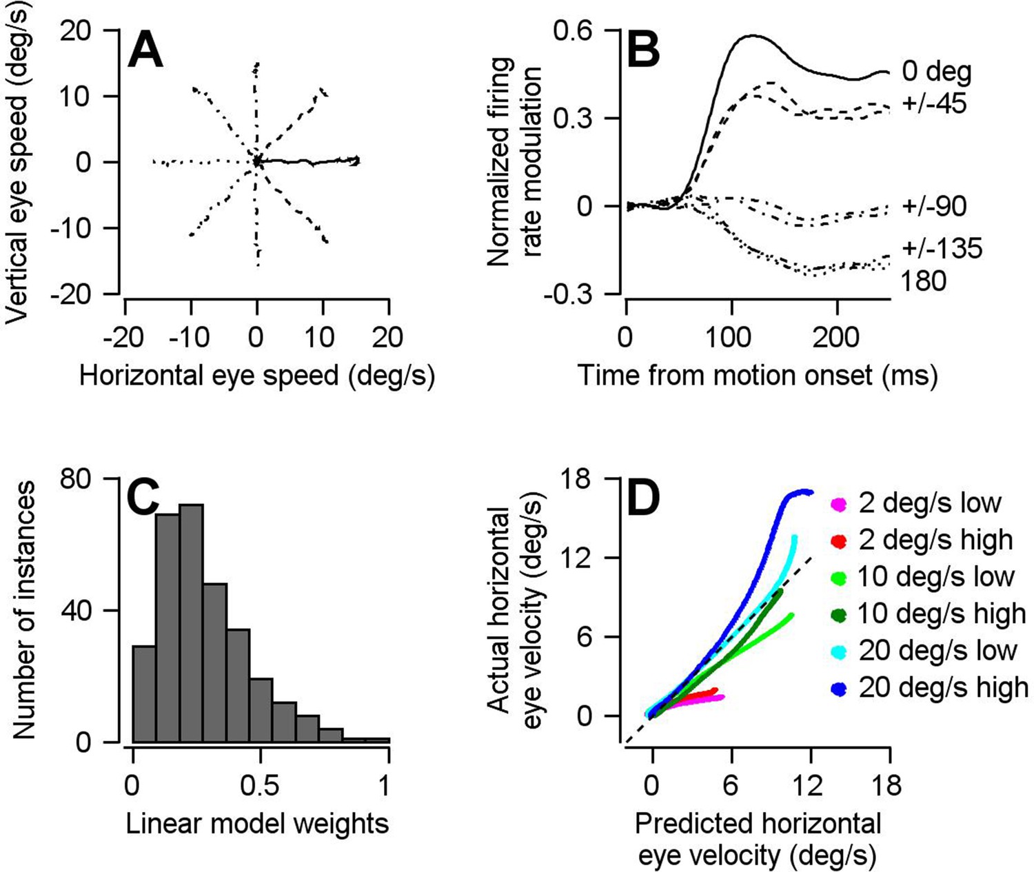
The optimal linear model for converting the population activity in FEFSEM into eye velocity.
(A) Different line styles plot trial-averaged horizontal versus vertical eye velocity for smooth pursuit eye movement to 15 deg/s target motion in eight different directions (4 cardinal and four oblique directions). (B) Traces with the same line styles as in A plot the population trial-averaged firing rate after rotating directions to align the preferred direction of each cell at 0 deg (n = 146 FEFSEM neurons collected in two monkeys). (C) Histogram plots the distribution of calculated linear model weight magnitudes across our population of FEFSEM units. (D) Cross validation of the optimal linear model. The curves plot the horizontal eye velocity predicted during the single-direction block of trials by the model versus actual trial-averaged horizontal eye velocity. Different colored traces differentiate among 6 combinations of target contrast and speed.
-
Figure 5—source data 1
Source data for Figure 5.
- https://cdn.elifesciences.org/articles/50962/elife-50962-fig5-data1-v2.mat
Figure 6 with 3 supplements
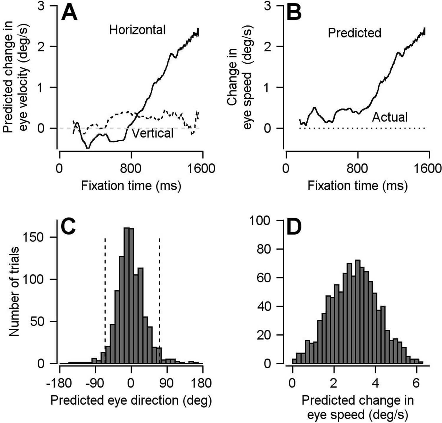
Result of using optimal linear model to transform preparatory activity in FEFSEM into a prediction of eye velocity during preparation for movement.
(A) Solid and dashed traces plot the linear model’s predictions for horizontal and vertical eye velocity during fixation. (B) Solid and dotted traces plot the linear model’s prediction for eye speed during fixation and the actual eye speed during fixation. (C, D) Histograms plot the distributions of predicted eye movement direction and speed during fixation from 1000 bootstrapped iterations of preparatory modulation of activity for single trials. The dashed lines in c demarcate the middle 95% of the distribution.
-
Figure 6—source data 1
Source data for Figure 6.
- https://cdn.elifesciences.org/articles/50962/elife-50962-fig6-data1-v2.mat
Figure 6—figure supplement 1
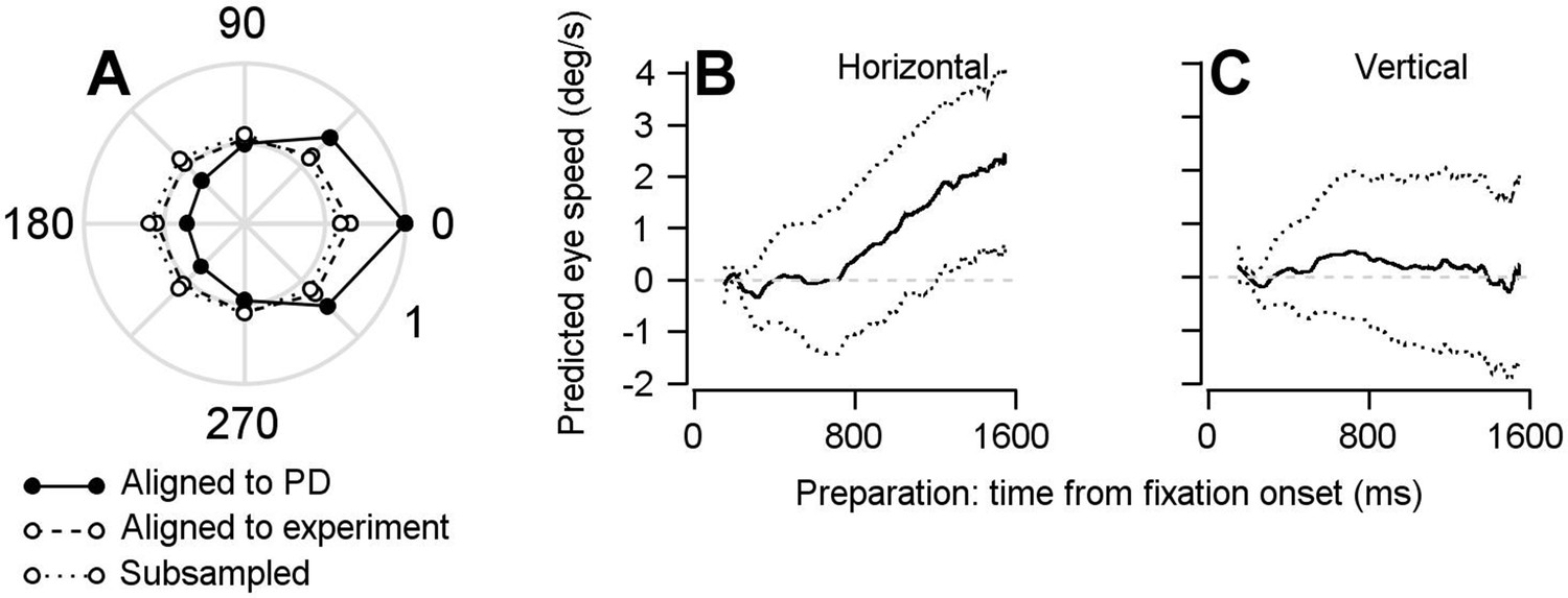
Findings based on the optimal linear model are not the result of oversampling data from neurons’ preferred directions.
We ran the single-direction experiments at various points along the tuning curve of the cells that were being recorded. If we had only run the single-direction experiment in the preferred direction of our recorded cells then we might have missed a part of the true population response that could be responsible for rotating the dimension of the population preparatory activity into a dimension that, indeed, would be orthogonal to the pursuit-related activity. (A) Polar plot showing normalized firing rates averaged over the period of 50–150 ms after visual motion onset during the direction tuning block. Symbols connected by solid and dashed lines represent data aligned to estimated preferred direction or the direction of the repeated-direction block. Data were averaged across 297 data points from 146 cells. Our success in capturing the full population response is evident in the fact that the direction tuning of the population aligned to the single-direction experiment is considerably flatter than the population tuning curve we obtain if we aligned the responses of all neurons to their preferred directions. To further ensure that our findings are not due to an oversampling of the preferred direction of the cells in our population during the repeated-direction experiment, we performed a control analysis by subsampling our FEFSEM population to ensure an equal representation of preferred directions and produce an even flatter population direction tuning curve. We split our population into eight groups based on the difference between preferred directions and the direction of the single-direction experiment. We then randomly sampled 20 units from each of the eight groups, resulting in populations of 160 units. Points connected by dotted lines show normalized firing rates during the direction tuning block aligned to the direction of the repeated-direction block averaged across our subsampled, bootstrapped population. (B, C) Repeating the linear model analysis shown in Figures 5–6 on the uniformly-subsampled population yielded the same conclusion: FEFSEM preparatory-activity predicts movement during fixation; the predicted movement is in the direction of the upcoming target and eye motion. Solid traces plot the mean of the bootstrapped linear model’s predictions for horizontal (B) and vertical (C) eye speed during fixation for the subsampled population. Dotted traces show the middle 95% distributions generated by the bootstrap (n = 1000 iterations).
-
Figure 6—figure supplement 1—source data 1
Source data for Figure 6—figure supplement 1.
- https://cdn.elifesciences.org/articles/50962/elife-50962-fig6-figsupp1-data1-v2.mat
Figure 6—figure supplement 2
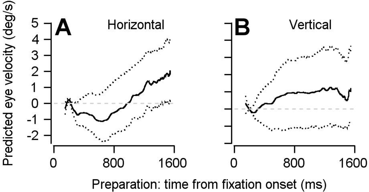
Findings based on the optimal linear model are not the result of including multiple data points from each neuron in our pseudo-population.
The pseudo-population we constructed for the analyses performed in Figures 5 and 6 included multiple data points collected from the same neurons as if they were independent units, under assumptions described in the text. Here, we shown that this analytical choice had no impact on our findings. We have repeated our optimal linear model using a bootstrap approach, in which each neuron could contribute at most one data point. 140 of the 146 neurons were randomly sampled without replacement for each bootstrap. Data from a single experiment was then randomly chosen from each of the 140 neurons. In other words, each of the 140 units in the pseudo-population for each bootstrap is truly an independent neuron. The optimal linear model analysis was then performed as in Figures 5 and 6. (A, B) Repeating the linear model analysis with this modified bootstrap approach yielded the same conclusion: FEFSEM preparatory activity predicts movement during fixation that is in the same direction as the upcoming target and eye motion. Solid traces plot the mean of the bootstrapped linear model’s predictions for horizontal (A) and vertical (B) eye velocity during fixation. Dotted traces show the middle 95% distributions generated by the bootstrap (n = 1000 iterations).
-
Figure 6—figure supplement 2—source data 1
Source data for Figure 6—figure supplement 2.
- https://cdn.elifesciences.org/articles/50962/elife-50962-fig6-figsupp2-data1-v2.mat
Figure 6—figure supplement 3

Repeating the optimal linear analysis in a manner more congruent to that used in Kaufman et al. (2014) produces the same conclusions.
For reasons outlined in the text, we made several modifications in applying the optimal linear model analysis from Kaufman et al. (2014) to ask the question: does preparatory activity evolve in a way that predicts movement? Here we present a supplementary analysis that is more congruent with the analysis performed in the Kaufman et al. paper. First, we used only the data from the single-direction blocks of trials, instead of fitting to the 8-direction blocks and predicting the data from the single-direction blocks as we had done before. Second, we performed PCA on the neural data before fitting to movement parameters. In this way the W from equation (3) is now solved from the equation , where is the lower-dimensional representation of the neural population response during the movement epoch obtained from PCA. E is the eye velocity (A and B) or eye speed (C and D) from the single-direction pursuit task. We are fortunate that the kinematics of the movement uniquely reflect the action of the extraocular eye muscles and are already low-dimensional (2-dimensional for velocity, 1-dimensional for speed). Therefore, we did not need to perform PCA on the movement data (E). In accordance with Kaufman et al. (2014) we chose the dimensions of based on the movement dimensions in order to have an equal number of dimensions in the row and null space of the weight matrix. For fitting to eye velocity and speed, we chose the dimensionality of to be 4 and 2, respectively. We then projected the low-dimensional representation of the neural population response during the preparatory epoch of the single-direction pursuit task onto the row and null spaces of W. Because the curves in panels A and C deviated from zero systematically, our supplementary analysis reaches the same conclusion as Figures 5 and 6: preparatory activity evolves in a way that predicts movement when there is none. In the words of Kaufman et al. (2014), FEFSEM preparatory activity is not confined to the null space. (A), (B) Solid and dashed traces plot the projection of the low-dimensional representation of population preparatory activity onto the row (A) and null (B) spaces of the weight matrix obtained from fitting to horizontal (solid) and vertical (dashed) eye velocity. (C), (D) Solid and dashed traces plot the projection of the low-dimensional representation of population preparatory activity onto the row (C) and null (D) spaces of the weight matrix obtained from fitting to eye speed. In both analyses, the magnitude of projection of preparatory activity onto the null space increase very early in fixation and decays back to zero as preparation progresses. In contrast, the projection onto the row space steadily increases as preparation progresses. Importantly, the prediction for eye velocity and speed obtained by projection onto the row space is in the direction of the ensuing target motion (0 degrees, right) and positive, respectively.
-
Figure 6—figure supplement 3—source data 1
Source data for Figure 6—figure supplement 3.
- https://cdn.elifesciences.org/articles/50962/elife-50962-fig6-figsupp3-data1-v2.mat
Figure 7 with 1 supplement
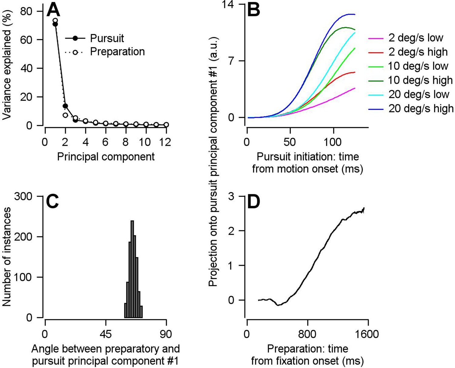
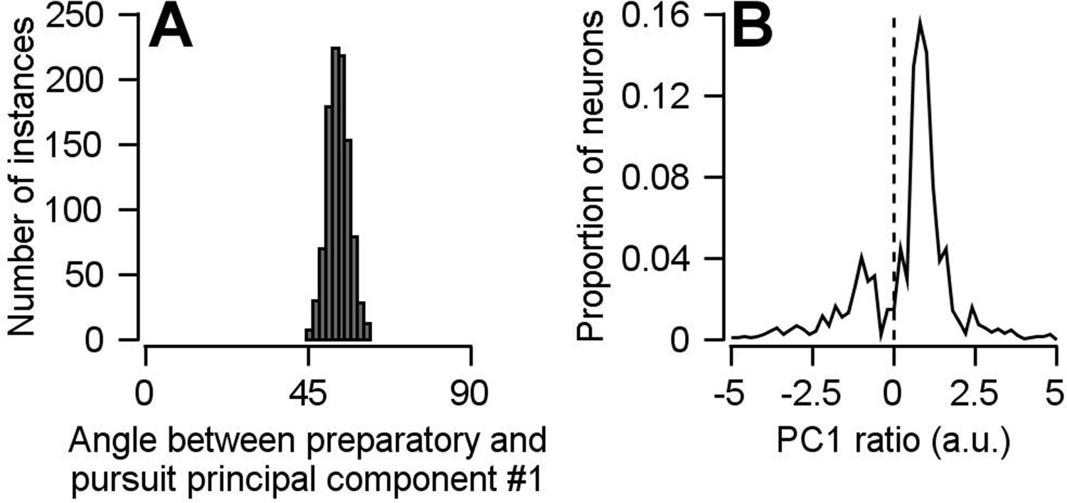
Direct assessment of preparatory- versus pursuit-related neural dimensions through comparison of principal components for preparatory- and pursuit-related population activity in FEFSEM.
(A) Solid and open symbols plot the percentage of the total pursuit-related and preparatory response variances explained by each principal component. Beyond principal component 3, the open symbols obscure the filled symbols. (B) Different colored traces plot projection of pursuit-related population firing rates in response to low-contrast and high-contrast target motion of 20, 10, and 2 deg/s onto the first pursuit principal component. (C) Histogram plots the distribution of the angle between the first pursuit-related and preparatory principal components across 1000 bootstrapped iterations. (D) Projection of population preparatory firing rates during fixation onto the first principal component of pursuit-related responses.
-
Figure 7—source data 1
Source data for Figure 7.
- https://cdn.elifesciences.org/articles/50962/elife-50962-fig7-data1-v2.mat
Figure 7—figure supplement 1
Findings based on the principal component analysis are not the result of including multiple data points from each neuron in our pseudo-population.
The pseudo-population we constructed for the analyses performed in Figures 7 and 8 included multiple data points collected from the same neurons as if they were independent units, under assumptions described in the text. Here, we show that this analytical choice had no impact on our findings. We have repeated our principal component analyses using a bootstrap approach, in which each neuron could contribute at most one data point. 140 of the 146 neurons were randomly sampled without replacement for each bootstrap. Data from a single experiment was then randomly chosen from each of the 140 neurons. In other words, each of the 140 units in the pseudo-population for each bootstrap is truly an independent neuron. The principal component analyses was then performed as in Figures 7 and 8. (A) Repeating the principal component analysis with this modified bootstrap approach yielded the same conclusion: there is a partial reorganization of neural population dimensions between preparation and movement. The histogram shows the distribution of angles between the first preparatory- and pursuit-related principal components. (B) Performing the principal component analysis using this modified bootstrap approach also unveiled the existence of a small subpopulation that’s predominantly responsible for the partial reorganization of neural dimensions between preparation and movement. The solid line plots the distribution of PCPrep1/PCPurs1 ratios averaged across the 1000 bootstraps.
-
Figure 7—figure supplement 1—source data 1
Source data for Figure 7—figure supplement 1.
- https://cdn.elifesciences.org/articles/50962/elife-50962-fig7-figsupp1-data1-v2.mat
Figure 8
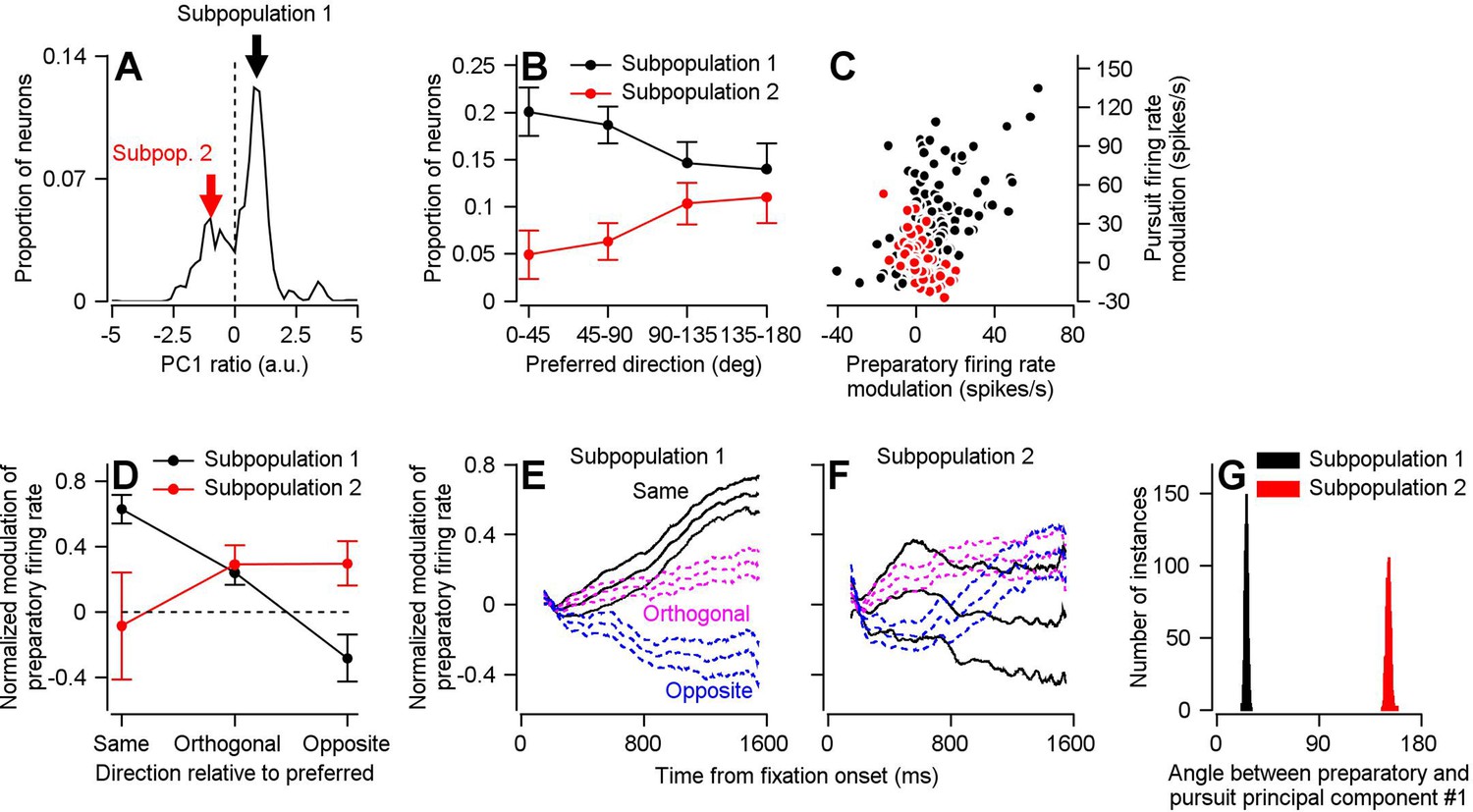
Two subpopulations of FEFSEM neurons with different relationships between preparatory and pursuit-related activity.
(A) The distribution of PCPrep1/PCPurs1 ratios averaged across 1000 bootstrapped iterations. The dashed line indicates a ratio of 0, the point where we split our FEFSEM population into two subpopulations. (B) Black and red symbols summarize the distributions of preferred directions relative to the direction of the single-direction experiment for units in Subpopulations 1 and 2 in the bootstrap analysis. Error bars represent the middle 95% distribution obtained from our bootstrap analysis (n = 1000 iterations). (C) Black and red symbols plot preparatory- versus pursuit-related firing rate modulations for Subpopulations 1 and 2 in our full FEFSEM data set (n = 207 data points from 130 neurons for Subpopulation 1 and n = 90 data points from 65 neurons for Subpopulation 2). Panel C plots the same data from Figure 1D, except here it has been separated into Subpopulations 1 and 2 (D) Black and red symbols plot data for subpopulations 1 and 2 and show the normalized preparatory modulation of firing rate versus the direction of the experiment relative to the preferred direction of the cell. Error-bars represent the middle 95% of the bootstrapped distribution (n = 1000 iterations). (E), (F) Black, magenta, and blue traces plot normalized modulation of preparatory firing rate as a function of time from fixation onset when experiments were run in the same, orthogonal, and opposite direction as the preferred direction of the neuron. Data were averaged separately across neurons in Subpopulations 1 (E) and 2 (F). For each direction, the middle trace is the average and the flanking traces border the middle 95% of the bootstrapped distribution, n = 1000 iterations). (G) Black and red histograms plot the distribution of the angle between the first pursuit-related and preparatory principal components for Subpopulations 1 and 2 across 1000 bootstrapped iterations.
-
Figure 8—source data 1
Source data for Figure 8.
- https://cdn.elifesciences.org/articles/50962/elife-50962-fig8-data1-v2.mat
Figure 9
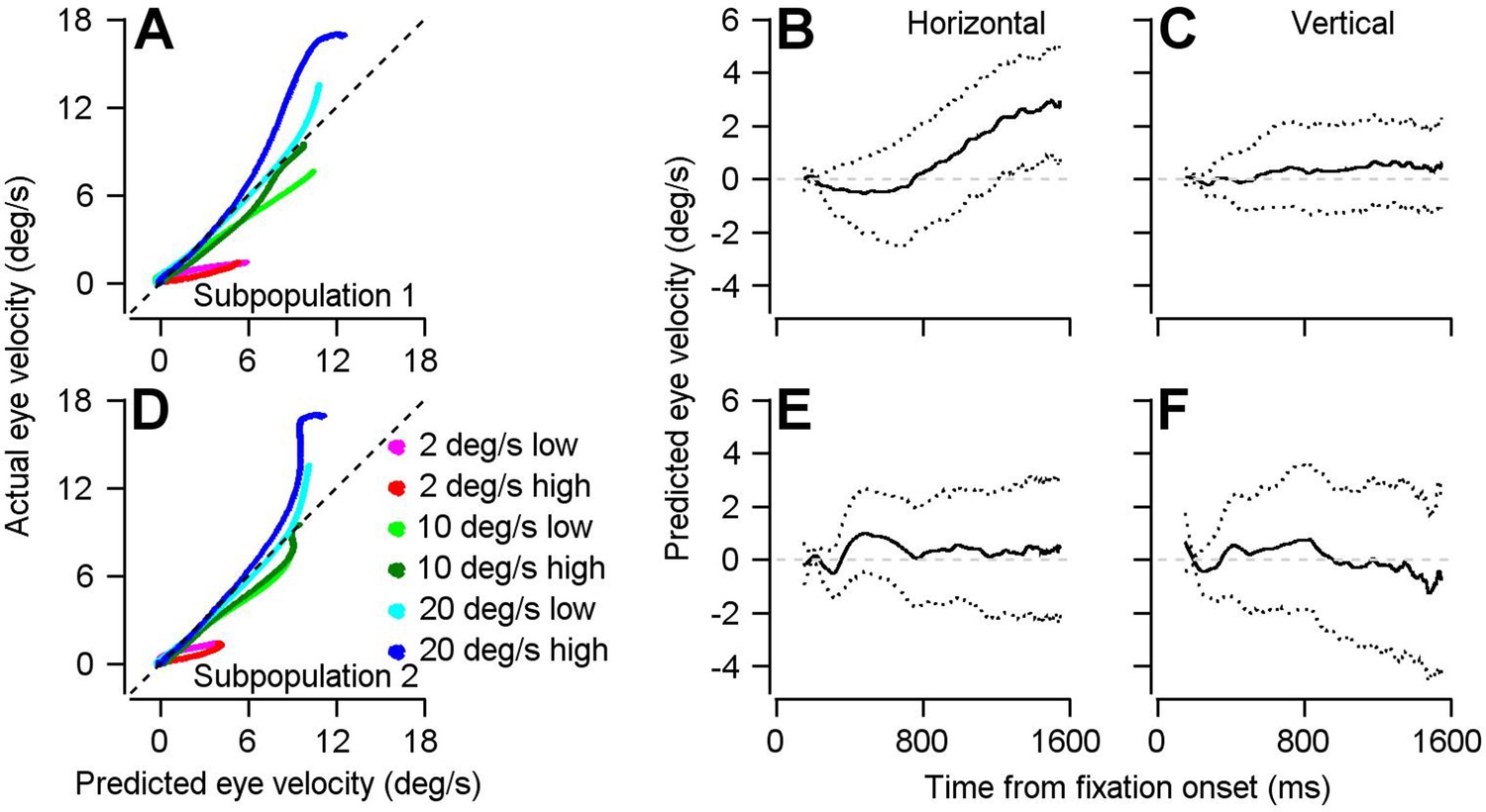
Result of using optimal linear model to transform preparatory activity in the two subpopulations into a prediction of eye velocity during preparation for movement.
(A, D) The curves plot the horizontal eye velocity predicted during the single-direction block of trials by the model for Subpopulation 1 (A) and Subpopulation 2 (D) versus actual trial-averaged horizontal eye velocity. (B, C, E, F) Solid traces plot the mean of the bootstrapped linear model’s predictions for horizontal (B, E) and vertical (C, F) eye velocity during fixation for Subpopulation 1 (B, C) and Subpopulation 2 (E, F).: Different colored traces in A and D differentiate among 6 combinations of target contrast and speed. Dotted lines in B, C, E, and F plot the middle 95% of the 1000 bootstrapped iterations.
-
Figure 9—source data 1
Source data for Figure 9.
- https://cdn.elifesciences.org/articles/50962/elife-50962-fig9-data1-v2.mat
Author response image 1
Additional files
Download links
A two-part list of links to download the article, or parts of the article, in various formats.
Downloads (link to download the article as PDF)
Open citations (links to open the citations from this article in various online reference manager services)
Cite this article (links to download the citations from this article in formats compatible with various reference manager tools)
Mechanisms that allow cortical preparatory activity without inappropriate movement
eLife 9:e50962.
https://doi.org/10.7554/eLife.50962


