Determinants of MDA impact and designing MDAs towards malaria elimination
- Centre for Tropical Medicine and Global Health, Nuffield Department of Medicine, University of Oxford, United Kingdom
- Mahidol-Oxford Tropical Medicine Research Unit, Faculty of Tropical Medicine, Mahidol University, Thailand
Figures
Figure 1 with 6 supplements
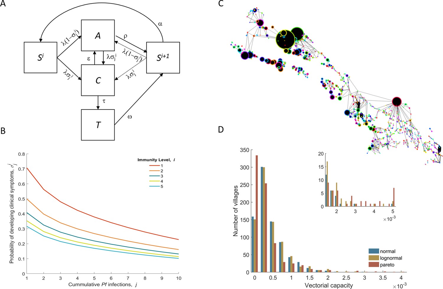
Model structure illustration.
(A) Flow diagram representing the natural history of Plasmodium falciparum infections in human populations. Uninfected individuals (S) can be infected at rate λ, with the probability of developing clinical symptoms (σ) depending on their immunity level i and number of lifetime infections j. Clinical infections (C) can be detected and subsequently treated at rate τ to a treated state (T), or naturally subside into an asymptomatic parasite carrier stage (A) at rate ε. Treated individuals lose their drug at rate ω. After recovery or treatment, individuals become susceptible with an added level of clinical immunity (Si+1). Clinical immunity level decays at rate α. (B) Probability of developing clinical malaria depending on individual’s history of infection (cumulative number of infections) for each immunity level considered here. (C) Village connectivity network. Geo-located villages appear as circles the size of which is proportional to the number of people living there. Edge width reflects individuals’ probability of travel between connected villages. (D) Each village is assigned a specific mosquito density/vectorial capacity, with transmission heterogeneity over space characterized by three different distributions.
Figure 1—figure supplement 1
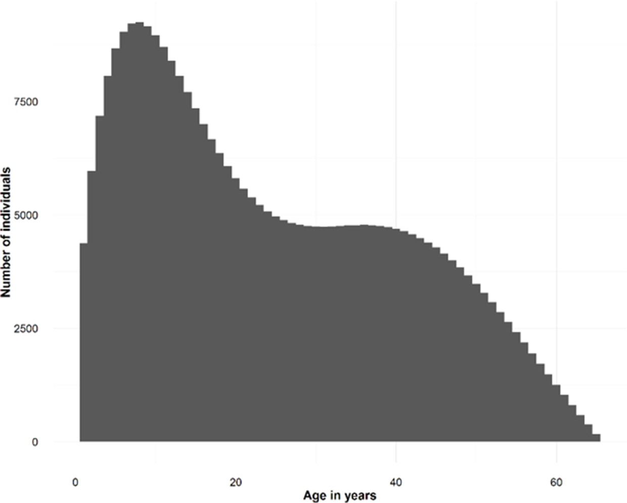
Synthetic population demographics.
Depicts the age distribution of the simulated individuals.
Figure 1—figure supplement 2
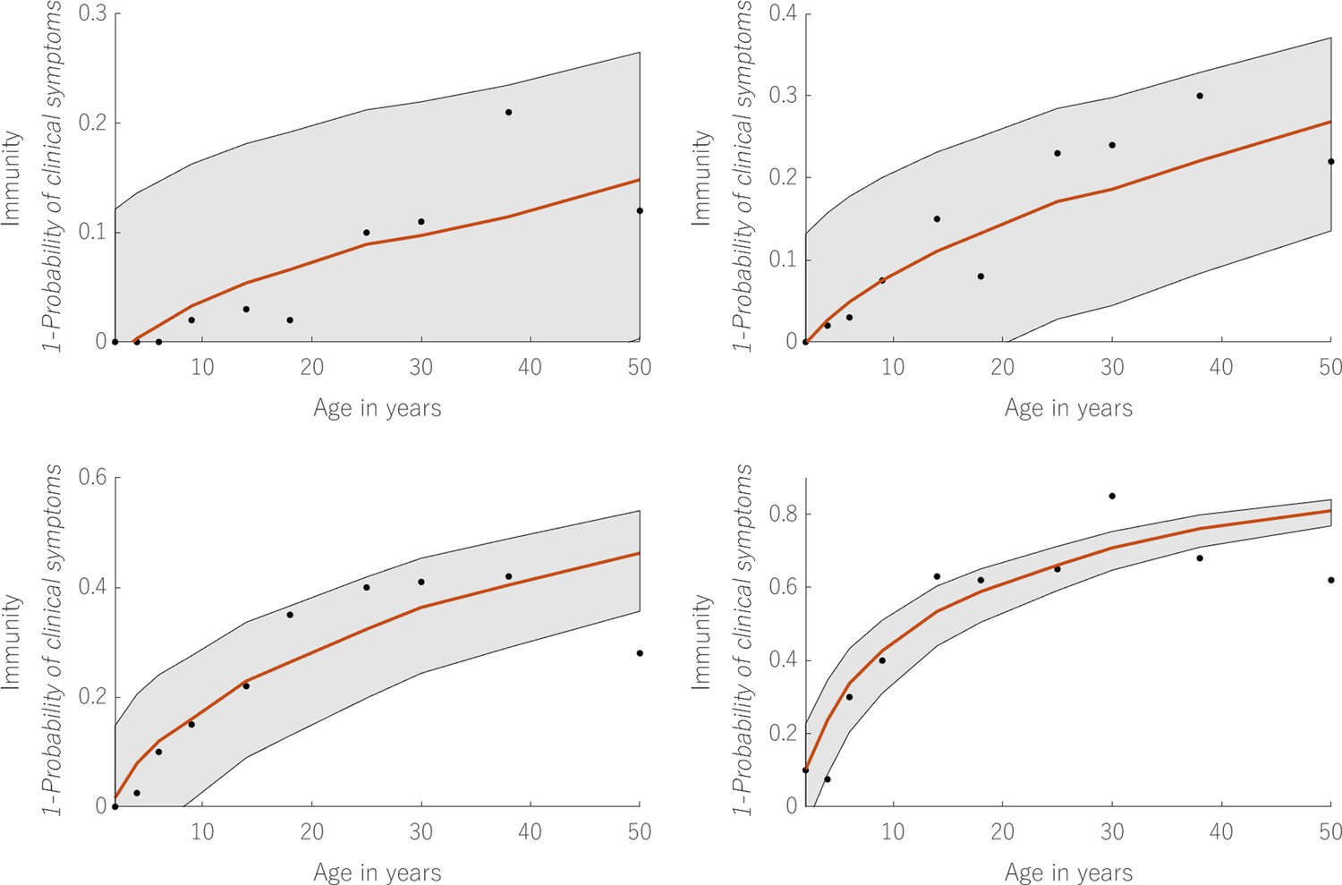
Model fit to immunological data.
Displays the simultaneous fit to 4 measured relationships between age and clinical immunity. The black dots refer to the data points offering a measurement for clinical immunity in each of these endemic settings. The red line shows the output of , for the estimated values of imm_a and imm_b taking as inputs the mean values of cml and lvl (taken from the model output) in individuals of age given by the X-axis. The grey bands represent the 95% credible intervals.
Figure 1—figure supplement 3

Calibrated relationship between EIR and Data.
The black dots depict the data points in the Guerra et al. (2007) database. The colored dots show 100 thousand individual model predictions for the observable prevalence in a village (aggregated over 100 runs with 1000 villages each) with EIR given in the X-axis. These 100 runs scan the biting rate parameter space, increasing the mean biting rate in 1000 village for each run, until a desirable coverage of EIR values is obtained. Each color signifies a different distribution of how mosquito densities vary over space. The more extreme distribution (Pareto) displays a higher variance, more in line with that observed in the data, particularly for low EIR values. This is caused by population movement, with people living in these low EIR villages potentially being infected in very high EIR villages when they visit them.
Figure 1—figure supplement 4
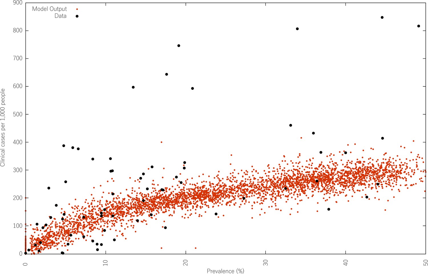
Calibrated relationship between prevalence and clinical malaria incidence.
Compares the predicted clinical malaria case incidence for varying levels of prevalence (red), with the data (black) published in Patil et al. (2009). Much like in the previous figure, 100 thousand individual village model predictions of the observable clinical incidence in a village (aggregated over 100 runs with 1000 villages each) for varying prevalence levels. These 100 runs scan the biting rate parameter space, increasing the mean biting rate in 1000 village for each run, until a desirable coverage of prevalence values is obtained.
Figure 1—figure supplement 5
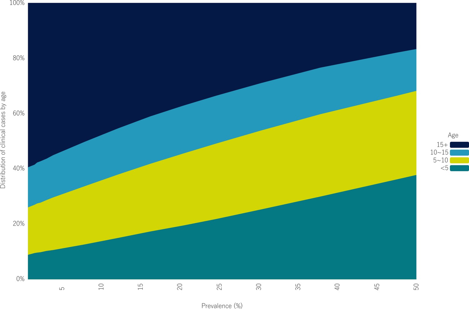
Clinical age profiles for different endemic levels.
Shows how the distribution of malaria clinical cases across age bins changes with increasing all-age true prevalence.
Figure 1—figure supplement 6
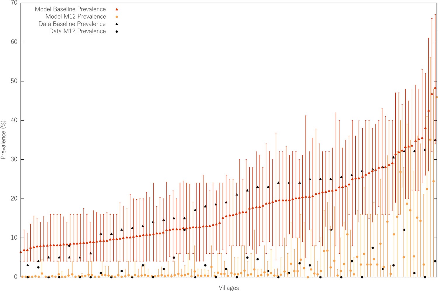
MDA effect size for different values of starting prevalence.
The black triangles and dots refer to the prevalence measured at baseline and at month 12 post MDA in the MDA trials performed in the Thai-Myanmar border (Landier et al., 2018). We refrained from plotting the data error bars here, since the plot is already quite busy. We simulate a targeted MDA strategy in all similar to the one carried out in the aforementioned study, with a prevalence survey carried out in the year prior to MDA start and another exactly 12 months (M12) after the fist MDA round. The prevalence surveys consist of sampling 50 random individuals from each village and assessing the prevalence assuming a diagnostic sensitivity of 85%. For each village, only the runs in which that village was selected for MDA (having a baseline prevalence over 5%) are used to calculate the mean prevalence at baseline and month 12. Note that these are not meant to be the same villages. The modelled villages are synthetic villages with no relation to or input from the original dataset. The only commonality is that the modelled mean prevalence at baseline in the entire population (also including villages that do not receive MDA) is the same as that in the data (~5%).
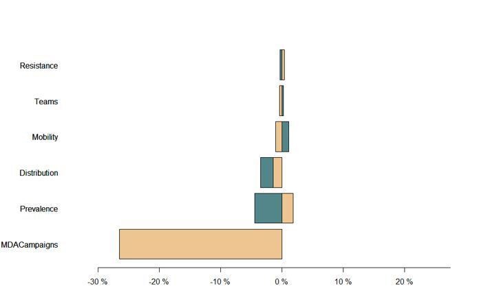
Figure 2 with 5 supplements

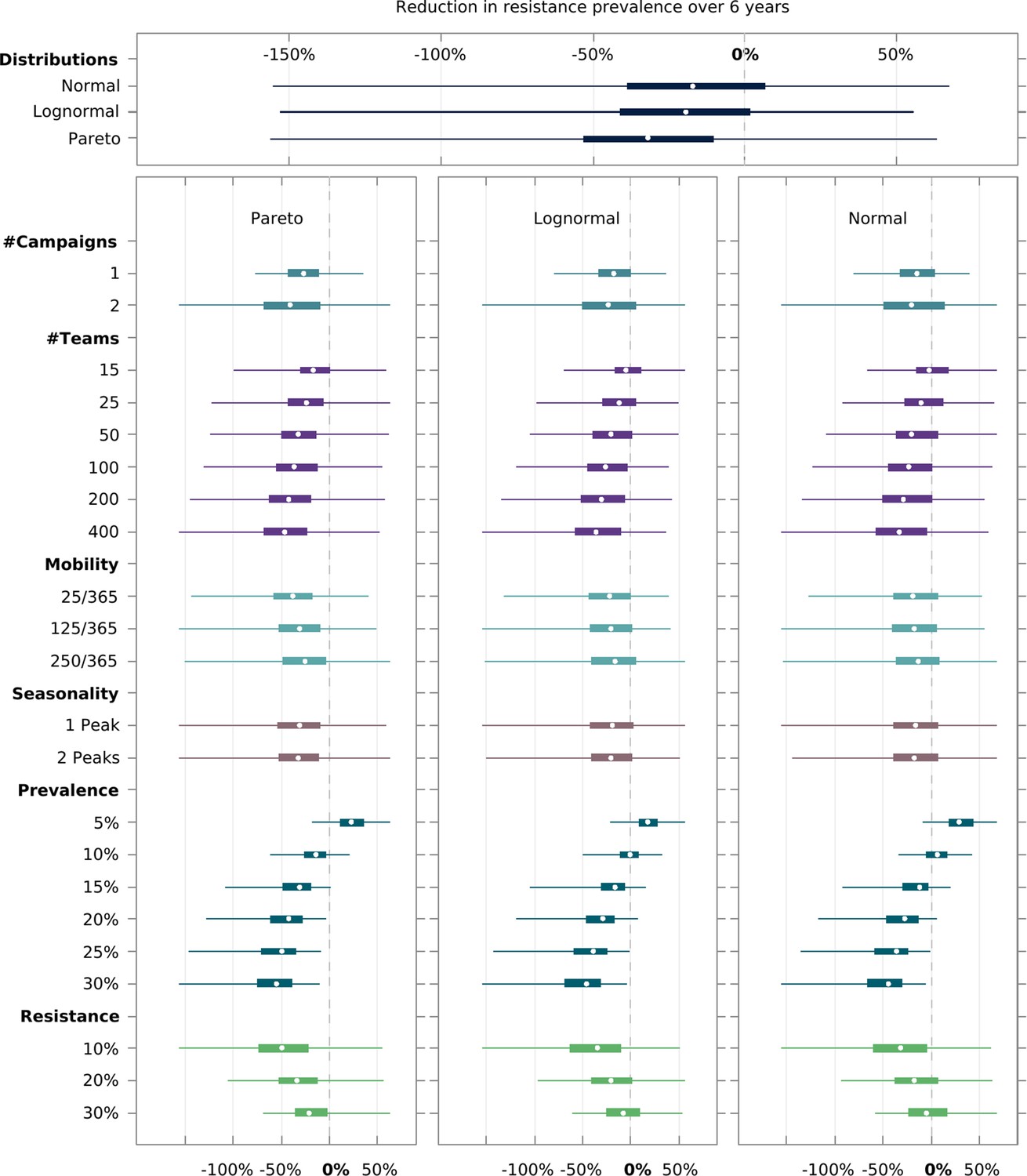
Multivariate sensitivity analysis of the predicted intervention impact on malaria prevalence and artemisinin resistance.
The box plots show the median and interquartile ranges of the proportional reduction in malaria prevalence for all simulated parameter sets. Each parameter set consists of a combination of initial mean prevalence (Prevalence), initial proportion of artemisinin resistance parasites (Resistance), population mobility (Mobility), number of teams deployed in the field (# Teams), number of MDA campaigns (# Campaigns), and number of transmission peaks per year (Seasonality). An overall mean and interquartile range for the effect of transmission heterogeneity, independent of any other parameter, is displayed on the top panel. The reduction in prevalence is evaluated as the proportional difference in the integral in prevalence in the 5 years following MDA relative to the 5 years preceding MDA.
Figure 2—figure supplement 1

Multivariate model sensitivity analysis independent of transmission heterogeneity.
Model outcome (measured as the proportional decrease in parasite prevalence) sensitivity to logistical (Teams – speed of coverage, and number of MDA campaigns), epidemiological (initial mean prevalence in the target area, given in black background over each panel), and behavioral (mobility – daily probability of spending nights in a place other than the habitual residence) parameters. Points and adjacent lines indicate the median and interquantile (5th to 95th) ranges (based on 100 simulations for each parameter set).
Figure 2—figure supplement 2
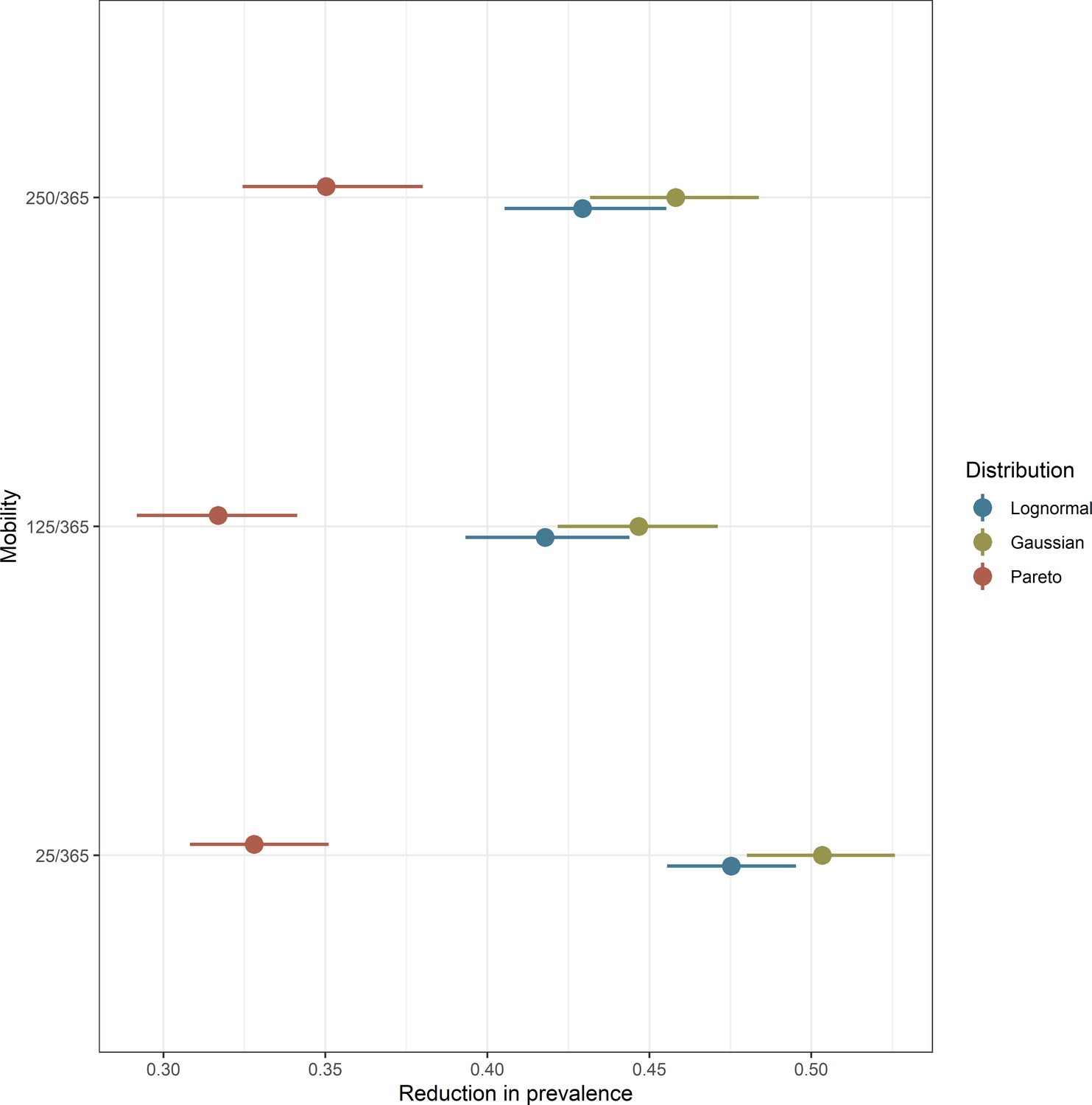
Interplay between population mobility and transmission heterogeneity.
Intervention outcome sensitivity to spatial transmission heterogeneity in settings with different population mobility patterns. The vectorial capacity distributions associated with these simulations are displayed in Figure 1D. Points and adjacent lines indicate the median and interquartile ranges (based on 100 simulations for each parameter set).
Figure 2—figure supplement 3
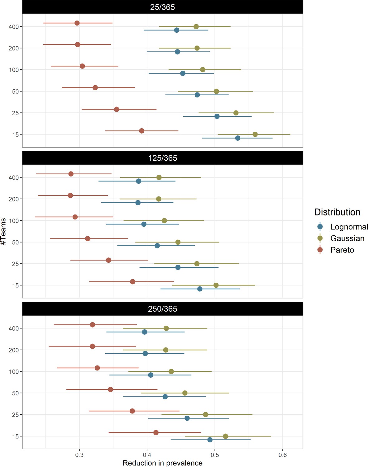
Interplay between logistics and human population topologies.
Model predicted interaction of logistical MDA considerations (speed of coverage – teams) with different population mobility levels (given in black background over each panel) in determining intervention impact for the explored transmission heterogeneity distributions. Points and adjacent lines indicate the median and interquartile ranges (based on 100 simulations for each parameter set).
Figure 2—figure supplement 4
Factors influencing the spread of artemisinin resistance.
In all similar to Figure 2, it shows how the different model parameters modulate the predicted proportional decrease in artemisinin resistance after MDA. Negative numbers then reflect a rise in artemisinin resistant infections from start of the campaign to the end of the simulation (a −100% value indicates a 2-fold increase in the number of resistant parasites).
Figure 2—figure supplement 5
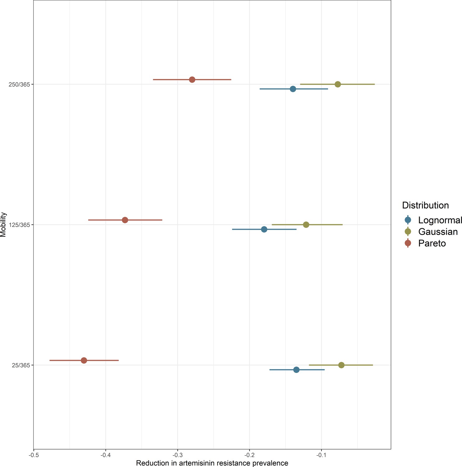
Population movement and mosquito distributions determine artemisinin resistance spread.
Illustrates how human population mobility (y-axis) interacts with how transmission risk is distributed over space (colored groups) to modulate the extent to which artemisinin resistance is able to spread (x-axis).
Figure 3 with 3 supplements
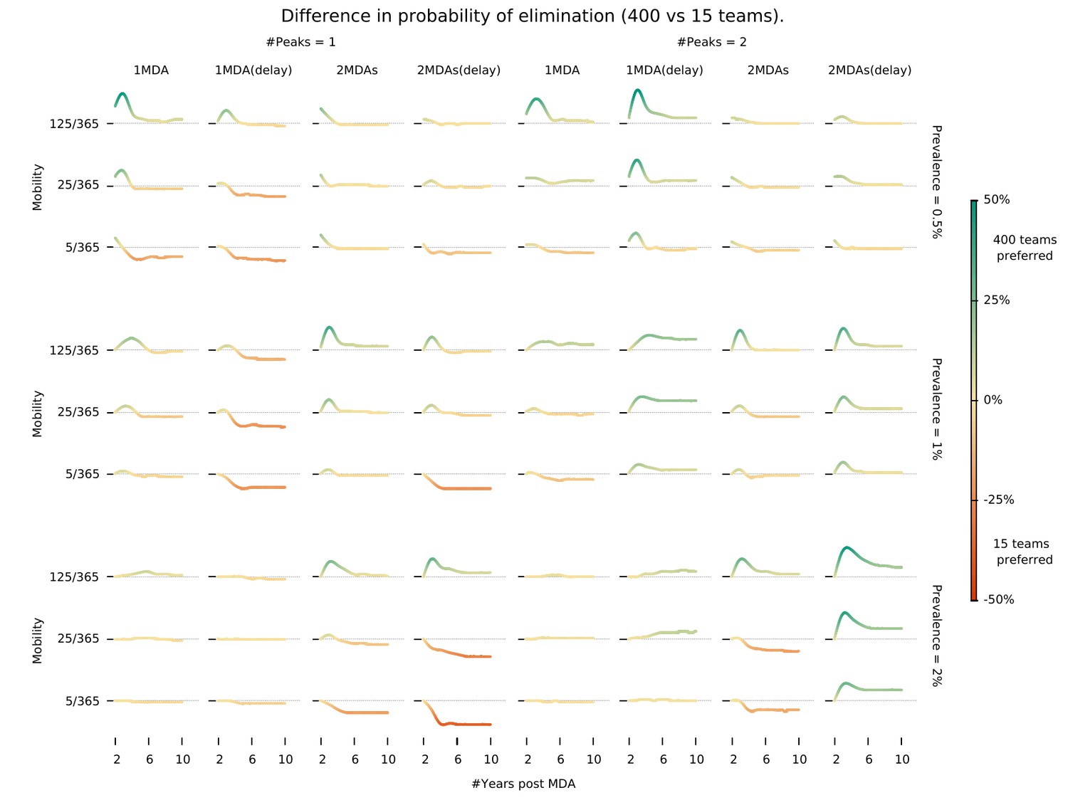
Intervention implementation speed in different epidemiological contexts.
Demonstrates under what conditions using 400 implementation teams is preferable over 15 teams when deploying an MDA campaign. We investigate different epidemiological contexts, characterized by different prevalence and seasonality profiles can be accounted for in deciding the appropriate campaign start day (delay) when maximizing the chances for malaria elimination. ‘MDA (delay)’ means MDA start is delayed to day 60 instead of the default start at the beginning of the calendar year. ‘#Peaks’ indicates the number of transmission peaks per year. The left four columns have 1 peak whereas the right four columns have 2 peaks.
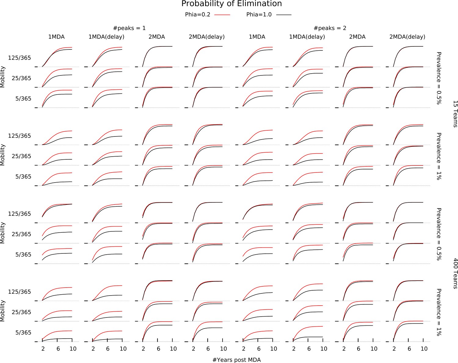
Figure 3—figure supplement 1
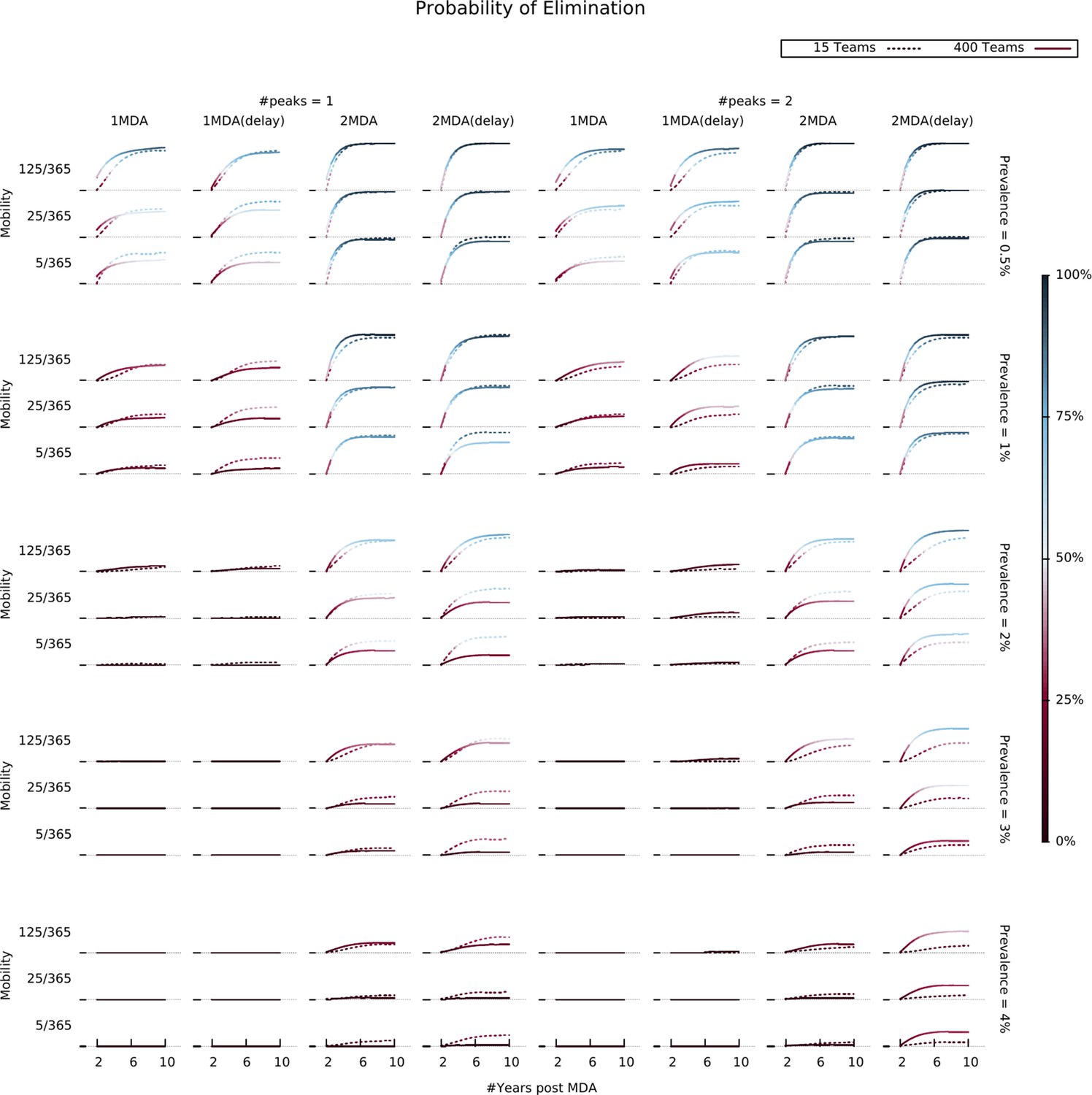
Elimination likelihood over time in different settings.
Illustrates the interaction between human population mobility, seasonality patterns, and MDA operational parameters (number of teams and campaign start time). Colors indicate the proportion of simulations in which elimination was reached for each parameter combination, evaluated at different time points.
Figure 3—figure supplement 2

Relationship between elimination probability and MDA campaign village sequencing.
Shows how the relationship between human population mobility (rows), seasonality patterns (blocks of columns), MDA operational parameters – number of teams (block of rows), campaigns and campaign start time (columns) – and selection for the starting villages for MDA (colors) influences the probability of malaria elimination (y-axis).
Figure 3—figure supplement 3
Relationship between elimination probability and the relative infectivity of asymptomatic infections.
Illustrates how a lower infectiousness assumption for asymptomatic malaria (red line) drives the likelihood of malaria elimination up for independently of the remaining model parameters.
Figure 4 with 3 supplements
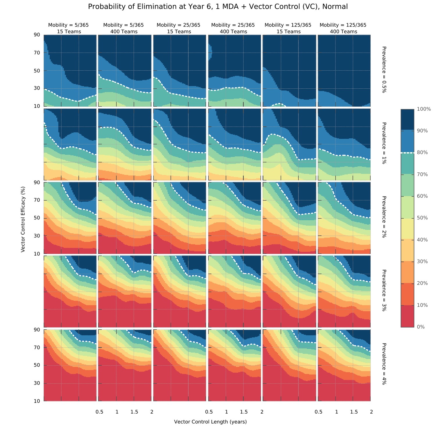
Elimination probability surfaces (Normal distribution of transmission risk over space).
These surface plots show the proportion of simulations (out of 100) in which elimination was achieved within a 5 year time horizon. Hypothetical interventions that decrease the vectorial capacity by a proportion given in the y-axis are maintained for a period of time defined in the x-axis. These transmission blocking interventions are layered on top of a global MDA campaign consisting of 3 ACT rounds in all villages and including widespread village malaria workers. Different panels give different combinations of mean initial malaria prevalence, human population mobility and MDA implementation speed. The white dashed line represents the 80% likelihood of elimination contour line.
Figure 4—figure supplement 1
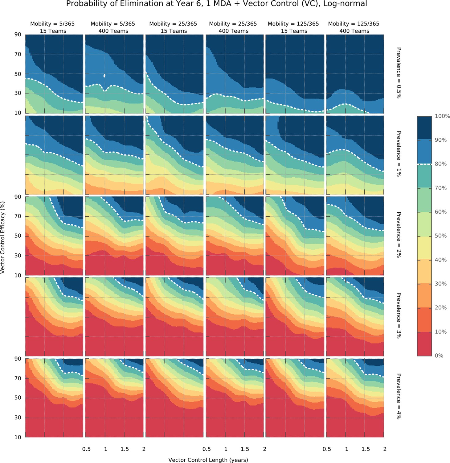
Integrated control elimination surfaces for the Log-normal distribution of transmission risk over space.
Figure 4—figure supplement 2
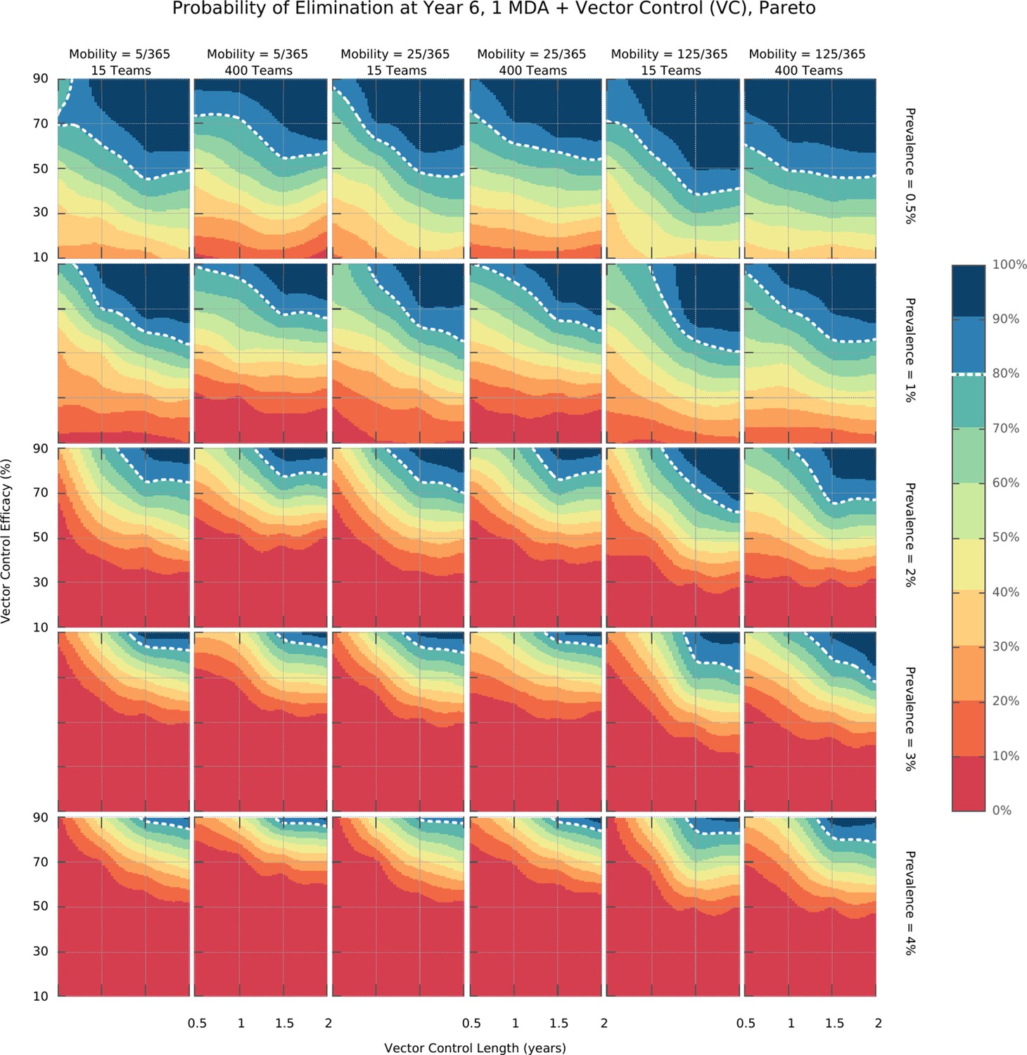
Integrated control elimination surfaces for the Pareto distribution of transmission risk over space.
Figure 4—figure supplement 3
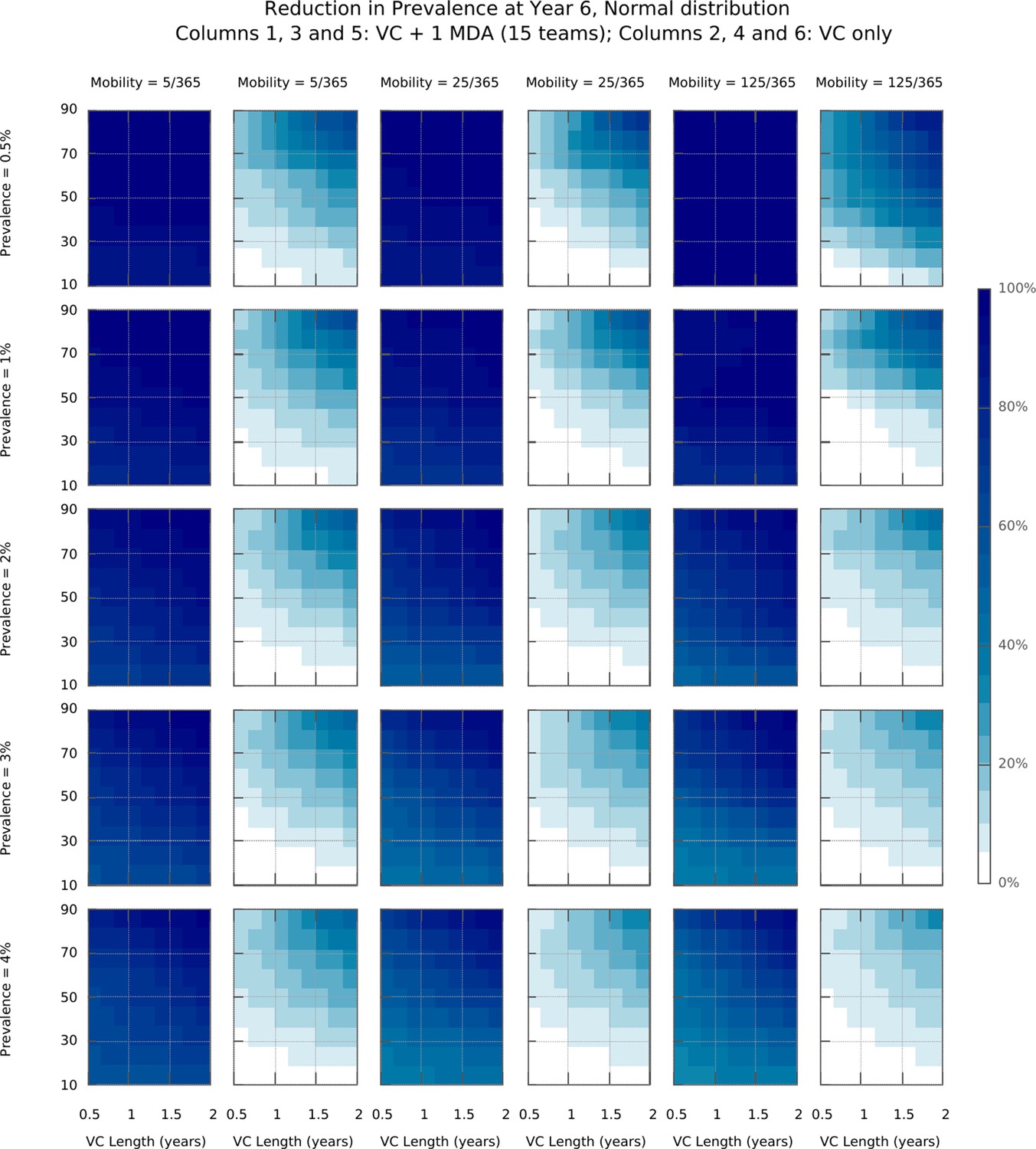
Mean reduction in prevalence in intervention strategies containing either MDA + VC or VC alone.
These surface plots show a drastic improvement in transmission reduction impact when comparing implementations of MDA in setting with varying vector control (VC), against VC only intervention strategies. As shown in columns 2, 4, and 6, implementations of strategies including VC alone are unlikely to achieve elimination.
Figure 5 with 1 supplement
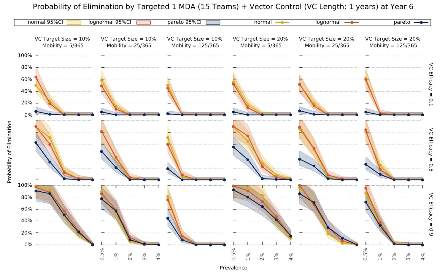
Elimination probability with a targeted approach.
Illustrates the likelihood of elimination within 5 years of an elimination strategy consisting of 3 MDA rounds and a vector control strategy sustained over 1 year. We compare elimination prospects across different prevalence levels, human population mobility, and transmission heterogeneity over space. Vector control (VC) efficacy refers to the coefficient by which vectorial capacity is reduced for the duration of the intervention. The vector control target sizes refer to the quantile of villages, sorted by descending vectorial capacity, targeted by the intervention.
Figure 5—figure supplement 1
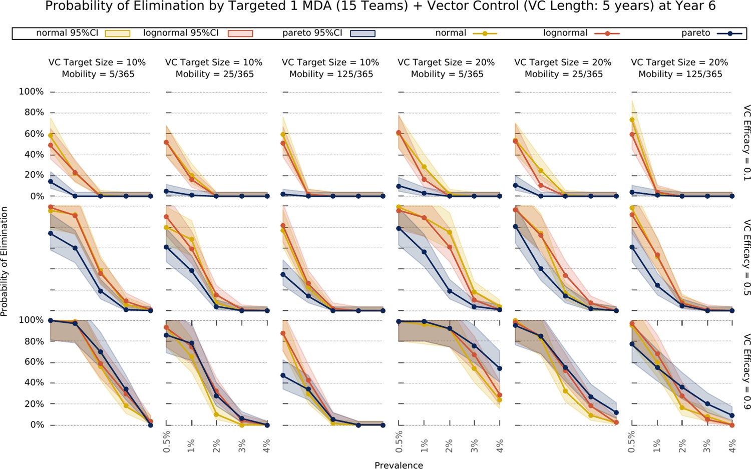
Elimination probability with a targeted approach.
The same as in Figure 5, except that vector control is extended to last 5 years.
Author response image 1
Tables
Table 1
Factors explored by the model and their respective sets of values.
| Factor | Meaning | Values |
|---|---|---|
| Teams | Number of teams performing prevalence surveys and distributing ACTs simultaneously. Translated into coverage speed in square brackets, that is, the number of days it takes to perform one MDA round in a region of 1000 villages. | 15 [267] 25 [160] 50 [80] 100 [40] 200 [20] 400 [10] |
| Prevalence | Mean initial malaria u-PCR prevalence across all villages. | 0.5, 0.1, 0.15, 0.2, 0.25, 0.3 |
| Resistance | Mean initial proportion of parasites which are artemisinin resistant. | 0.1, 0.2, 0.3 |
| Distribution | Transmission heterogeneity distribution, underlying spatial heterogeneity of malaria transmission, manifested by differential mosquito density distributions. | Gaussian, Log-normal, Pareto |
| Mobility | Describes the intensity of population movement in the general population. Indicates the per person average daily probability of moving to places other than their home village for short-term visits (see Mobility section in the Simulation Protocol). that is a population of individuals whose short-term movement occurs on average 25 times per year (25/365) has a relatively static population with low mobility. | 5/365 25/365 125/365 250/365 |
| Campaigns | The number of MDA Campaigns | 1, 2 |
| Peaks | The number of annual seasonal peaks | 1, 2 |
Table 2
List of parameters used in the model.
| # | Name | Description | Value | Reference |
|---|---|---|---|---|
| 1 | V | Set of villages | |V| = 1000 | |
| 2 | N | Set of individuals across all villages | |N| = 314,795 | - |
| 3 | ml | Proportion of males in the population | 0.48 | (National Institute of Statistics, 2008) |
| 4 | maxage | Maximum age | 80 years | - |
| 5 | beta | Biting rate | variable* | - |
| 6 | previ | Initial proportion of infectious people | variable* | - |
| 7 | resit | Initial proportion of artemisinin resistant infections | variable* | - |
| 8 | netuse | Proportion of individuals that own an insecticide treated bed net | 0.5 | - |
| 9 | itneffect | proportional decrease of individual susceptibility/infectiousness related to ITN usage | 0.2 | - |
| 10 | ovstay | Mean number of nights spent somewhere when undertaking short-term population movement | 3 | - |
| 11 | crit | Critical distance below which overnight stays somewhere other than your home are made very unlikely | 4 km | - |
| 12 | timecomp | Mean time to complete ACT routine treatment | 4 days | Best guess |
| 13 | fullcourse | Proportion that receives treatment full course | 0.8 | (Yeung et al., 2008) |
| 14 | covab | Proportion of symptomatic cases that receive antimalarials | 0.6 | (Yeung et al., 2008) |
| 15 | nomp | Relative probability of receiving treatment in a non-malaria post village | 0.1 | Best guess |
| 16 | asymtreat | Relative probability of receiving treatment without clinical symptom | 10−4 | - |
| 17 | tauab | Daily probability of receiving ACT in a village under MDA | 1/1.5 | - |
| 18 | gamma | Mean liver stage duration | 5 days | (Collins and Jeffery, 1999; Eyles and Young, 1951) |
| 19 | sigma | Mean time to infectiousness after liver emergence | 15 days | (Jeffery and Eyles, 1955) |
| 20 | mellow | Mean duration of symptoms | 3 days | (Church et al., 1997) |
| 21 | xa0 | Daily probability of going below the minimum effective artemisinin concentration | 1/7 | (Karbwang et al., 1998) |
| 22 | xai | Daily probability losing the DHA effect as part of ACT | 1/3 | (Rijken et al., 2011; Tarning et al., 2008) |
| 23 | xab | Daily probability of going below the minimum effective piperaquine concentration | 1/30 | (Rijken et al., 2011; Tarning et al., 2008) |
| 24 | xpr | Daily probability of going below the minimum effective primaquine concentration | 1/2 | (Burgess and Bray, 1961) |
| 25 | delta | Mean duration of a malaria untreated infection | 160 days | (Eyles and Young, 1951; Babiker et al., 1998; Franks et al., 2001) |
| 26 | imm_min | Minimum clinical immunity period | 40 days | Best guess |
| 27 | alpha | Average permanence in each immunity level | 60 days | - |
| 28 | phic | Relative infectiousness of symptomatic infections compared to sub-patent ones | 1 | - |
| 29 | mdi | Mosquito daily probability of dying while infectious | 1/7 | (Dawes et al., 2009) |
| 30 | mdn | Mosquito daily probability of dying while infected but not yet infectious | 1/20 | (Dawes et al., 2009) |
| 31 | mgamma | Mean extrinsic incubation period | 14 days | (Smith et al., 2014) |
| 32 | amp | Amplitude of mosquito density seasonal variation | 0.6 | Best guess |
| 33 | process | Days needed to administer a full ACT course in one village | 4 days | Optimistic guess |
| 34 | rounds | Number of drug rounds in an MDA campaign | 3 | Standard practice |
| 35 | btrounds | Number of days between drug rounds in an MDA campaign | 32 | Standard practice |
| 36 | vcefficacy | Vector control efficacy | variable* | - |
| 37 | Daily probability of clearing blood stage drug sensitive parasites with circulating dha | 1/5 | (Adjuik et al., 2004; Pukrittayakamee et al., 2004) | |
| 38 | Daily probability of clearing blood stage artemisinin resistant parasites with dha | 0.27* (0.05) | (Dondorp et al., 2009) | |
| 39 | Daily probability of clearing infectious stage drug sensitive parasites with circulating dha | 1/3 | (Adjuik et al., 2004; Pukrittayakamee et al., 2004) | |
| 40 | Daily probability of clearing infectious stage artemisinin resistant parasites with dha | 0.27* (0.09) | (Dondorp et al., 2009) | |
| 41 | Daily probability of clearing blood stage drug sensitive parasites with circulating dha- piperaquine | 1/3 | (Adjuik et al., 2004; Pukrittayakamee et al., 2004) | |
| 42 | Daily probability of clearing blood stage artemisinin resistant parasites with dha- piperaquine | 0.27* + (1.0–0.27)* (0.33) | (Dondorp et al., 2009) | |
| 43 | Daily probability of clearing infectious stage drug sensitive parasites with circulating dha- piperaquine | 1/3 | (Bustos et al., 2013) | |
| 44 | Daily probability of clearing infectious stage artemisinin resistant parasites with dha- piperaquine | 0.27* + (1.0–0.27)* (0.126) | - | |
| 45 | Daily probability of clearing blood stage drug sensitive parasites with circulating piperaquine | 1/3 | (Chen et al., 1982) | |
| 46 | Daily probability of clearing blood stage artemisinin resistant parasites with piperaquine | 1/3 | (Chen et al., 1982) | |
| 47 | Daily probability of clearing infectious stage drug sensitive parasites with circulating piperaquine | 1/20 | (Myint et al., 2007) | |
| 48 | Daily probability of clearing infectious stage artemisinin resistant parasites with piperaquine | 1/20 | (Myint et al., 2007) | |
| 49 | Daily probability of clearing infectious stage drug sensitive parasites with primaquine | 1/1.5 | (Burgess and Bray, 1961; Smithuis et al., 2010) | |
| 50 | Daily probability of clearing infectious stage artemisinin resistant parasites with primaquine | 1/1.5 | - | |
| 51 | k | Steepness of susceptibility increase with age | 0.14 | (Aguas et al., 2008) |
| 52 | r | Amplitude of susceptibility increase with age | 0.99 | (Aguas et al., 2008) |
-
*the values are varied in different simulation settings. Their values are given in the description of each set of experiments and the set of possible values is given in Table 1.
Additional files
Download links
A two-part list of links to download the article, or parts of the article, in various formats.
Downloads (link to download the article as PDF)
Open citations (links to open the citations from this article in various online reference manager services)
Cite this article (links to download the citations from this article in formats compatible with various reference manager tools)
Determinants of MDA impact and designing MDAs towards malaria elimination
eLife 9:e51773.
https://doi.org/10.7554/eLife.51773


