Spatiotemporal patterns of neocortical activity around hippocampal sharp-wave ripples
- Canadian Centre for Behavioral Neuroscience, University of Lethbridge, Canada
- Department of Electrical Engineering and Computer Science, University of California, United States
- Medical Scientist Training Program, University of California, United States
- Department of Neurobiology and Behavior, University of California, United States
Figures
Figure 1 with 4 supplements
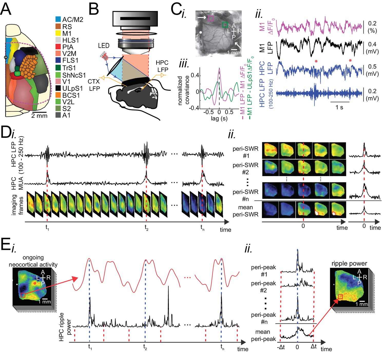
Experimental protocol for investigating dynamics of neocortical-hippocampal interactions during sleep.
(A) Schematic of a cranial window for wide-field optical imaging of neocortical activity using voltage or glutamate probes. The voltage or glutamate signal was recorded from dorsal surface of the right neocortical hemisphere, containing the specified regions. The red dashed line marks the boundary of a typical cranial window. The abbreviations denote the following cortices AC/M2: anterior cingulate/secondary Motor, RS: retrosplenial, M1: primary motor, HLS1: hindlimb primary somatosensory, PtA: posterior parietal, V2M: secondary medial visual, FLS1: forelimb primary somatosensory, TrS1: trunk primary somatosensory, ShNcS1: shoulder/neck primary somatosensory, V1: primary visual, ULpS1: lip primary somatosensory, BCS1: primary barrel, V2L: secondary lateral visual, S2: secondary somatosensory, A1: primary auditory. (B) Schematic of the experimental setup for simultaneous electrophysiology and wide-field optical imaging. A CCD camera detects reflected light coming from fluorescent indicators, in the superficial neocortical layers, which are excited by the red or blue LEDs. An additional infra-red camera recorded pupil diameter (not shown). Hippocampal LFP recordings were conducted for SWR and MUA detection. A neocortical LFP recording was also acquired to compare imaging and electrophysiological signals. (C) (i) Photomicrograph of the wide unilateral craniotomy with bregma indicated by a white circle in each image. Compass arrows indicate anterior (A), posterior (P), medial (M) and lateral (L) directions. The white arrow indicates a neocortical LFP electrode position. (ii) Exemplar voltage signal recorded from a region in the M1 indicated by a magenta square in Ci, aligned with neocortical and hippocampal LFPs, and a hippocampal trace filtered in the ripple band. Asterisks indicate detected SWRs. (D) Schematic figure demonstrating the peri-SWR averaging of neocortical activity. (i) Ripple band filtered LFP trace displaying three example SWRs (top row) and hippocampal multi-unit activity (MUA) trace (middle row), temporally aligned with concurrently recorded neocortical voltage activity (bottom row). (ii) For each detected SWR, corresponding neocortical imaging frames (left rows) and MUA traces (right rows) are aligned with respect to SWR centers and then averaged (bottom rows). (E) Demonstration of how peri-neocortical-peak-activation average ripple power was calculated. (i) The red trace is the voltage signal from the indicated region of interest (red square) shown in the image on the left. The black trace is the temporally aligned hippocampal ripple power time series. Blue dashed lines are the timestamps of three detected peak activations in the indicated neocortical region. (ii) For each detected peak activation, ripple power traces were aligned and averaged. This figure has two figure supplements.
Figure 1—figure supplement 1
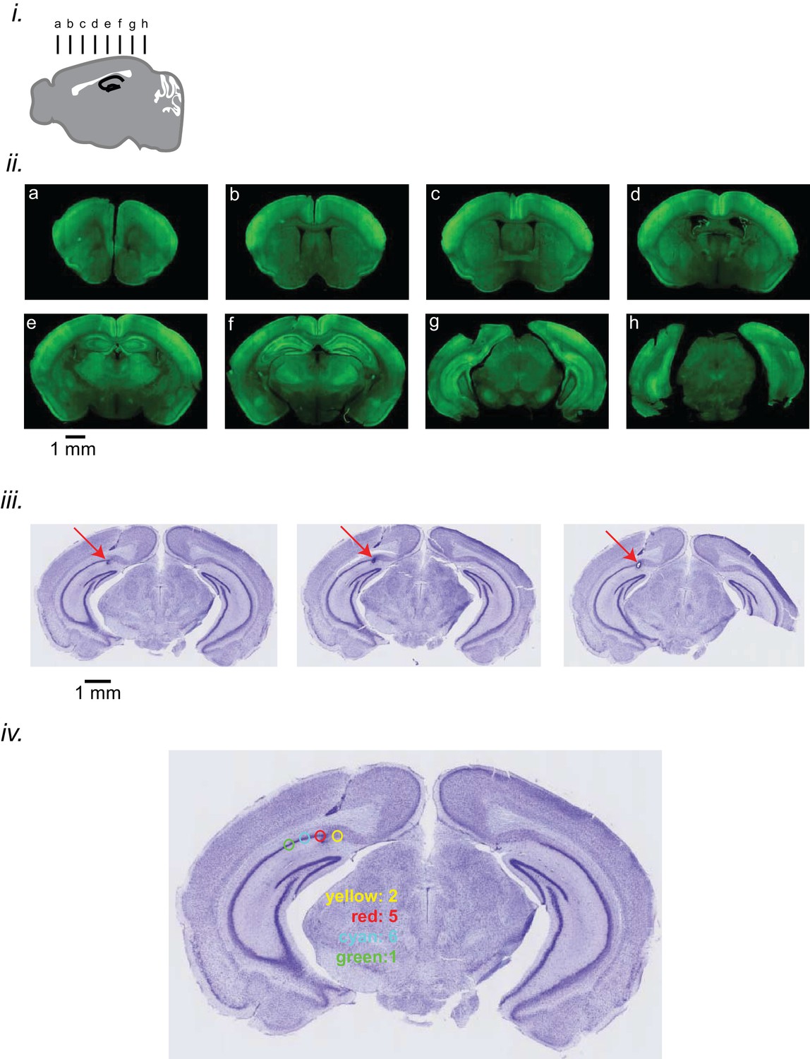
Expression level of iGluSnFR and electrode localization.
(i) Schematic diagram representing the location of coronal sections presented here. (ii) Coronal sections showing the expression of iGluSnFR in the neocortex and hippocampus in EMX-CaMKII-Ai85 mouse. (iii) Coronal sections of the brain of a representative animal, stained with Nissl, showing the location of the tip of the hippocampal LFP electrode in the pyramidal layer of the CA1 subfield of the hippocampus. The sections are ordered from anterior to posterior from left to right. (iv) The distribution of HPC LFP electrode tips in 14 mouse brains is represented. The location of tips is categorized into 4 groups, each of which is colored differently. The number of animals in each colored category is reported on the figure.
Figure 1—figure supplement 2
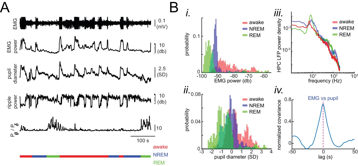
Physiological signatures of different brain states in the head-restrained mouse.
(A) Representative traces of local field potentials (LFP) and electromyography (EMG) during waking, NREM and REM sleep. From top to bottom: raw EMG signal, EMG power measured at 30–1000 HZ, pupil diameter, hippocampal ripple power, theta-to-delta band power ratio trace calculated from hippocampal LFP signal, and hypnogram. In the hypnogram, REM, NREM, and awake represent states of animals i.e. REM sleep, NREM sleep, and wake periods, respectively, which were scored from EMG traces and hippocampal LFPs theta-to-delta band ratio. The EMG raw signal values are clipped for visualization purposes but the true values were used for scoring the sleep/wake period. (B) Histograms in (i) and (ii) show the distribution of EMG power and z-scored pupil diameter in a representative recording session across waking, NREM and REM sleep. Note the segregation of histograms across brain states. (iii) Exemplar hippocampal LFP power spectral density calculated for the same three states in a representative recording session. (iv) Representative normalized cross-covariance between EMG power and pupil diameter signals, showing a strong correlation at zero lag.
Figure 1—video 1
Spontaneous neocortical voltage activity with concurrently recorded hippocampal LFP and ripple activity.
Example of neocortical spontaneous voltage activity captured by voltage-sensitive dye imaging under urethane anesthesia and filtered in 0.5–6 Hz band. The blue traces are concurrently recorded hippocampal local field potential filtered in two frequency bands: 0.1–1000 Hz (middle) and 100–250 Hz (bottom).
Figure 1—video 2
Wake/sleep scoring.
Example of the physiological signals used for wake/sleep scoring recorded during a transition from awake state to NREM and then REM sleep. Notice the lack of any movement during NREM and the facial muscle twitches during REM sleep.
Figure 2 with 8 supplements
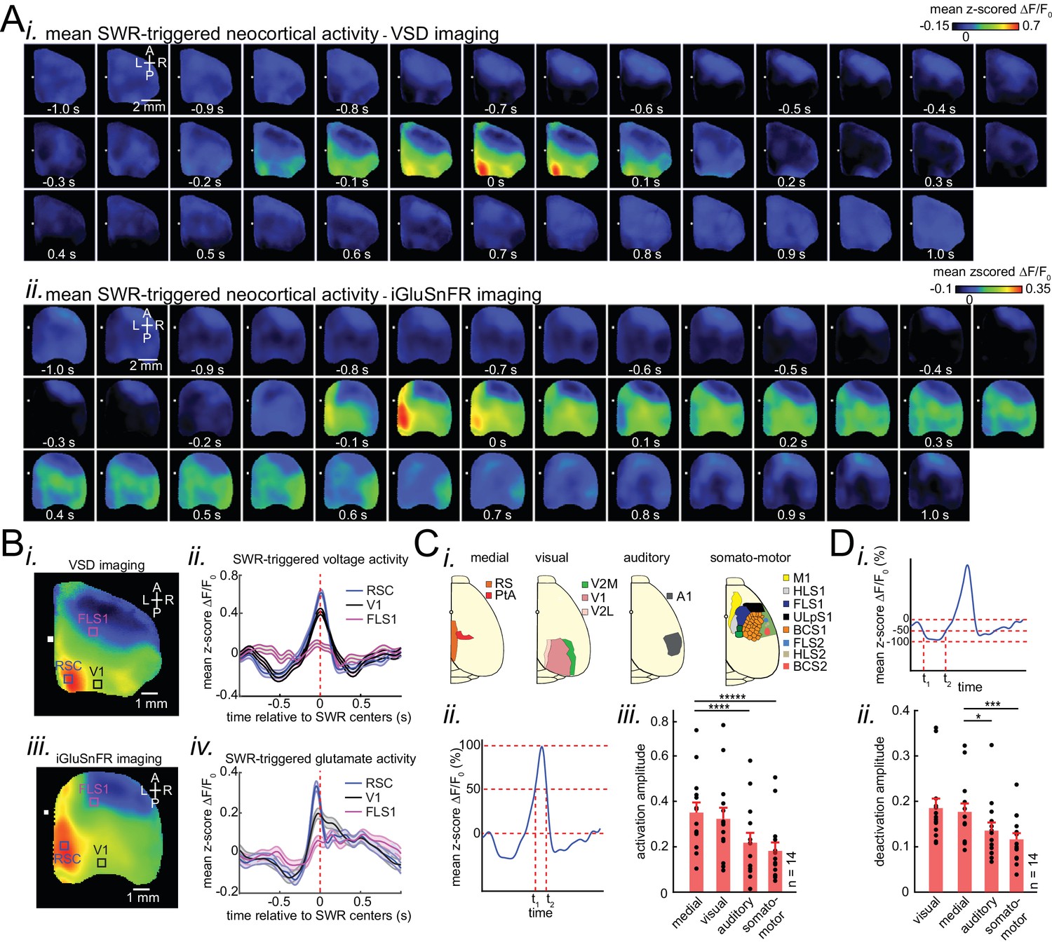
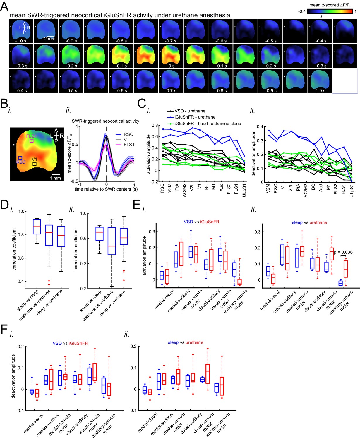
Patterns of activity in neocortical regions are differentially modulated around hippocampal SWRs.
(A) Representative montage of mean peri-SWR neocortical activity measured using (i) voltage-sensitive dye and (ii) glutamate-sensing fluorescent reporter iGluSnFR under urethane anesthesia and head-restrained natural sleep, respectively. 0s-time indicates SWR centers. Images have been z-scored and scaled to the depicted color bars. (B) (i–iv) Example traces showing voltage or iGluSnFR signals from selected regions in (i) and (iii). Plots are the average of optical signals measured from 3 × 3 pixel boxes (~0.04 mm2) placed within retrosplenial (blue), visual (black), and forelimb somatosensory (magenta) cortices. The thickness of the shading around each plot indicates SEM. 0 s-time indicates SWR centers. (C) (i) Four major structurally defined neocortical subnetworks (medial, visual, auditory and somato-motor). (ii) Demonstration of how the activation amplitudes were quantified. The activation amplitude was defined as the mean of the signal across full-width at half maximum (t1 to t2). (iii) Grand average (n = 14 animals) of activation amplitudes across neocortical subnetworks, sorted in decreasing order. Each data point is the average of activation amplitudes of all regions in a given subnetwork and in a given animal. (repeated measure ANOVA with Greenhouse-Geisser correction for sphericity: F3,39 = 44.303, p=2.2193 × 10⁻¹⁰; post-hoc multiple comparison with Tuckey’s correction: medial vs visual p=0.11844, medial vs auditory p=7.8147 × 10⁻⁵, medial vs somatomotor p=1.1128 × 10⁻⁶, visual vs auditory p=0.00024702, visual vs somatomotor p=2.9247 × 10−05, auditory vs somatomotor p=0.19802) (D) (i–ii) Same measurements as in C, but for neocortical deactivations preceding SWRs. Note that the deactivation peaks were rectified for group comparison in (ii). A higher value of deactivation amplitude indicates stronger deactivation. Bar graphs indicate mean ± SEM. (repeated measure ANOVA with Greenhouse-Geisser correction for sphericity: F3,39 = 15.508, p=1.1009 × 10⁻⁵; post-hoc multiple comparison with Tuckey’s correction: medial vs visual p=0.63021, medial vs auditory p=0.014438, medial vs somatomotor p=0.00076384, visual vs auditory p=0.0042707, visual vs somatomotor p=0.0014657, auditory vs somatomotor p=0.5317). This figure has five figure supplements.
-
Figure 2—source data 1
Differential activation amplitude across neocortical subnetworks around SWRs.
- https://cdn.elifesciences.org/articles/51972/elife-51972-fig2-data1-v3.mat
-
Figure 2—source data 2
Differential deactivation amplitude across neocortical subnetworks around SWRs.
- https://cdn.elifesciences.org/articles/51972/elife-51972-fig2-data2-v3.mat
Figure 2—figure supplement 1

Representative spatiotemporal patters of neocortical activity around hippocampal SWRs.
Neocortical activity centered (t = 0) on three randomly selected individual SWRs is represented.
Figure 2—figure supplement 2

Characteristics of SWRs recorded in urethane anesthesia, head-restrained and unrestrained naturally sleeping mice.
(A) Exemplar HPC LFP signals recorded under urethane anesthesia (i) and natural sleep (ii). (B) (i) Median peak spectral frequency of hippocampal SWRs recorded under different experimental conditions: urethane anesthesia, head-restrained sleep, and unrestrained sleep. C57BL/6 mice were used in experiments in which the animals were either anesthetized with urethane for VSD imaging or unrestrained and naturally sleeping. EMX-CaMKII-Ai85 mice were imaged during head-restrained sleep or under urethane anesthesia. Each data point is the median value in a given animal. SWRs detected under urethane anesthesia tend to have slower peak frequencies. The red plus signs represent the data points outside the interval (centered on median value) which includes 99.3 percent of all data points. (ii) Similar to (i) but the histograms here is showing the distribution of peak spectral frequency of hippocampal SWRs pooled across all animals and across experimental conditions. (C–D) (i,ii) similar to A, duration (width) and inter-SWR time intervals of hippocampal SWRs are represented under different experimental conditions. Note that the SWRs detected under urethane anesthesia tend to have shorter durations. (E) The same as C (ii) but the histograms are plotted in the logarithmic scale.
Figure 2—figure supplement 3
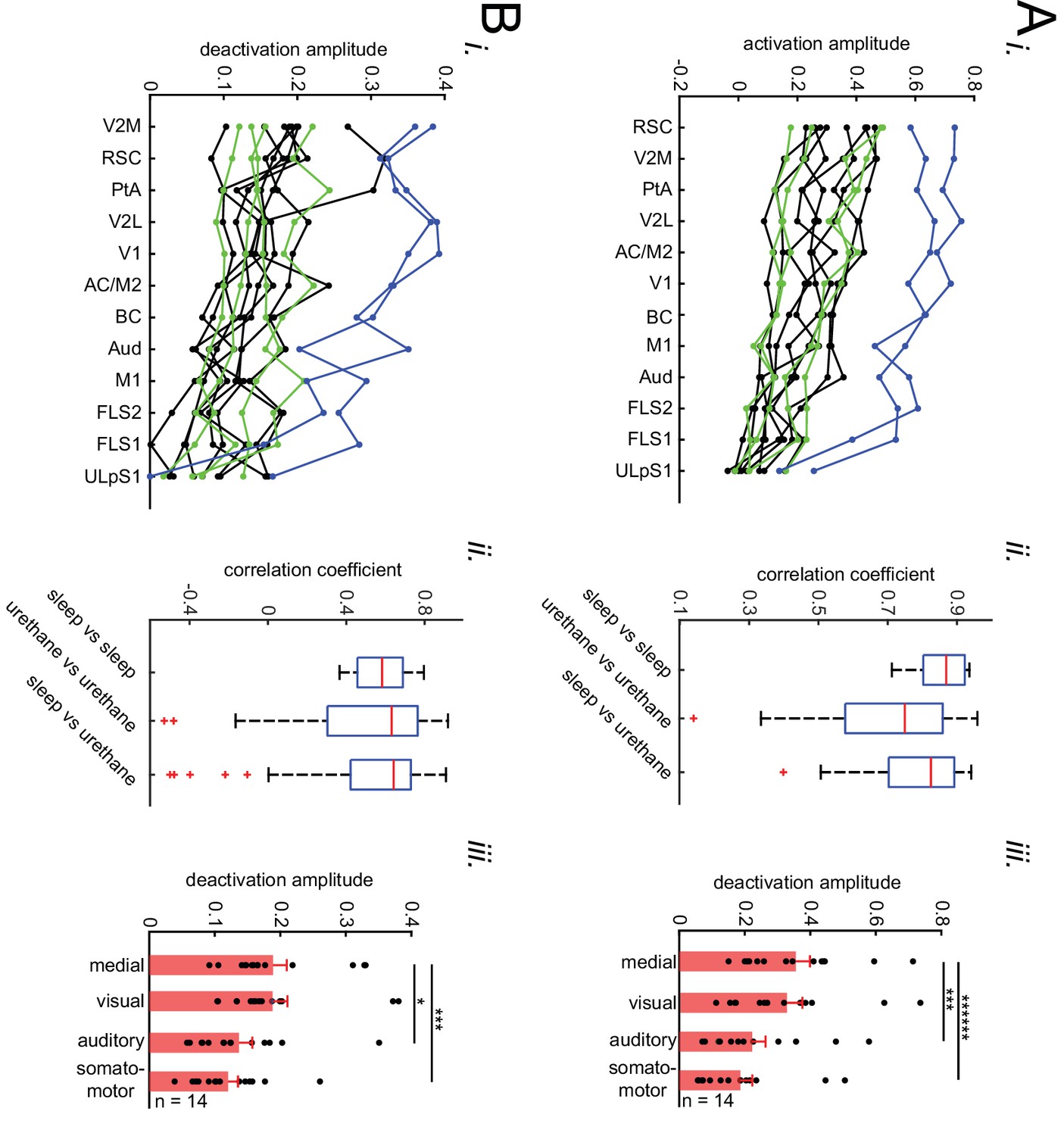
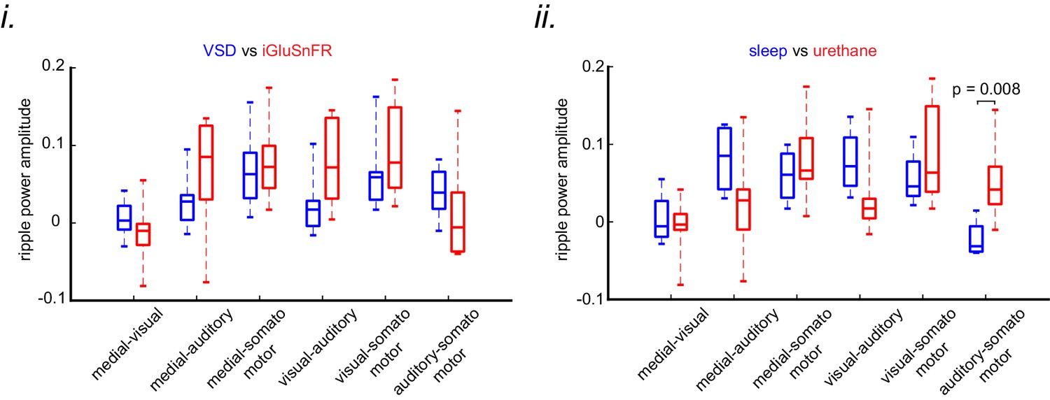
Differential modulation of neocortical regions under sleep/urethane anesthesia and VSD/iGluSnFR imaging conditions are similar.
(A) Representative mean peri-SWR neocortical activity (0-time indicates SWR centers) recorded in urethane-anesthetized EMX-CaMKII-Ai85 mice. This animal was also recorded under natural sleep (see Figure 2A ii). Mean peri-SWR neocortical activity patterns during head-restrained sleep are similar to spatiotemporal patterns of neocortical deactivation and activation around SWR times obtained under urethane-anesthesia. (B) Plots are the average of the iGluSnFr signals measured from 3 × 3 pixel boxes (~0.04 mm2) placed within retrosplenial (blue trace), visual (black trace), and forelimb somatosensory (magenta trace) cortices. The thickness of the shading around each plot indicates SEM. Time-series representation of peri-SWR neocortical activity allows for better visualization of temporal differences in activation of different regions. (C) Peri-SWR activation (i) and deactivation (ii) amplitudes across distinct neocortical regions, sorted in decreasing order. Each piece-wise linear trace is associated with a particular animal (n = 14 mice). These data were used to generate bar graphs presented in Figure 2C iii and 2D ii by averaging the data points across regions in a given neocortical structural subnetwork. The color code represents different recording conditions. (D) Quantification of similarities between the trends of activation (i) and deactivation (ii) amplitudes across neocortical regions under urethane anesthesia and natural sleep. The box plot shows the distribution of correlation coefficients between all possible pairs of traces associated with natural sleep (green lines in C) and urethane anesthesia (blue and black lines in C). Horizontal red lines represent the median of each distribution. As measured by correlation coefficients, there is no significant difference between both activation and deactivation amplitude trends under urethane anesthesia and natural sleep. Therefore, we decided to pool the urethane and natural sleep data in this paper. The red plus signs represent the data points outside the interval (centered on median value) which includes 99.3 percent of all data points. (E) The difference of activation amplitudes (arithmetic subtraction) between all possible pairs of subnetworks is compared across VSD versus iGluSnFR (i) and sleep versus urethane conditions (ii). The only statistically significant result is from the difference auditory-somatosensory (auditory minus somatosensory) in sleep versus urethane comparison. (F) The same as E but for deactivation amplitude. There was no significant statistical difference across conditions.
Figure 2—figure supplement 4
Differential modulation of neocortical regions does not depend on SWR detection threshold value.
(A) (i) Peri-SWR activation amplitudes across neocortical regions sorted in the descending order. Each piece-wise linear curve connecting the activation amplitudes of neocortical regions is associated with a particular animal (n = 14). These data were generated using a higher SWR detection threshold (mean plus 3 (VSD) or 4 (iGluSnFR) times standard deviation of the ripple power signal) compared to that used to generate data presented in Figure 2 and Figure 2—figure supplement 2 (mean plus 2 (VSD) or 3 (iGluSnFR) times standard deviation of the ripple power signal). (ii) Quantification of similarities between trends of peri-SWR activation amplitudes across neocortical regions under urethane anesthesia and natural sleep. The box plot shows the distribution of correlation coefficients between all possible pairs of traces associated with natural sleep (green lines in i) and urethane anesthesia (blue and black lines in i). The Horizontal red lines represent the median of each distribution. As measured by correlation coefficients, there is no significant difference between peri-SWR activation amplitude trends under urethane anesthesia and natural sleep. (iii) Grand average (n = 14 animals) of peri-SWR activation amplitudes across neocortical subnetworks, sorted in decreasing activation amplitude. Each data point is the average of the activation amplitudes of all regions in a given subnetwork. (B) The same as in A but for peri-SWR deactivation amplitudes.
Figure 2—figure supplement 5
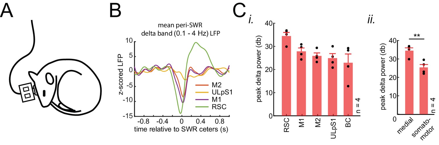
Differential modulation of neocortical activity, measured by LFP, around SWRs.
(A) Schematic of electrophysiological recordings in naturally sleeping mice. (B) Example traces of mean peri-SWR neocortical LFP signals obtained during sleep. The neocortical LFP activity were filtered in delta band (0.1–4 Hz) across four neocortical regions including retrosplenial cortex (RCS), Primary and secondary motor cortex (M1 and M2), and upper lip somatosensory cortex (ULpS1). LFP filtered signal was z-scored with respect to a distribution of traces for each region, triggered around random timestamps generated by shuffling inter-SWR intervals. RSC, on average, shows the largest negative deflection (activation) and earliest onset around ripples times (0 s). (C) (i) Group average (n = 4 animals) of delta-band peak power across neocortical regions, sorted in descending order. Z-scored delta power is reported in the logarithmic scale (decibels, db). RSC shows the largest delta power across all regions and animals. (ii) Grouping the data from four neocortical regions into neocortical subnetworks, defined in Figure 2C i, shows that medial subnetwork compared to the somatomotor subnetwork receive stronger modulation around hippocampal SWRs (p<0.01, one-sided Wilcoxon signed-rank test).
Figure 2—video 1
Mean peri-SWR voltage activity under urethane anesthesia.
Example of mean peri-SWR voltage activity captured by voltage-sensitive dye imaging under urethane anesthesia. The voltage signal is filtered in 0.5–6 Hz band. The blue trace represents the mean peri-SWR hippocampal LFP.
Figure 2—video 2
Mean peri-SWR iGluSnFR activity during head-restrained sleep anesthesia.
Example of mean peri-SWR extracellular glutamate activity captured by iGluSnFR imaging during head-restrained sleep. The iGluSnFR signal is filtered in 0.5–6 Hz band. The blue trace represents the mean peri-SWR hippocampal LFP.
Figure 2—video 3
Mean peri-SWR iGluSnFR activity under urethane anesthesia.
Example of mean peri-SWR extracellular glutamate activity captured by iGluSnFR imaging under urethane anesthesia. The iGluSnFR signal is filtered in 0.5–6 Hz band. The blue trace represents the mean peri-SWR hippocampal LFP.
Figure 3 with 2 supplements
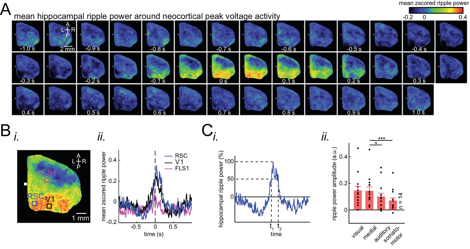
Ripple power is distinctively correlated with peak activity in different neocortical subnetworks.
(A) Representative montage (50 ms intervals) showing spatiotemporal pattern of mean hippocampal ripple power fluctuations around the peak of neocortical activations. 0s-time indicates peak activation time in each neocortical pixel. Color bar represents the mean z-scored ripple power associated with peak activation in a given neocortical pixel. (B) (i–ii) A representative frame showing the spatial distribution of ripple power at neocortical peak activation time. Colored squares represent three regions of interest (retrosplenial, visual, and forelimb somatosensory cortices in blue, black and magenta, respectively) for which their associated ripple power traces are displayed in (ii). (C) (i) Illustration of how the ripple power amplitude was quantified. Ripple power amplitude was defined as the mean ripple power signal across full-width at half maximum (t1 to t2). (ii) Grand average (n = 14 animals) of mean hippocampal ripple power amplitudes across neocortical subnetworks shown in Figure 2Ci, sorted in decreasing order. Each data point is the average of hippocampal ripple power amplitudes associated with all the regions in a given subnetwork and in a given animal. Bar graphs indicate mean ± SEM. (repeated measure ANOVA with Greenhouse-Geisser correction for sphericity: F3,39 = 14.172, p=1.8183 × 10⁻⁵; post-hoc multiple comparison with Tuckey’s correction: medial vs visual p=0.99476, medial vs auditory p=0.073032 [p=0.0152 without Greenhouse-Geisser correction], medial vs somatomotor p=0.00054029, visual vs auditory p=0.030248, visual vs somatomotor p=0.0010466, auditory vs somatomotor p=0.17794). This figure has two figure supplements.
-
Figure 3—source data 1
Correspondence of ripple power with peak activity in different neocortical subnetworks.
- https://cdn.elifesciences.org/articles/51972/elife-51972-fig3-data1-v3.mat
Figure 3—figure supplement 1
The correlation of ripple power with neocortical peak activity is similar under sleep/urethane anesthesia and VSD/iGluSnFR imaging conditions.
The difference of ripple power amplitudes (arithmetic subtraction) between all possible pairs of subnetworks is compared across VSD versus iGluSnFR (i) and sleep versus urethane anesthesia (ii) conditions. The only statistically significant result is from the difference auditory-somatosensory (auditory minus somatosensory) in sleep versus urethane comparison.
Figure 3—figure supplement 2
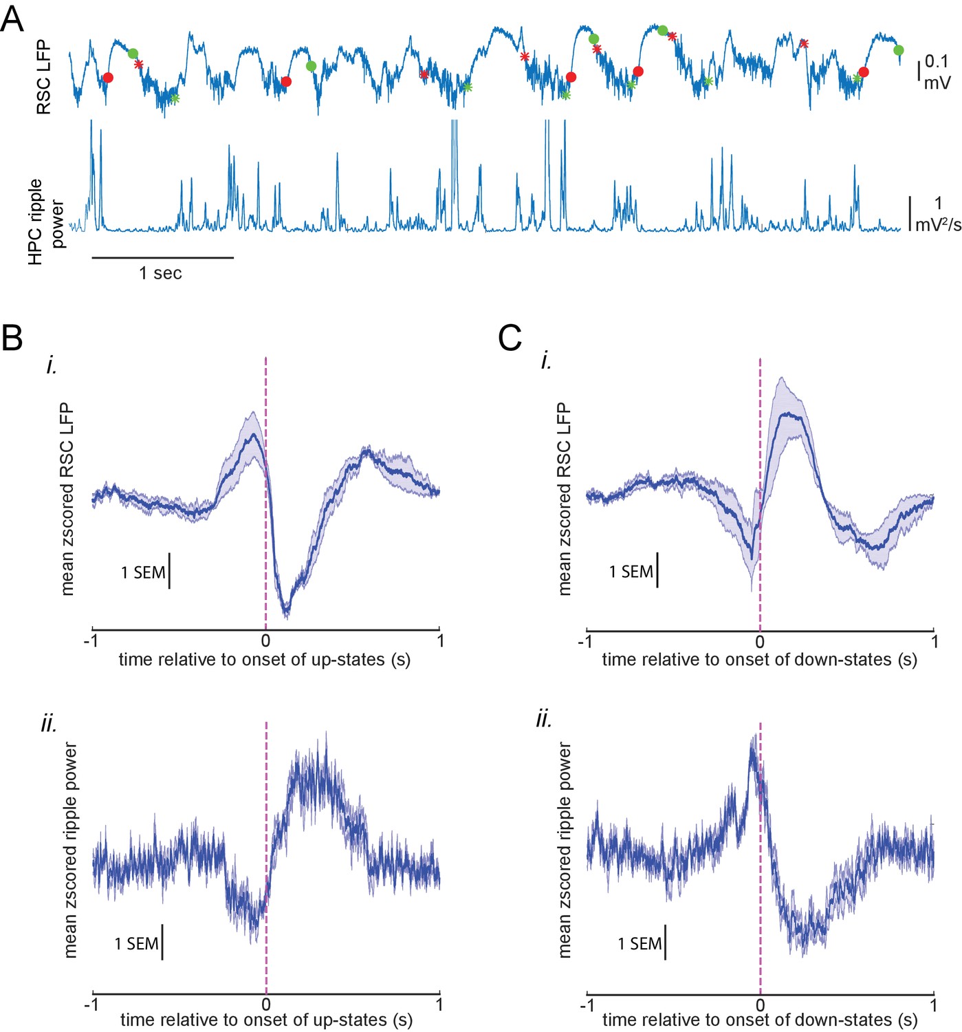
Modulation of hippocampal ripple power around neocortical up-/down-states.
(A) Exemplar LFP signals recorded with a bipolar electrode from the retrosplenial cortex (RSC; top) and dorsal CA1 of the hippocampus (filtered in ripple band, rectified, and smoothed; bottom) during slow oscillation. Red and green circles represent the onset and offset of detected RSC down-states, respectively. Similarly, red and green stars represent the onset and offset of detected RSC up-states, respectively. (B) Mean z-scored RSC LFP (i) and ripple power (ii) traces aligned to the onset of RSC up-states. The shaded area represents the SEM (n = 4 animals). Notice that the ripple power is suppressed and elevated before and after the onset of up-states, respectively. (C) Mean z-scored RSC LFP (i) and ripple power (ii) traces aligned to the onset of RSC down-states. The shaded area represents the SEM (n = 4 animals). Notice that the ripple power is elevated and suppressed before and after the onset of down-states, respectively.
Figure 4 with 2 supplements
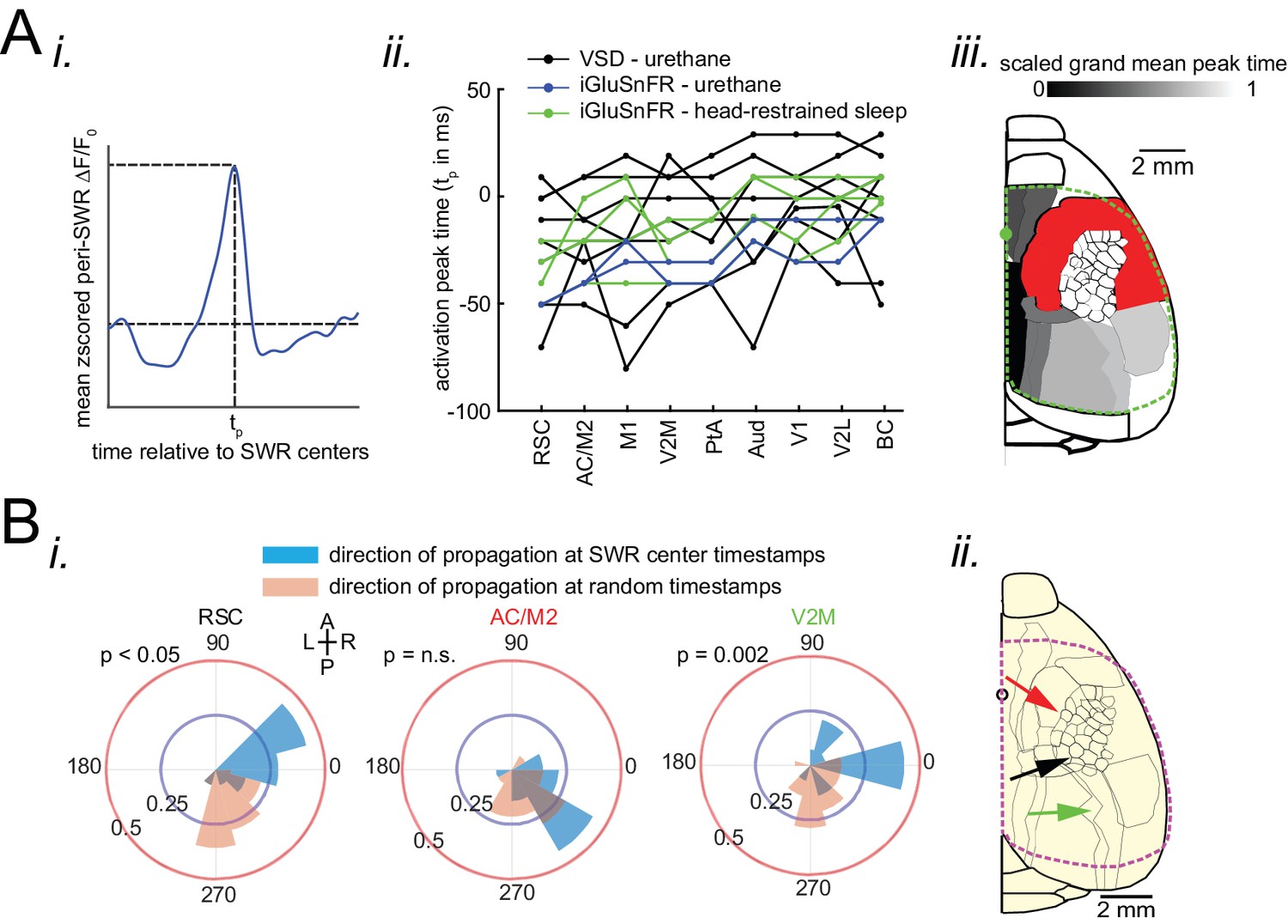
Neocortex tends to sequentially activate from medial to more lateral regions around SWRs.
(A) (i) Demonstration of how peri-SWR neocortical activation peak time (tp) was quantified. The mean peri-SWR neocortical activity trace was generated for each region (blue trace) and the timestamp of the peak was defined as tp. (ii) Peri-SWR activation peak timestamp (tp) relative to SWR centers (0s-time) across neocortical regions sorted in ascending order. Each line graph represents one animal. tp values were not detected in some regions and in some animals (three data points in total), mainly because there was not a strong activation in those regions. Such missing data points were filled by average of available data points in the same region and in other animals (repeated measure ANOVA: F8,104 = 8.357195, p<0.0001; post-hoc test for linear trend: slope = 0.003252024 s/region, p<0.0001). (iii) Spatial map of peri-SWR activation peak time across all animals (n = 14) indicating a medial-to-lateral direction of activation. The red area was not included in this analysis because it was not activated strong enough to yield a reliable result. (B) (i) Circular distributions represent the direction of propagating waves of activity in three distinct neocortical regions at hippocampal SWR (blue distribution) and at random timestamps generated by shuffling inter-SWR time intervals (red distribution). 180–0 and 90–270 degrees represent the medio-lateral and antero-posterior axes, respectively. P-values come from Kuiper two-sample test. (ii) Schematic of propagation directions measured at SWR timestamps in three neocortical regions located in the medial neocortex. This figure has two figure supplement.
Figure 4—figure supplement 1
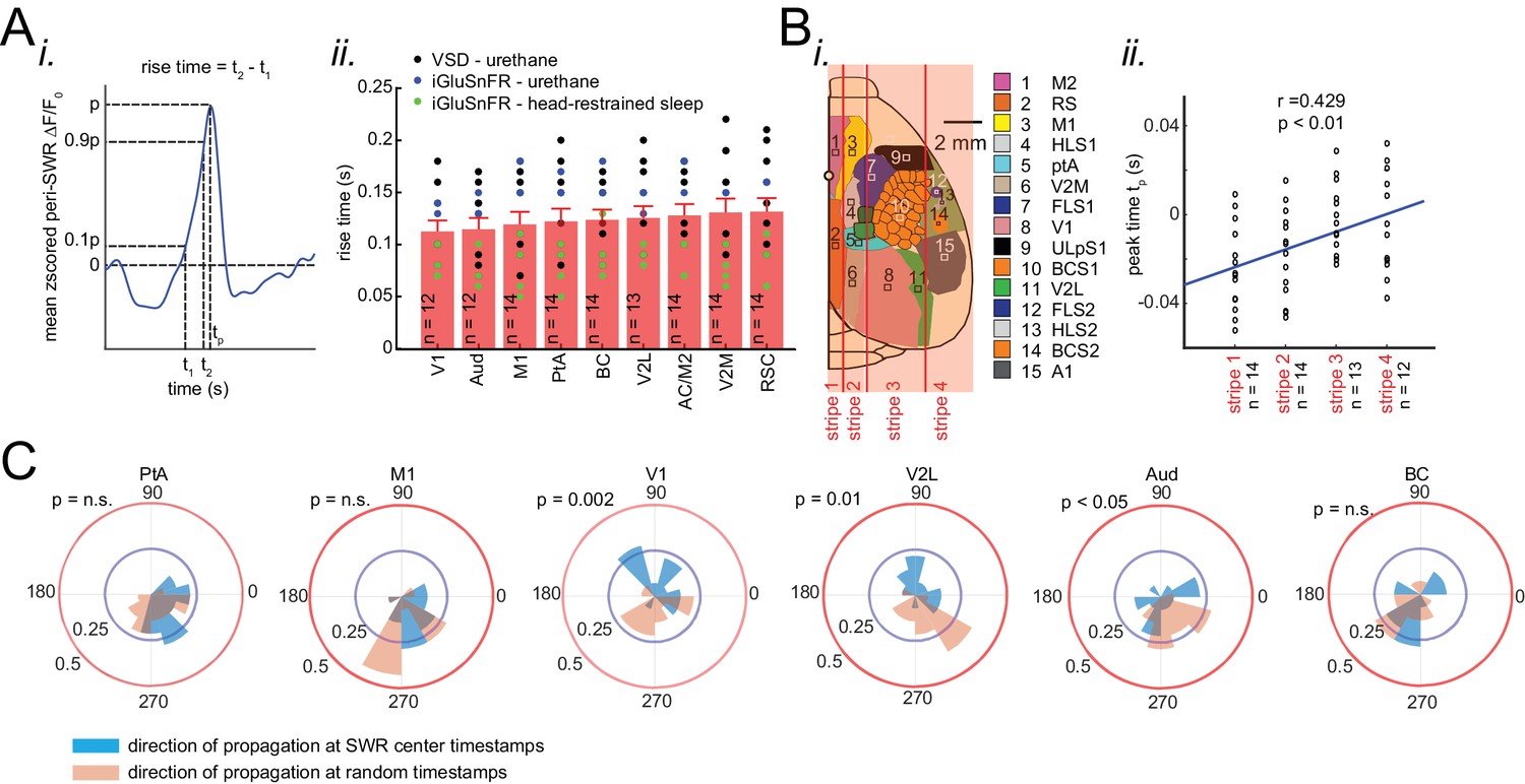
Neocortex tends to activate sequentially from medial to more lateral regions around SWRs.
(A) (i) Demonstration of how peri-SWR neocortical activation rise time was measured. Rise time was calculated as the time which takes for the signal to reach 90% of the peak value starting from 10%. (ii) Summary of the mean peri-SWR activation rise time across neocortical regions from n = 12–14 mice imaged during states of urethane anesthesia (blue and black dots) and head-restrained sleep (green dots). There is no significant difference in activation rise time across neocortical regions meaning that all imaged neocortical regions activate at the same rate. It suggests that activation peak time can reflect the activation time of a given region. The bar graphs are mean ± SEM. (B) Schematic representation of vertical stripes splitting the recorded neocortical regions from medial to lateral into four groups. (ii) There is a significant correlation (r = 0.429, p<0.01, two-sided t-test) between stripe number and peak activation timestamp (tp) indicating that the more lateral regions activate later than medial ones relative to hippocampal SWRs. Dots represent the average tp across regions in each stripe and for each animal. (C) Circular distributions represent the direction of neocortical propagating waves of activation in a given region at hippocampal SWR timestamps (blue distribution) and at random timestamps generated by shuffling inter-SWR time intervals (red distribution). 180–0 degrees represent the medio-lateral and 90–270 degrees represent the antero-posterior axes (p-values are calculated based on Kuiper two-sample test).
Figure 4—figure supplement 2
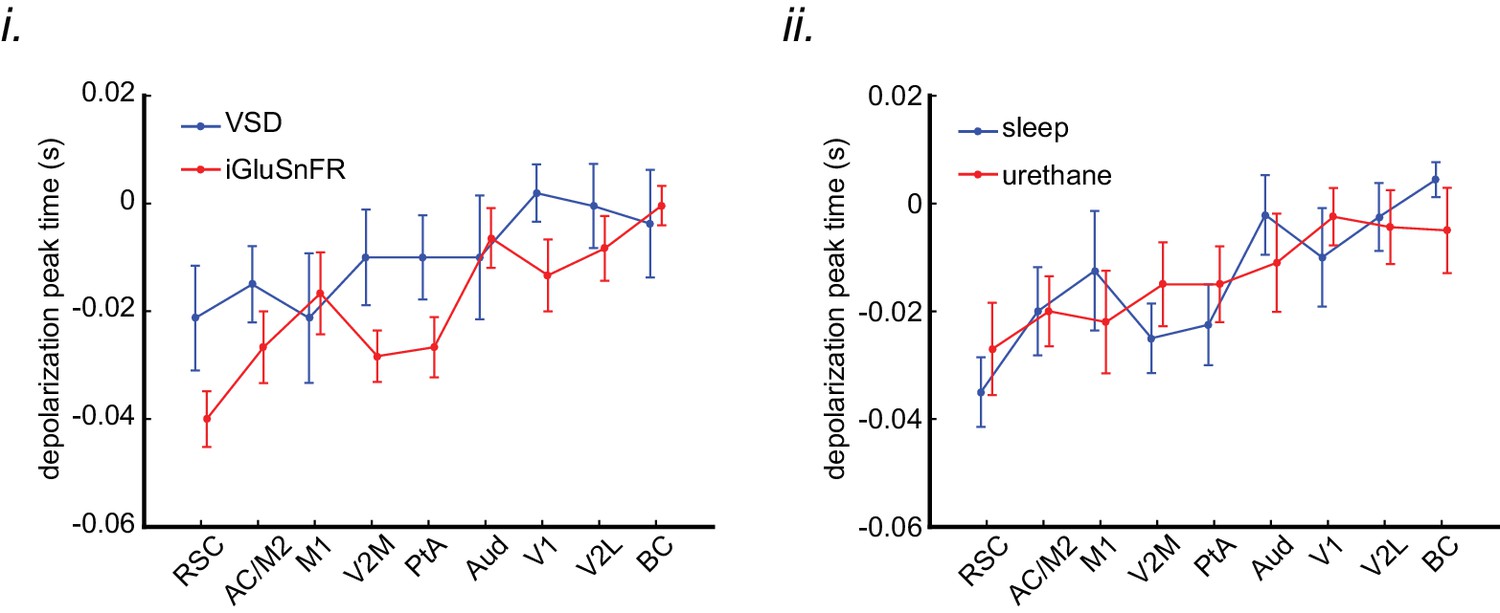
The order of sequential activation across neocortical regions around SWRs is similar under sleep/urethane anesthesia and VSD/iGluSnFR imaging conditions.
The peak time of mean peri-SWR activation across neocortical regions is displayed for VSD versus iGluSnFR (i) and sleep versus urethane anesthesia (ii) conditions. The regions on the horizontal axes are sorted in an increasing order based on the average of all animals (n = 14) in each region. The linear trend in all the four conditions are statistically significant (repeated measure ANOVA follow-up test for linear trend; VSD: slope = 0.002665 s/region, iGluSnFR: slope = 0.004034 s/region, sleep: slope = 0.003968 s/region, and urethane: slope = 0.002966 s/region; All the p-values are less than 0.0001). Error bars represent standard errors.
Figure 5 with 3 supplements
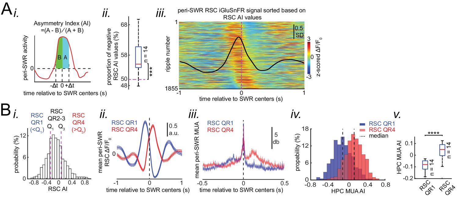
Neocortical activation latency relative to SWRs spans a wide spectrum of negative to positive values.
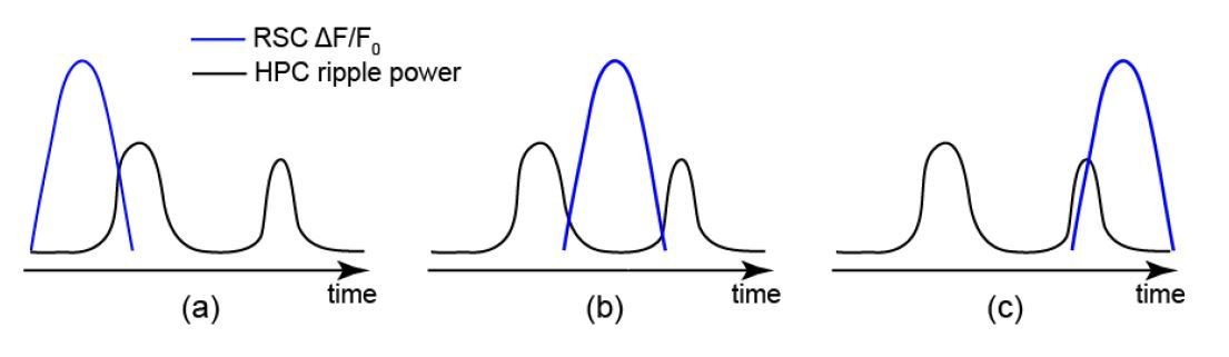
(A) (i) Schematic of Asymmetry Index (AI) calculation. In this figure, AI was calculated for individual peri-SWR retrosplenial cortex (RSC) traces and called RSC AI. RSC AI values were used to quantify the latency of neocortical activation relative to SWR timestamps. (ii) The proportion of negative RSC AI values across animals (n = 14). Magenta dashed line indicates the chance level (50%). 55% (median, indicated by a red line) of peri-SWR RSC activity across animals have negative AI, meaning that on average, neocortical tendency to activate prior to hippocampal SWRs is greater than chance (n = 14; one-sided one-sample Wilcoxon signed-rank test; the median is greater than 0.5 with p=1.831 × 10⁻⁴). (iii) Representative peri-SWR RSC activity sorted by AI calculated for each individual peri-SWR RSC trace. Color bar represents z-scored iGluSnFR signal. The black trace shows the mean peri-SWR RSC iGluSnFR signal. Note that the chance of neocortical activation preceding SWRs is higher than following them. (B) (i) Distribution of RSC AI values for a representative animal. Dashed lines indicate the first (Q1) and third quartiles (Q3). The SWRs for which the associated RSC AI values are less and greater than Q1 and Q3 are called RSC QR1 and QR4, respectively. RSC QR2-3 consists of all other SWRs. (ii) Example plots of mean peri-SWR RSC iGluSnFR signal associated with RSC QR1 (blue) and QR4 (red). The thickness of the shading around each plot indicates SEM. Note that the activity associated with RSC QR1 and QR4 peak before and after SWR centers, respectively. (iii) Time course of exemplar mean peri-SWR hippocampal MUA associated with SWRs in RSC QR1 (blue) and RSC QR4 (red). Notice that both hippocampal MUA activity and RSC iGluSnFR activity are negatively (negative AI) and positively (positive AI) skewed for RSC QR1 and QR4, respectively. (iv) Distributions of hippocampal MUA AI values for SWRs in RSC QR1 (blue) and QR4 (red) in a representative animal. The vertical line represents the median of each distribution. (v) Summary of median values calculated in (iv) across all animals (n = 14, one-sided paired Wilcoxon signed-rank test; RSC QR1 versus RSC QR4 p=6.103 × 10⁻⁵). This figure has three figure supplement.
-
Figure 5—source data 1
Comparing HPC MUA AI median values across RSC QR1 and RSC QR4.
- https://cdn.elifesciences.org/articles/51972/elife-51972-fig5-data1-v3.mat
Figure 5—figure supplement 1
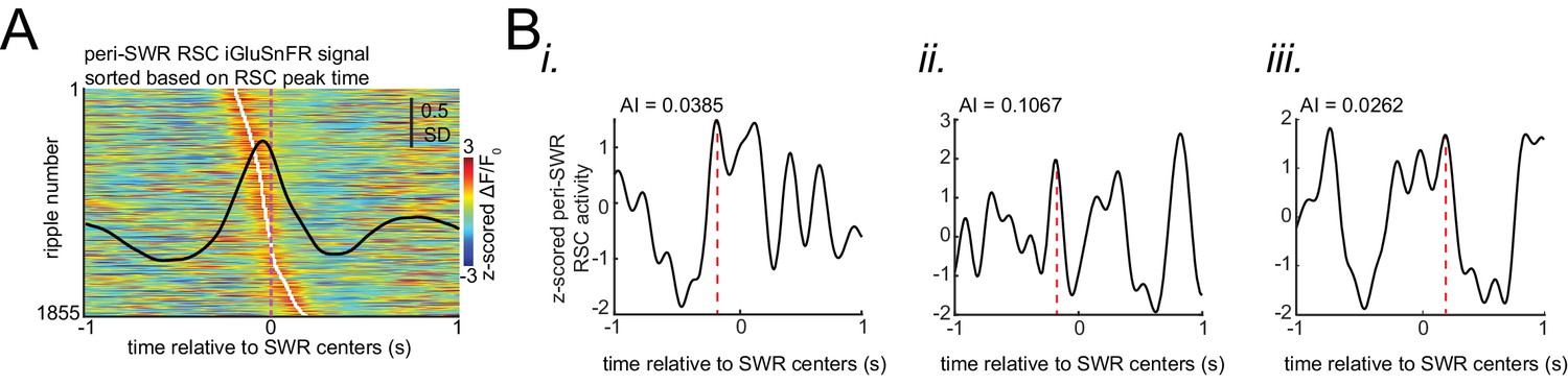
Asymmetry Index is a more robust measure of activation latency compared to peak activation timestamp.
(A) Peri-SWR RSC activity for individual SWRs sorted by peak timestamps detected in (−200 ms, 200 ms) interval. Peak timestamps were calculated for each individual peri-SWR RSC trace. Color bar represents the z-scored iGluSnFR signal. The black trace shows the mean peri-SWR RSC iGluSnFR trace. (B) (i-iii) Asymmetry index (AI), calculated for three representative traces of peri-SWR RSC activity patterns, is shown to demonstrate that the peak time may not accurately reflect the timing of activation relative to SWRs. In these examples, the peak timestamp (magenta lines) for the first two and for the third examples occur before and after the SWR time (0 s), respectively, suggesting that the corresponding SWRs have occurred in the late and early phases of RSC activation, respectively. However, the RSC AI values for these three traces do not match with this conclusion. Instead, the RSC AI values suggest that their corresponding SWRs have occurred around the middle phase of RSC activation for the first (AI = 0.0385) and third (AI = 0.0262) time traces because their corresponding AI values are close to zero, and at the early phase of RSC activation for the second (AI = 0.1067) time trace because its corresponding AI value is positive and away from zero.
Figure 5—figure supplement 2
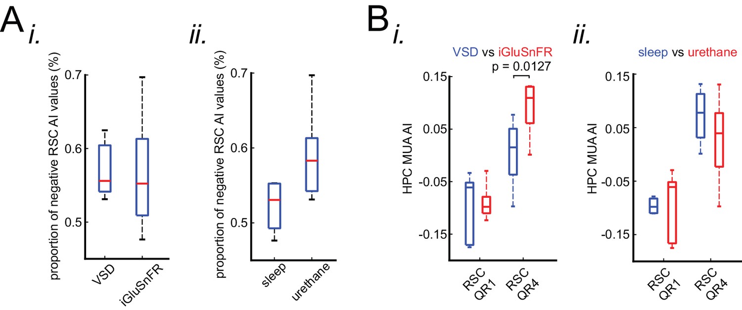
Neocortical activation latency relative to SWRs is similar under sleep/urethane anesthesia and VSD/iGluSnFR imaging conditions.
(A) There is no statistically significant difference in the proportion of negative RSC AI values in VSD versus iGluSnFR (i) nor in sleep versus urethane (ii) conditions. (B) The comparison of the distribution of medians of HPC MUA AI values across RSC QR1 and RSC QR4 in VSD versus iGluSnFR (i) and in sleep versus urethane (ii) conditions. A statistically significant difference was observed in comparing the HPC MUA AI median values for RSC QR4 in VSD versus iGluSnFR.
Figure 5—figure supplement 3
A delayed neocortical activation after SWRs in RSC QR1 was not observed.
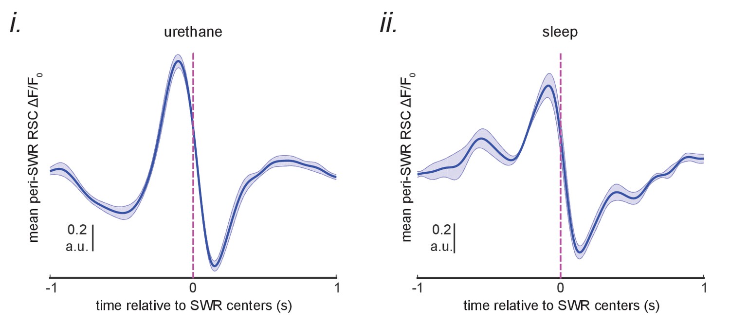
The mean of the peri-SWR RSC activity for SWRs in the RSC QR1 (blue curve shown in Figure 5Bii) were calculated for each animal and then the resultant signals were averaged across urethane-anesthetized (i) and sleeping (ii) animals separately.
Figure 6 with 2 supplements
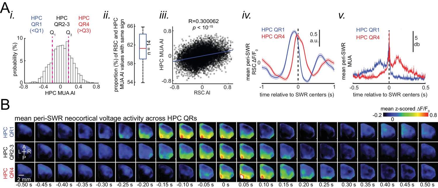
Skewness of peri-SWR hippocampal MUA informs neocortical activation latency relative to SWRs.
(A) (i) Distribution of hippocampal MUA AI values for a representative animal. Dashed lines (Q1 and Q3) indicate the first and third quartiles. The SWRs for which the associated hippocampal MUA AI values are less than Q1 and greater than Q3 are called HPC QR1 and QR4, respectively. HPC QR2-3 consists of all other SWRs. (ii) Distribution of the proportion of SWRs in each animal for which the sign of both RSC and hippocampal MUA AI values match, as an indication of how well hippocampal MUA can inform whether RSC activity precedes or follows SWRs. The horizontal red line indicates the median of all proportion values in n = 14 animals (significantly above the chance level of 50%; two-sided Wilcoxon signed rank test p=1.220703125 × 10⁻⁴). (iii) Correlation between the RSC and hippocampal MUA AI values pooled across all animals (14 animals) is low but significant (n = 11725 SWRs across all animals; two-sided t-test p<10−15). (iv) Example plots of mean peri-SWR RSC glutamate activity associated with HPC QR1 (blue) and QR4 (red). (v) Time course of exemplar mean peri-SWR HPC MUA traces associated with SWRs in HPC QR1 (blue) and Q4 (red). Notice that both HPC MUA activity (v) and RSC glutamate activity (iv) are negatively skewed (negative AI) for HPC QR1, and the converse is true for HPC QR4. (B) Mean neocortical voltage activity centered on SWR centers associated with HPC QR1, QR2-3, and QR4 in a representative animal. Note the relative temporal shift in activity across three quartile ranges. This figure has two figure supplement.
Figure 6—figure supplement 1
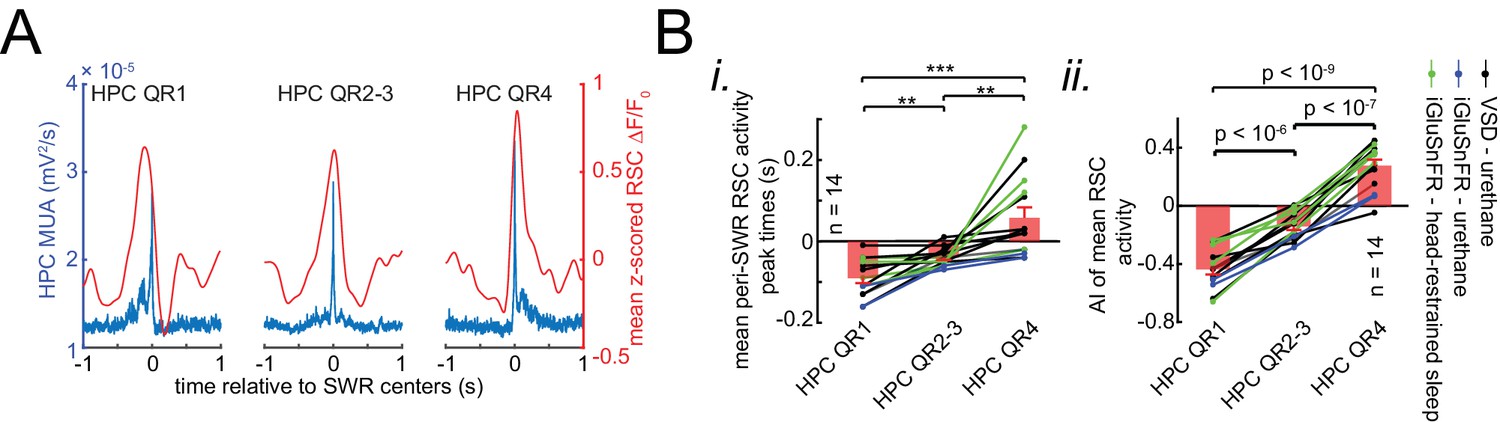
Whether retrosplenial cortex activation precedes or follows SWRs is correlated by skewness peri-SWR hippocampal MUA.
(A) Representative mean peri-SWR RSC activity (red traces) and hippocampal MUA (blue traces) calculated for hippocampal SWRs in HPC QR1, QR2-3, and QR4 defined in Figure 6A i. Notice that skewness of RSC activity and hippocampal MUA matches in each plot. (B) (i–ii) Group data (n = 14) representing the peak timestamps (i) and AI values (ii) calculated from mean peri-SWR RSC traces (red traces in panel A). Both graphs show that mean peri-SWR activation tends to precede and follow the SWRs in HPC QR1 and QR4, respectively. Bar graphs represent mean ± SEM.; **p<0.01, ***p<0.001, one-sided paired t-test.
Figure 6—figure supplement 2
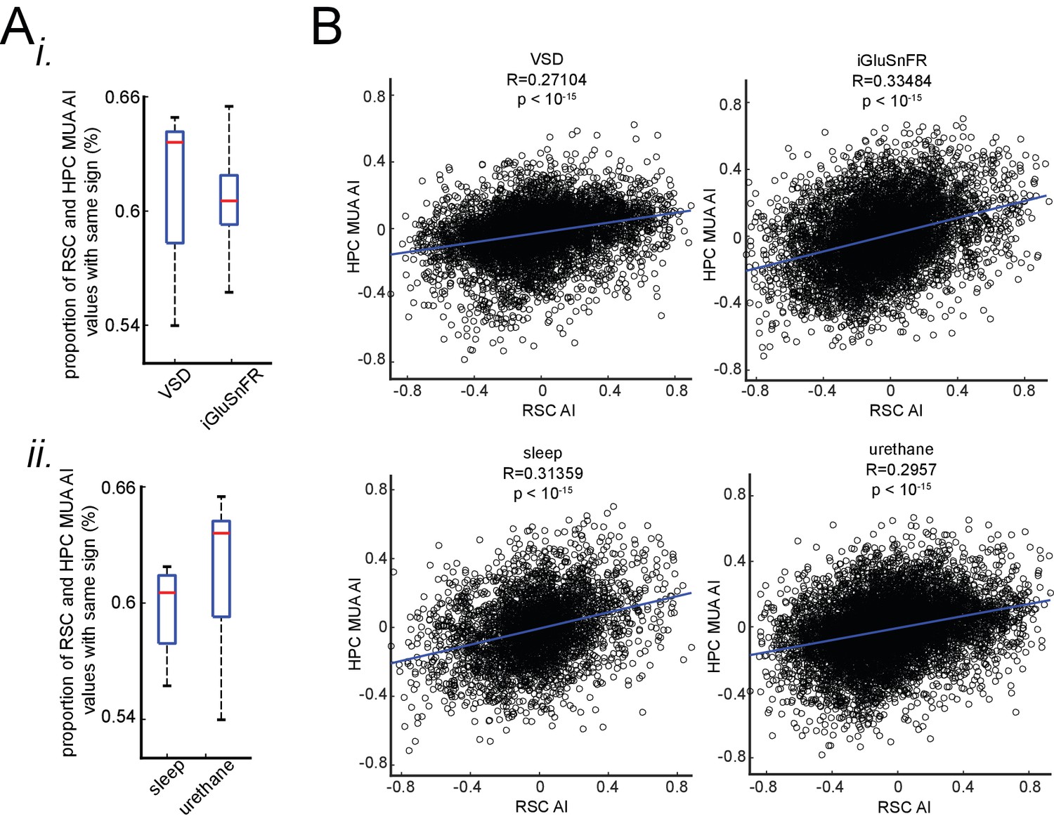
The correspondence between neocortical activation latency relative to SWRs and skewness of peri-SWR hippocampal MUA is similar under sleep/urethane anesthesia and VSD/iGluSnFR imaging conditions.
(A) There is no statistically significant difference in the proportion of RSC and HPC MUA AI values with the same sign in VSD versus iGluSnFR (i) nor sleep versus urethane (ii) conditions. (B) The correlation coefficients between RSC and HPC MUA AI values are statistically significant across all four conditions and are close to each other.
Figure 7 with 3 supplements
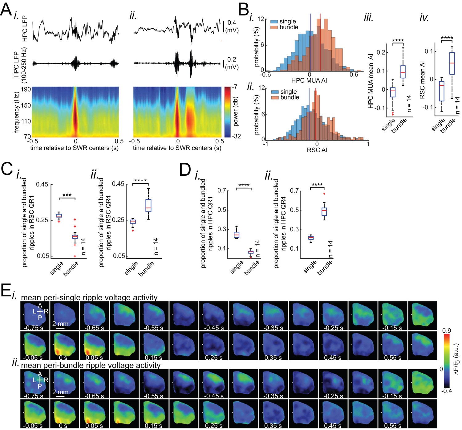
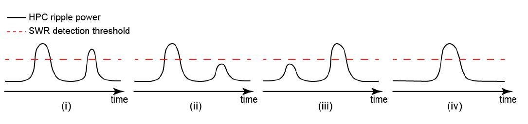
Occurrence of single/isolated ripples versus ripple bundles correlates with whether RSC activation precedes or follows hippocampus.
(A) Example raw hippocampal LFP signal (top row), ripple-band filtered signal (middle row), and mean peri-SWR spectrogram (bottom row) displaying (i) single/isolated and (ii) bundled ripples. (B) Distribution of HPC MUA (i) and RSC (ii) AI values calculated for single/isolated (blue) and bundled (red) ripples in a representative animal. The blue and red vertical lines represent the means of blue and red distributions, respectively. As expected, the red distribution is shifted to the right with respect to the blue one. (iii-iv) Comparison of HPC MUA (iii) and RSC (iv) AI mean values for single/isolated and bundled ripples (n = 14; one-sided paired Wilcoxon signed-rank test; in iii p=6.103 × 10⁻⁵; in iv p=6.103 × 10⁻⁵). The red plus signs represent the data points outside the interval (centered on median value) which includes 99.3 percent of all data points. Red horizontal lines represent the medians. (C–D) Summary data from n = 14 mice representing the proportion of single/isolated versus bundled ripples fell in RSC (C) and HPC (D) QR1 (i) and QR4 (ii). Note that there is a higher chance for single/isolated ripples to lie in RSC or HPC QR1 and higher chance for bundled ripples to fall in RSC or HPC QR4 (one-sided paired Wilcoxon signed-rank test; in C p=1.221 × 10⁻⁴; in D p=6.103 × 10⁻⁵). (E) (i–ii) Representative montages of mean neocortical voltage activity centered on single/isolated ripples (i) and the first ripple in bundled ripples (ii). Notice that neocortex stays active longer and peaks later around bundled versus single/isolated ripples. Moreover, there is strong neocortical deactivation preceding bundled ripples. This figure has two figure supplement.
-
Figure 7—source data 1
Comparing HPC MUA AI mean values across single and bundled ripples.
- https://cdn.elifesciences.org/articles/51972/elife-51972-fig7-data1-v3.mat
-
Figure 7—source data 2
Comparing RSC AI mean values across single and bundled ripples.
- https://cdn.elifesciences.org/articles/51972/elife-51972-fig7-data2-v3.mat
-
Figure 7—source data 3
Comparing the proportion of single versus bundled ripples in RSC QR1.
- https://cdn.elifesciences.org/articles/51972/elife-51972-fig7-data3-v3.mat
-
Figure 7—source data 4
Comparing the proportion of single versus bundled ripples in RSC QR4.
- https://cdn.elifesciences.org/articles/51972/elife-51972-fig7-data4-v3.mat
-
Figure 7—source data 5
Comparing the proportion of single versus bundled ripples in HPC QR1.
- https://cdn.elifesciences.org/articles/51972/elife-51972-fig7-data5-v3.mat
-
Figure 7—source data 6
Comparing the proportion of single versus bundled ripples in HPC QR4.
- https://cdn.elifesciences.org/articles/51972/elife-51972-fig7-data6-v3.mat
Figure 7—figure supplement 1

Distinct latency, strength, and duration of neocortical modulation around single/isolated versus bundled ripples.
(A) (i–ii) Peri-SWR RSC activity for individual single/isolated (i) and bundled (ii) SWRs sorted by RSC asymmetry index. Asymmetry indices were calculated for each individual peri-SWR RSC trace. Color bar represents the z-scored iGluSnFR signal. The black trace shows the mean peri-SWR RSC iGluSnFR trace. The peri-SWR RSC traces in bundled ripples are wider and cover longer post-ripple time durations, demonstrating the reason why the distribution of RSC Asymmetry Index (AI) values for bundled ripples tends to have larger median values compared to single/isolated ripples. (B) Schematic of a cranial window for optical imaging of neocortical voltage or glutamate activity. The voltage or glutamate activity was recorded from the dorsal surface of the right neocortical hemisphere, containing the specified regions. The abbreviations denote the following cortices AC/M2: anterior cingulate/secondary Motor, RS: retrosplenial, M1: primary motor, HLS1: hindlimb primary somatosensory, PtA: posterior parietal, V2M: secondary medial visual, FLS1: forelimb primary somatosensory, TrS1: trunk primary somatosensory, ShNcS1: shoulder/neck primary somatosensory, V1: primary visual, ULpS1: lip primary somatosensory, BCS1: primary barrel, V2L: secondary lateral visual, S2: secondary somatosensory, A1: primary auditory. (C–D) Neocortical activation (C) and deactivation (D) peak timestamps (i), activation amplitudes (ii), and durations (iii) across neocortical regions around single/isolated versus bundled ripples. Such deactivations always precede SWRs. Notice that the neocortical activation and deactivation peak timestamp is significantly larger around bundled compared to isolated ripples in all (almost all for deactivation) neocortical regions. Moreover, the significant difference in activation and deactivation amplitudes around isolated versus bundled ripples is observed in all neocortical subnetworks (except the medial one for activation). The duration of neocortical activation is longer in all neocortical subnetworks around bundled compared to single/isolated ripples while that of deactivation is longer only in the medial subnetwork (*p<0.05, **p<0.01, ***p<0.001, n.s. p>0.05, paired t-test; n = 13–14 mice). All bar graphs represent mean ± SEM.
Figure 7—figure supplement 2
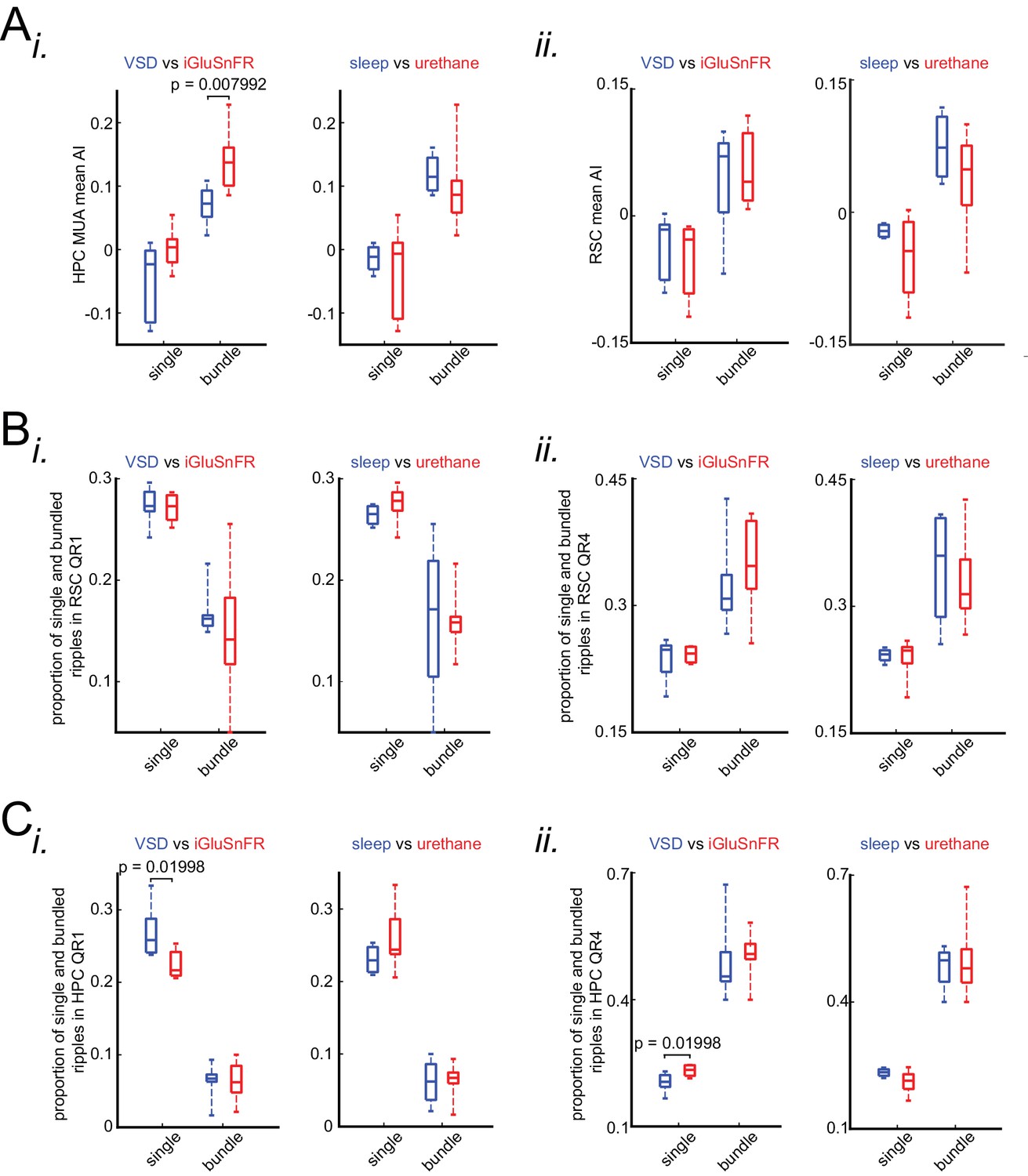
The correlation between occurrence of single/isolated versus bundled ripples and latency of peri-SWR RSC activation is similar under sleep/urethane anesthesia and VSD/iGluSnFR imaging conditions.
(A) Comparison of HPC MUA (i) and RSC (ii) mean AI values in VSD versus iGluSnFR and in sleep versus urethane conditions across single and bundled ripples. The only statistically significant difference is from comparing HPC MUA mean AI values of bundled ripples in VSD versus iGluSnFR conditions. (B) Comparison of proportion of single and bundled ripples in RSC QR1 (i) and RSC QR4 (ii) in VSD versus iGluSnFR and sleep versus urethane conditions. There is no statistically significant in all eight comparisons here. (C) The same as B except for HPC QR1 (i) and HPC QR4 (ii). There are two statistically significant differences out of eight comparisons here. P-values for these significant differences are shown in the diagrams.
Figure 7—video 1
Mean peri-single-SWR versus peri-bundled-SWR voltage activity under urethane anesthesia.
Example of mean peri-SWR voltage activity around single/isolated versus bundled SWRs. The spectrograms represent the mean frequency content of peri-SWR hippocampal LFP around single/isolated versus bundled SWRs.
Author response image 1
Author response image 2
Additional files
Download links
A two-part list of links to download the article, or parts of the article, in various formats.
Downloads (link to download the article as PDF)
Open citations (links to open the citations from this article in various online reference manager services)
Cite this article (links to download the citations from this article in formats compatible with various reference manager tools)
Spatiotemporal patterns of neocortical activity around hippocampal sharp-wave ripples
eLife 9:e51972.
https://doi.org/10.7554/eLife.51972


