Elements of a stochastic 3D prediction engine in larval zebrafish prey capture
- Harvard University, United States
- Massachusetts Institute of Technology, United States
Figures
Figure 1 with 2 supplements
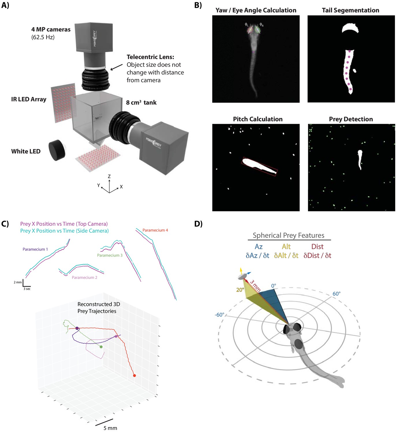
A novel 3D experimental paradigm for mapping prey trajectories to fish movement choices.
(A) 3D rendering of rig design and features. (B) Computer vision algorithms extract the continuous eye angle, yaw, pitch, and tail angle of the zebrafish. In every frame, prey are detected using a contour finding algorithm. (C) Prey contours from the two cameras are matched in time using a correlation and 3D distance-based algorithm, allowing 3D reconstruction of prey trajectories. (D) Prey features are mapped to a spherical coordinate system originating at the fish’s mouth. Altitude is positive above the fish, negative below. Azimuth is positive right of the fish, negative left. Distance is the magnitude of the vector pointing from the fish’s mouth to the prey.
Figure 1—figure supplement 1
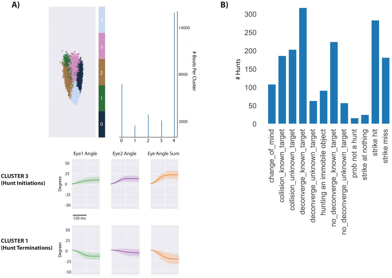
Identificaiton of hunt sequences.
(A) Spectral clustering (scikit-learn) was used to cluster the continuous eye angle over each bout for both eyes. The initiation of hunt sequences was identified using Cluster three and deconvergence of the eyes was demarked by Cluster 1. (B) Hunt sequence types in the dataset. The user’s only role is to denote the last bout of the hunt sequence, characterize the sequence as a strike hit, strike miss, or abort, and note the chosen prey ID assigned by our automated prey reconstruction algorithm. The program then outputs the descriptors in B per hunt. ‘Collisions’ imply that the fish head has collided with the wall during the hunt (detected using fish COM and edge coordinates), preventing analysis of whether the fish would have struck or aborted. Collisions with unknown target are likely hunting of a paramecium reflection. Deconvergence, known target and unknown target, is the standard abort described previously (Johnson et al., 2019; Henriques et al., 2019), with ‘unknown targets’ being too ambiguous for the user to make a call on pursued prey ID. No deconvergence, known target are hunts where fish had initiated to and pursued a particular prey item, but clearly stopped pursuit on a particular bout not assigned to Cluster 1. ‘Probably not a hunt’ was a rare case where the fish converged, swam through the tank without choosing a prey, and did not deconverge within eight bouts. ‘Strike at Nothing’ was another rare case where the fish converged and struck without a prey item present. The fish did spend some time striking at immobile objects that were almost invariably residue stuck to the top of the tank. During strike hits, fish choose a prey and consume it, with strike misses typically a deflection of the prey off the fish’s mouth at hunt termination. The main manuscript is built off of strike hits and misses (which combined into a ‘strikes at known prey’ category would be the most common outcome), while Supplementary Figure 3’s abort algorithm is built from known target, deconverge and no-deconverge hunts. Collisions are simply an outcome of having a relatively small tank for parfocal imaging compared to the fish’s real environment; hunts resulting in collisions were not analyzed except for the initial choice.
Figure 1—figure supplement 2
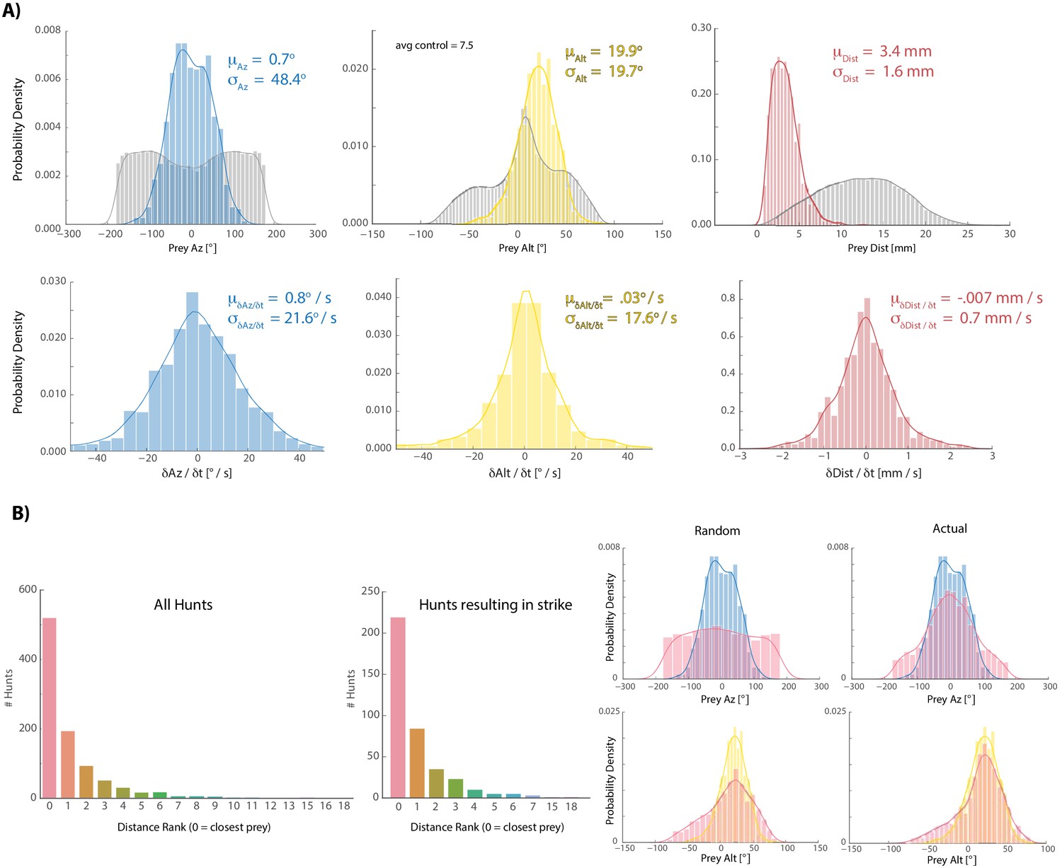
Fish tend to choose the closest available prey when initiating hunt sequences.
(A) Colors are histograms of coordinates for prey chosen at hunt initiation, gray are all prey records [chosen + ignored. Note: XY records passing a threshold length and velocity that remain unpaired after prey reconstruction are assigned the Z-coordinate of the tank ceiling because live paramecia show anti-gravitaxis (Roberts 2010); we always noted that a subset of prey gather at the ceiling and never noticed coagulation of prey on the ground unless dead; results are very similar to those shown if ceiling assigned prey are not counted]. (B) Histograms showing the distribution of spherical velocities for chosen prey do not reveal a bias in magnitude or direction. (C) Count plots of distance rank for selected prey (0 = closest). (D) We virtually displaced fish coordinates at hunt initiation bouts into randomly recorded paramecium environments and asked whether the closest prey item in that environment shared azimuth and altitude features with prey that fish actually chose. Histograms of the closest prey in random prey environments and prey environments in which initiation actually occurred are plotted in red (for random condition, fish orientation and position at hunt initiation is projected into a different time during the experiment; left panel). Blue (az) and yellow (alt) histograms are chosen prey histograms from (A) for comparison. The closest prey item in a random environment does not show the same distribution as selected prey in (A), indicating that the closest prey does not necessarily have to share the altitude and azimuth features of chosen prey. This suggests that somewhat specific prey features are preferred for entry into the hunting state, although transition probabilities governing hunting mode entry are also at play (Johnson et al., 2019; Mearns et al., 2019).
-
Figure 1—figure supplement 2—source data 1
Source data describing prey at hunt initiations.
- https://cdn.elifesciences.org/articles/51975/elife-51975-fig1-figsupp2-data1-v2.zip
Figure 2 with 1 supplement
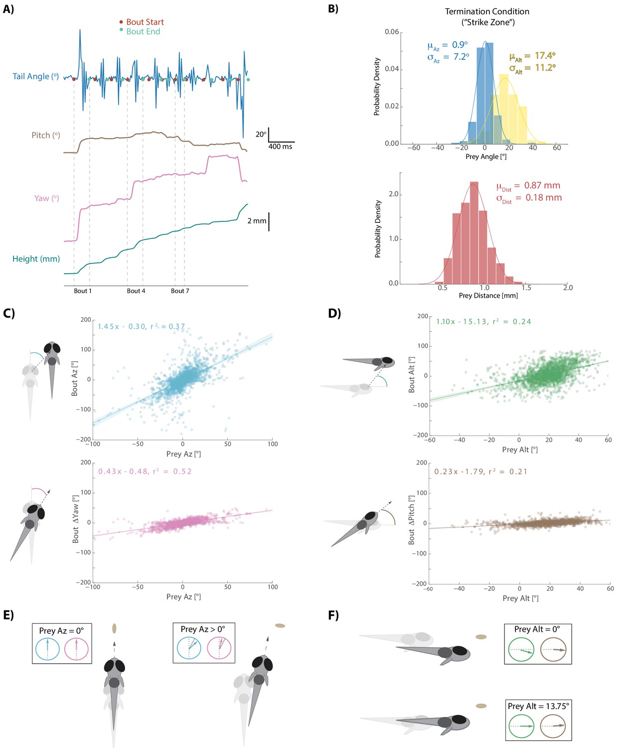
Fish execute 3D movements based on the position of their prey.
(A) During hunt sequences, fish swim in bouts that can be detected using tail variance. Bouts can change the yaw, pitch, and position of the fish, while time between bouts is marked by quiescence. (B) Histograms showing the distributions of spherical prey positions when fish successfully ate a paramecium during a strike. (C, D) Regression fits between prey position and bout variables executed by the fish. (E, F) Features of sensorimotor transformations based on prey position: fish swim forward if prey are directly in front. Otherwise, if prey are on right, fish displace and rotate right; and vice versa. Fish displace downward if prey are at 0° altitude, but displace with no altitude change if prey are at 13.75°. In all schematics (C–F), positions and orientations at the beginning of the bout are represented by transparent fish, and by opaque fish at the end of the bout.
-
Figure 2—source data 1
Source data for all bouts conducted in dataset.
- https://cdn.elifesciences.org/articles/51975/elife-51975-fig2-data1-v2.zip
Figure 2—figure supplement 1

Prey capture algorithm during aborted hunt sequences.
(A) Regression fits between prey position and bout variables during hunt sequences ending in an abort. Gray points and lines represent the last three pursuit bouts before the quit bout occurs, colors are all bouts between initiation and the last 3. The algorithm strongly resembles Figure 2 transformations at the beginning of hunt sequences that will eventually end in aborts, but goes awry in the last three bouts before quitting. (B) Pursuit bouts during abort sequences show modulation by velocity at inflection points similar to Figure 3—figure supplement 1B. (C) Orange model is the same as Figure 4 (Orange Model 2), which issues bouts based on multiple regression to prey position variables only. Green model is same as Figure 4 (Green Model 3), which issues bouts based on multiple regression to prey position and velocity variables. However, both are fit using pursuit bouts during aborted sequences (outside of the last three bouts before quitting) instead of strike sequences (i.e. Figure 4). As with models fit on strike sequences, multiple regression using prey position and velocity outperforms position only regression due to proportional velocity modulation. Both models are fed the exact same prey trajectories as models in Figure 4. Fitting on pursuit bouts during aborted sequences thus shows similar performance levels to models fit on strike sequences.
Figure 3 with 1 supplement
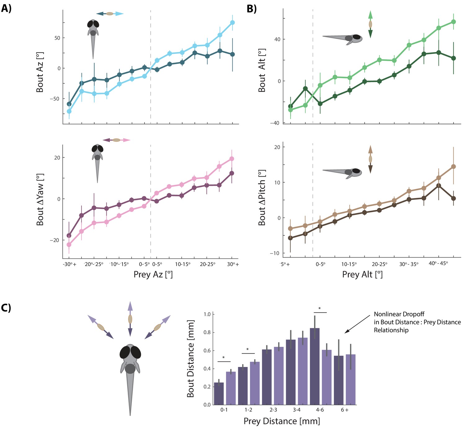
Prey velocity biases all aspects of fish's bout choices.
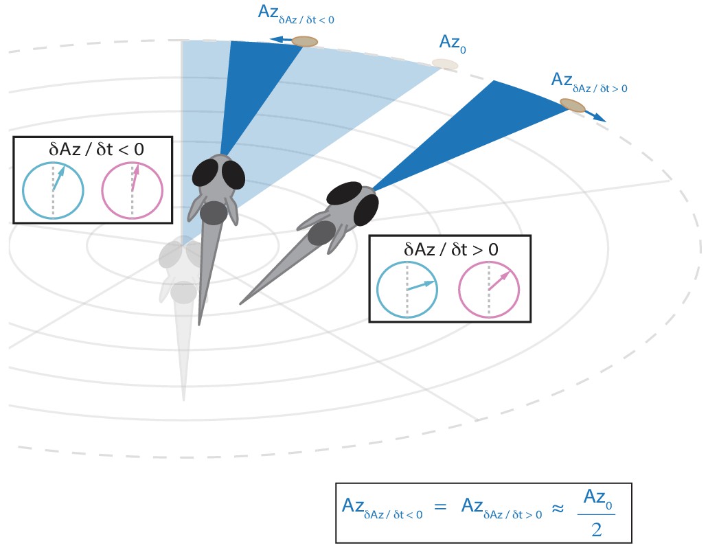
(A, B) Light colors depict each bout variable if prey are moving away from the fish while dark colors indicate that prey are moving toward the fish in the same 5° window of space. A pattern emerges of dampening movements when prey velocity is towards the fish, and amplifying movements when prey velocity is away from the fish. Point locations are means with error bars representing 95% CIs. Multiple regression fitting of bout variables to prey position and velocity in all planes confirm and quantify the dampening and amplification (azimuth velocity moving left to right of the fish is positive, altitude velocity upward is positive). Bout Az is biased by .251 * Prey δAz / δt (.219 - .283 95% CI), Bout ΔYaw by .054 * Prey δAz / δt (.046-.061 95% CI), Bout Alt by .300 * Prey δAlt / δt (.268 - .331 95% CI), and Bout ΔPitch by .031 * Prey δAlt / δt (.024 - .039 95% CI). Dividing these coefficients by the average bout length (0.176 s) yields the projected positional coefficients described in the text. (C) Bout Distance is linearly proportional to Prey Distance but only within 4 mm of the fish, with breakdown in relationship above 6 mm. Likewise, dampening of Bout Distance when Prey δDist / δt < 0 (prey approaching radially), and amplifying when Prey δDist / δt > 0 (prey moving afar), occurs in two windows: 0–1 mm, and 1–2 mm from the fish. Overall, multiple regression finds: Bout Distance = 0.105 * Prey Dist + .053 * Prey δDist / δt (95% CIs = 0.094-.116, .034-.071), which reflects the fact that ~70% of pursuit bouts occur when prey are within 2 mm. (*: p<0.05/6, Bonferroni corrected two-tailed t-tests. p-values: 0–1 mm = 2.7 * 10−6, 1–2 mm: 0.0016, 2–3 mm: 0.38, 3–4 mm: 0.73, 4–6 mm: .00046, 6+: 0.92).
Figure 3—figure supplement 1
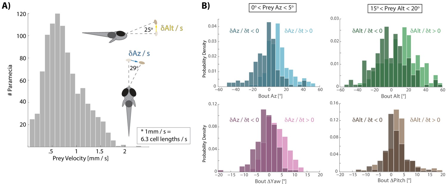
Distribution of prey velocity and example prey velocity-based biasing of bout features.
(A) Distribution of 3D velocities of prey hunted by fish in our study. Mean azimuth and altitude velocities (absolute value) are shown in reference to the fish, averaged over 80 ms before pursuit bout initiation, which is the time interval of all velocity calculations implemented here. (B) Example histograms for two 5° windows of prey space, as shown in Figure 3A,B. Again, light colors indicate that prey are moving away from the fish and dark moving toward. If prey are 0–5° to the right of the fish, but swimming toward the fish in azimuth, the fish will actually turn and displace left, predicting that the prey will cross its midline. If swimming away, fish turn and displace to the right. In a window 15–20° above the fish in altitude, the fish will actually ‘wait’ for prey with downward velocity (i.e. Bout Alt ~0°), anticipating that the prey will arrive in the strike zone. Otherwise if prey are moving upwards, fish displace and rotate upwards.
Figure 4

Virtual prey capture simulation reveals necessity of velocity perception.
(A) A virtual prey capture environment mimicking the prey capture tank was generated to test three different types of models, and six models overall, described in the schematic. Models control a virtual fish consisting of a 3D position (red dot) and a 3D unit vector pointing in the direction of the fish’s heading. Virtual fish are started at the exact position and rotation where fish initiated hunts in the dataset. Prey trajectories are launched that reconstruct the real paramecium movements that occurred during hunts. The virtual fish moves in bouts timed to real life bouts, and if the prey enters the strike zone (defined by the distributions in Figure 2B, Materials and methods), the hunt is terminated. (B) Barplots (total #) and box plots (median and quartiles) showing performance of all six models in success (# Strikes), energy use per hunt sequence, and how many bouts each model performed during the hunt (a metric of hunt speed). (C) KDE plots showing the distribution of Post-Bout Prey Az and Post-Bout Prey Alt distributions for each model during virtual hunts. Dotted lines demark the strike zone mean.
Figure 5 with 3 supplements

A cannonical 'halving' strategy emerges.
(A) Regression plots showing relationships between pre-bout prey coordinates and post-bout prey coordinates. Dark colors, prey are moving toward the fish. Light colors, prey are moving away from the fish. 95% CI on azimuth transforms’ y-intercept includes 0°. Top right panel fit on all distances < 6 mm (see Figure 3C). (B) Schematic showing recursive halving of the angle of attack during pursuit. (C) Regression slopes are constant across the hunt sequence; color coded to 5A. (D) Pseudocode describing the recursive prey capture algorithm that transforms according to 5A until it arrives at the strike zone. The combined (both velocity directions) distance transform is .84 * Pre-Bout Prey Dist -. 0125 mm = Post Bout Prey Dist. The azimuth transform is .53 * Pre-Bout Prey Az = Post Bout Prey Az. The altitude transformation is .54 * Pre-Bout Prey Alt + 8.34° = Post Bout Prey Alt. Implementing these equations recursively will terminate the algorithm at 18.1° Prey Alt (since .54 * 18.1° + 8.34° = 18.1°) and 0° Prey Az (.53 * 0° = 0°), which aligns precisely with the strike zone described in Figure 2B. See Appendix for full pseudocode of all sub-functions.
Figure 5—figure supplement 1
Schematic showing that the fish will reduce the post-bout angle of attack to the same value regardless of whether prey is moving towards or away from the fish (see Figure 5A).
Figure 5—figure supplement 2

Regression fits between Pre-Bout and Post-Bout Prey Alt differ depending on whether prey altitude is positive or negative before the bout.
Most bouts in the dataset (>92%) occur when prey are above the fish. This change when prey cross 0° Alt is accounted for in all algorithms (see Appendix).
Figure 5—figure supplement 3

Transformation by the initiation bout of Pre-Bout to Post-Bout Prey Az and Alt.
The initiation bout is a large angle turn that divides azimuth more than a pursuit bout; altitude is also significantly more reduced by the initiation bout. All regression models in simulations therefore use an independent regression fit to initiation bouts to start every simulated hunt.
Figure 6 with 1 supplement
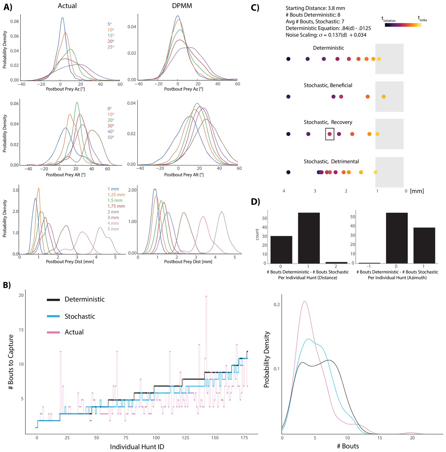
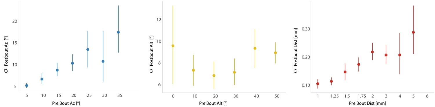
Graded stochasticity in sensorimotor transformations improves hunting performance.
(A) KDE plots of post-bout variable distributions for pre-bout input coordinates described in the legend, color-coded to the KDEs (i.e. the blue KDE in Az is the distribution of all Post-Bout Prey Az given that Pre-Bout Prey Az is 5°). Real data is binned in 5° windows for angles and. 25 mm bins for distance. DPMM-generated post-bout variables are directly simulated from the model 5000 times, conditioned on the pre-bout value in the legend. (B) The median performance of the DPMMs embedded in a recursive loop (stochastic recursion algorithm; run 200 times per initial prey position) typically ties or outperforms the deterministic recursion model, which transforms with the same pre-bout to post-bout slopes as the DPMMs. Pink line is the performance of the real fish. Right panel: KDE plot of data from 6A, showing that the stochastic algorithm approaches the speed of the real fish. (C, D) A Graded Variance Algorithm where proportional noise is injected into each choice (equations below) is applied 500 times per initial distance (0.1 mm to 10 mm, .1 mm steps) or azimuth (10° to 200° in steps of 2°). Termination condition is a window from. 1 mm to 1 mm for distance, −10° to 10° for azimuth (see Appendix for full algorithm). Deterministic recursion algorithm (Figure 5D) is also run on each initial azimuth and distance with .53 * az for azimuth and .84 * dist - .0125 mm as the fixed transforms. Graded Variance uses these exact transforms as the mean while injecting graded noise: σd = 0.137 * dist + 0.034 mm; σaz = .36 * az + 7.62°, which were fit using linear regression on samples generated by our Bayesian model (6B). (C) shows examples of Graded Variance performance (‘stochastic’) vs. deterministic performance for an example start distance of 3.8 mm. (D) is a barplot comparing the deterministic performance for each input distance and azimuth to the median Graded Variance (‘stochastic’) performance where we directly injected noise. Average performance using noise injection typically ties or defeats deterministic choices by one bout.
-
Figure 6—source data 1
Generators for BayesDB simulations.
- https://cdn.elifesciences.org/articles/51975/elife-51975-fig6-data1-v2.zip
Figure 6—figure supplement 1
Standard deviation is plotted for each individual fish per five degree bin of prey space, indicating that graded stochasticity is not simply observed in the pooled bout population, but at the level of single fish.
Videos
Video 1
In each instance, a hunt is shown from the top and side cameras simultaneously, followed by a virtual reality reconstruction of the fish’s point of view during the hunt.
The virtual reality reconstruction, built in Panda3D, is generated from 3D prey coordinates and unit vectors derived from the 3D position, pitch, and yaw of the fish.
Video 2
Virtual prey capture simulation environment.
Each model from Figure 4 begins at the same position and orientation and is given the task of hunting the same paramecium trajectory. In this representative hunt sequence, every model except the Random Choice and Multiple Regression (Position Only) models consume the prey (indicated by red STRIKE flash). As is typical in the simulations, the Ideal Choice (Position) model lags the Ideal Choice (Velocity) model by one bout.
Tables
Key resources table
| Reagent type (species) or resource | Designation | Source or reference | Identifiers | Additional information |
|---|---|---|---|---|
| Software, algorithm | BayesDB | arxiv | arxiv:1512.05006 | http://probcomp.csail.mit.edu/software/bayesdb/ |
| Strain, strain background (Danio rerio) | WIK | ZFIN | ZFIN_ZDB-GENO-010531–2 |
Additional files
Download links
A two-part list of links to download the article, or parts of the article, in various formats.
Downloads (link to download the article as PDF)
Open citations (links to open the citations from this article in various online reference manager services)
Cite this article (links to download the citations from this article in formats compatible with various reference manager tools)
Elements of a stochastic 3D prediction engine in larval zebrafish prey capture
eLife 8:e51975.
https://doi.org/10.7554/eLife.51975


