Tuning movement for sensing in an uncertain world
- Center for Robotics and Biosystems, Northwestern University, United States
- Department of Biomedical Engineering, Northwestern University, United States
- Department of Mechanical Engineering, Northwestern University, United States
- Department of Neurobiology, Northwestern University, United States
Figures
Figure 1 with 1 supplement
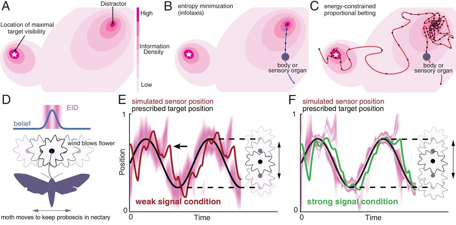
Illustration of a 2-D expected information density, information maximization and energy-constrained proportional betting.
(A) The heat map represents the expected information density. Because the peak expected information is typically not at the same location as the object, we illustrate the target peak as the point of maximum target visibility. (B) Trajectories generated by information maximization (entropy minimization) locally maximizes the expected information density (EID) at every step, which here commands a path straight to the nearby distractor. In contrast, energy-constrained proportional betting (C) samples the EID proportionate to its density and is balanced by the cost of movement. The natural trade-off between exploration and exploitation that emerges leads to localization of the target and rejection of the distractor (adapted from Figure 3 of Miller et al., 2016). Black dots along the trajectory indicate samples at fixed time intervals (longer distances between dots indicate higher speed). (D–F) An illustration of an animal tracking an object constrained to movement in a line, in this case a hypothetical moth using visual signals to track a flower it is feeding from while the flower sways in a breeze in a manner approximated by a 1-D sinusoid—a natural behavior (Sponberg et al., 2015). We simulate the tracking of the flower using the ergodic information harvesting algorithm, our implementation of energy-constrained proportional betting. (D) In the top panel, we show an idealization of the moth’s belief about the flower’s location when the flower reaches the center point (blue line Gaussian distribution above the moth). Higher values in the direction represents higher confidence of the target at the given location. The corresponding EID is overlaid in magenta; a darker color indicates higher expected information should the animal take a new sensory measurement in the corresponding location. Note the bimodal structure of this highly idealized EID, with identical maximal information peaks on both sides of the Gaussian belief peak. Intuitively, the expected information is higher along the high slope region of the belief because in this region, small changes in location (x axis direction in the upper inset) is expected to cause large changes in the received sensory signal and hence carry more information about position. (E) Simulation of the moth’s position (red curve) while tracking a swaying flower (black curve) in dim light. The corresponding EID is overlaid in magenta. Energy-constrained proportional betting results in persistent activation of movement when the EID is relatively diffuse due to lack of information. Note the presence of a fictive distractor (marked by the black arrow) in the EID due to higher uncertainty in the sensory input as a result of the weaker signal. As seen by the digression at the arrow, ergodic information harvesting (EIH) responded to the distractor by making a detour away from the actual target position to gamble on the chance of acquiring more information but does not get trapped by the distractor because of the proportional betting strategy in combination with the transient nature of fictive distractors. (F) Same as (E), but under strong signal conditions. Now the energy-constrained proportional betting trajectory samples both peaks of the bimodal EID with excursions away from these peaks, similar to measured moth behavior (Stöckl et al., 2017, see Figure 1—figure supplement 1 ‘Moth’). Note that even though trajectory segments are planned at 14 fixed-time intervals T (Materials and methods) over the shown duration based on the EID at the start of those intervals, the EID is here plotted continuously for visualization purposes only.
Figure 1—figure supplement 1

Whole-body or sensory organ small-amplitude motions are ubiquitous as animals track targets.
Here we show siphon casting behavior in the marine snail (body, Ferner and Weissburg, 2005), cross-current swimming in the Chambered nautilus (body, Basil et al., 2000), whole-body oscillations in electric fish (body, Stamper et al., 2012), zigzagging motions in the rat (nose, Khan et al., 2012), back and forth searching in the mole (nose, Catania, 2013), fixational eye movements in humans (eye, Rucci and Victor, 2015), the zigzagging walk of the cockroach (head, Willis and Avondet, 2005), and flower tracking motions in the moth (head, Stöckl et al., 2017). These sensing-related movements occur with striking consistency across animals using different sensory modalities and within different physical environments. We propose these movements arise as a form of gambling on information through motion, and show evidence in support of this claim from the four species highlighted (electric fish, mole, cockroach, and moth). Photo credit: Schulz, 2014 Marine snail image courtesy of Katja Schulz, under a CC BY 2.0 generic license; Kirk, 2008 Eigenmannia image courtesy of Will Kirk, composite image composed and edited by Eric Fortune and Eatai Roth, under a CC BY 2.5 generic license.
© Berger, 2007. Chambered nautilus image courtesy of Lee Berger. Published under a CC BY SA 3.0 unported license.
© Poirrier, 2007. Rat image courtesy of Jean-Etienne Minh-Duy Poirrier. Published under a CC BY SA 2.0 license.
© Catania, 2008. Mole image courtesy of Kenneth Catania. Published under a CC BY SA 3.0 unported license.
© Wikimedia Commons, 2013. Human image courtesy of Wikimedia Commons. Published under a CC BY SA 3.0 unported license.
© Wikimedia Commons, 2013. Cockroach image courtesy of Wikimedia Commons. Published under a CC BY SA 3.0 unported license.
© Wikimedia Commons, 2006. Moth image courtesy of Wikimedia Commons. Published under a CC BY SA 3.0 unported license.
Figure 2 with 3 supplements
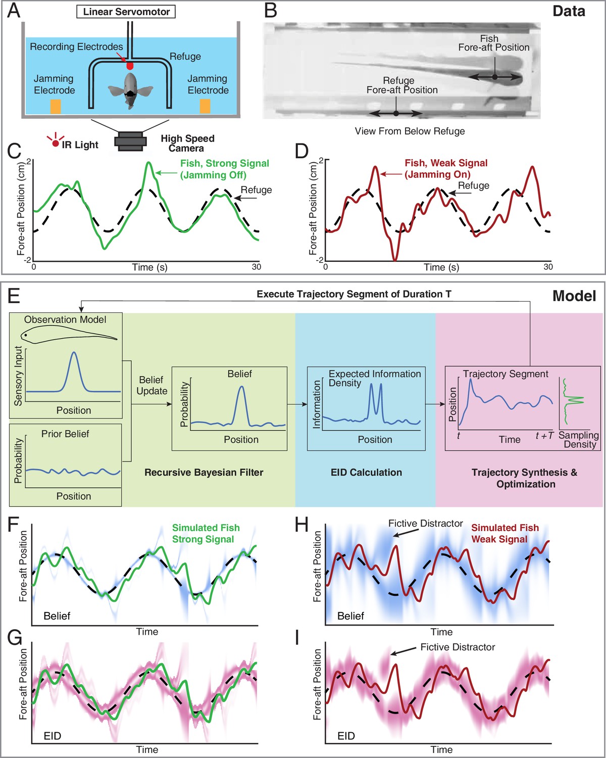
Longitudinal refuge tracking behavior in weakly electric fish and core components of EIH.
(A) Head-on view of experimental apparatus. A computer-controlled linear servo moves the refuge forward and backward along the longitudinal axis of the fish. Jamming electrodes are mounted to the side of the tank and recording electrodes are mounted to the ends of the refuge to generate and monitor the level of electrosensory noise (Materials and methods). (B) An example frame of the captured video. (C–D) Fish tracking the refuge in the strong signal condition (no jamming applied), and in the weak signal condition (with jamming). Note that departures from the refuge position occur more often and with larger amplitude in the weak signal condition (Stamper et al., 2012). (E) Core components of the EIH algorithm, shown by colored blocks: a recursive Bayesian filter (green block), an EID calculation (blue block), and synthesis and optimization of a trajectory segment (pink block). The process starts with the simulated fish receiving new sensory input via its position and the observation model. Through the recursive Bayesian filter process, the simulated fish updates its prior belief about the refuge’s true location (the belief is initially uniform since the location is unknown) and captures that increase in information in a posterior belief. It then computes the EID based on the posterior belief, explaining why the EID is bimodal when the variance in the estimate is low for the Gaussian observation model: Figure 1D and G. A trajectory segment is then computed that balances proportional betting on the EID (ergodicity) with the cost of movement. The resulting trajectory samples locations proportionate to the EID, as shown by the Sampling Density plot. After these three stages, the simulated fish executes the trajectory segment and returns to begin the process again. (F, G) Simulated fish behavior in the strong signal condition. The blue heatmap shows belief (top) of where the target is, where darker colors represent locations with higher probability, and expected information density (bottom) is represented by the magenta heatmap where darker colors represent higher expected information. (H, I) As in F, G, but for the weak signal condition. As in the experimental observations, the departures from the refuge’s path are larger and more frequent in the weak signal condition. Note the presence of various color bands representing fictive distractors.
Figure 2—figure supplement 1
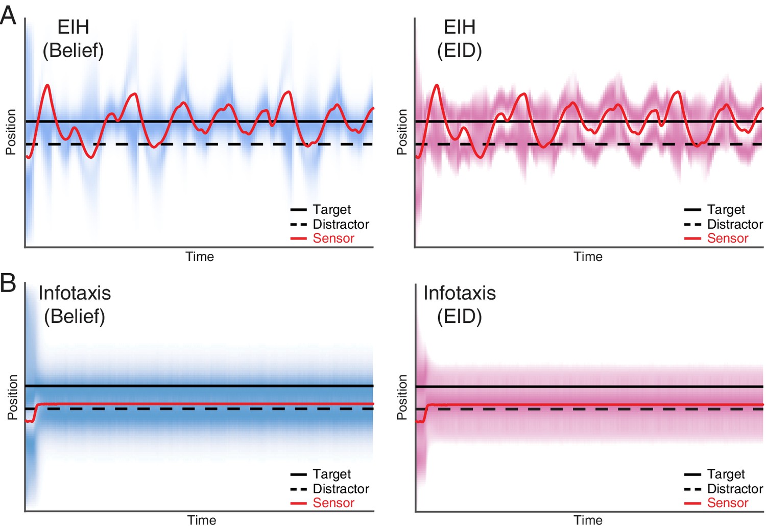
Single target tracking simulation with EIH and infotaxis in the presence of a simulated physical distractor.
In this simulation, a single target and a physical distractor coexist in the workspace. The simulated physical distractor has a different observation model that leads to a different measurement profile when compared to the desired target. To help visualize the outcome, the belief (left panel) and EID (right panel) distribution over time are rendered with blue and magenta color overlay, respectively. In both cases, we use identical SNR levels corresponding to a weak signal condition (30 dB, see Table 2). (A) EIH is able to find the desired target (the continuous peak along the desired target location in the left panel) and rejects the distractor (no continuous peak along the distractor location in the left panel). (B) Infotaxis gets trapped at one of the information maximizing peaks, as seen in the right panel. Although it does find the desired target, it fails to reject the distractor, as seen in the continuous peak near the distractor in the left panel.
Figure 2—figure supplement 2
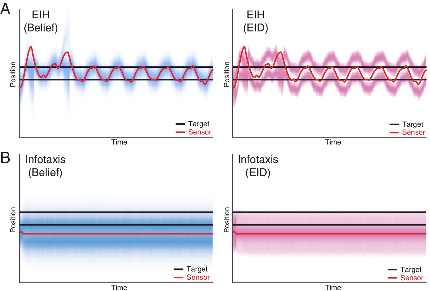
Dual target tracking simulation with EIH and infotaxis.
In this simulation, two identical targets (with the same observation model) are present in the workspace, indicated by the two blue lines. To help visualize the outcome, the belief (left panel) and EID (right panel) distribution over time are rendered with blue and magenta color overlay, respectively. In both cases, we use identical SNR levels corresponding to a weak signal condition (30 dB, see Table 2). (A) EIH tracks both targets with an oscillatory motion. In addition, belief peaks corresponding to the top and bottom targets are clearly visible in the left panel. (B) Infotaxis gets trapped at one of the information maximizing peaks, as seen in the right panel. This leads to cessation of movement and failure to detect the other target on the top (left panel).
Figure 2—figure supplement 3
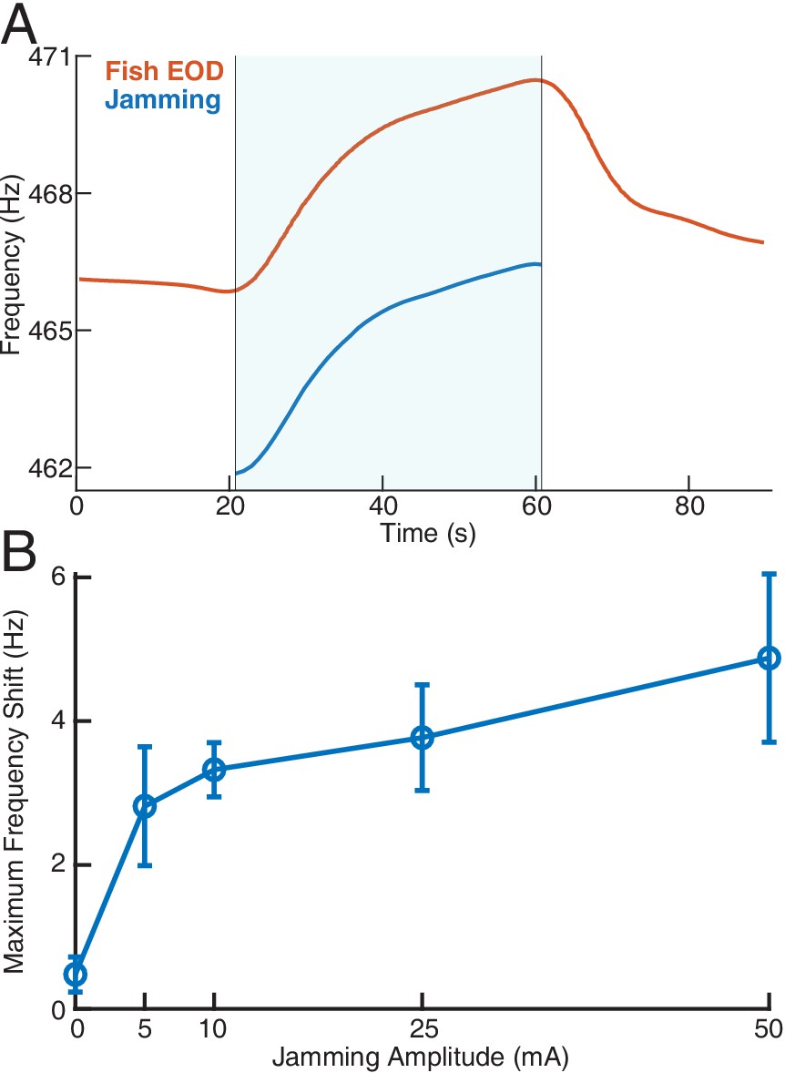
Effect of jamming and how it varies with jamming intensity.
(A) A representative trial of how a fish’s electric organ discharge (EOD) frequency shifts up continuously as the jamming signal is being applied. The area shaded with light blue indicates when jamming is turned on and lasts 40 s. The jamming signal frequency (current amplitude = 25 mA) is set to be 5 Hz below the fish’s EOD frequency. The fish’s EOD frequency gradually declines back to its normal value after jamming is turned off after around 60 s. (B) Maximum frequency shift during the fixed 40 s jamming window as a function of jamming current amplitude. The average maximum frequency shift for every jamming amplitude across a total of 26 trials is marked by the circle ( for 0 mA, for 5 mA, for 10 mA, for 25 mA, for 50 mA), with ±1 standard deviation illustrated by the error bar. The amount of jamming applied has a clear positive correlation with the EOD frequency shift.
Figure 3

Fish behavior versus EIH predictions.
(A) Relative exploration values (defined in text) for the fish and EIH trajectories under strong and weak signal conditions. Each dot represents a behavioral trial or simulation. EIH (bottom row) shows good agreement with behavioral data (upper row), as both have significantly higher relative exploration in the weak signal condition (Kruskal-Wallis test, , for experimental data, and , for EIH). (B) Representative Fourier spectra of the fish and EIH refuge tracking trajectories as seen in Figures 2C–D and F–I, with target trajectory (blue), strong signal condition (green), and weak signal condition (red). The frequencies above the frequency domain of the target’s movement are shaded; components in the non-shaded region are excluded in the subsequent analysis. The Fourier magnitude is normalized. (C) Distribution of the mean normalized Fourier magnitude within the sensing-related movement frequency band (gray shaded region) for strong and weak signal trials. These distributions are shown after subtraction by the sample mean of the strong signal data to emphasize the difference between strong and weak signal conditions. Each dot represents a behavioral trial or simulation. Significantly higher magnitude is found within the sensing-related movement band under weak signal conditions (Kruskal-Wallis test, , for measured behavior, and , for EIH). Asterisks indicate the range of values for the Kruskal-Wallis test (* for , ** for , and *** for ).
Figure 4 with 1 supplement
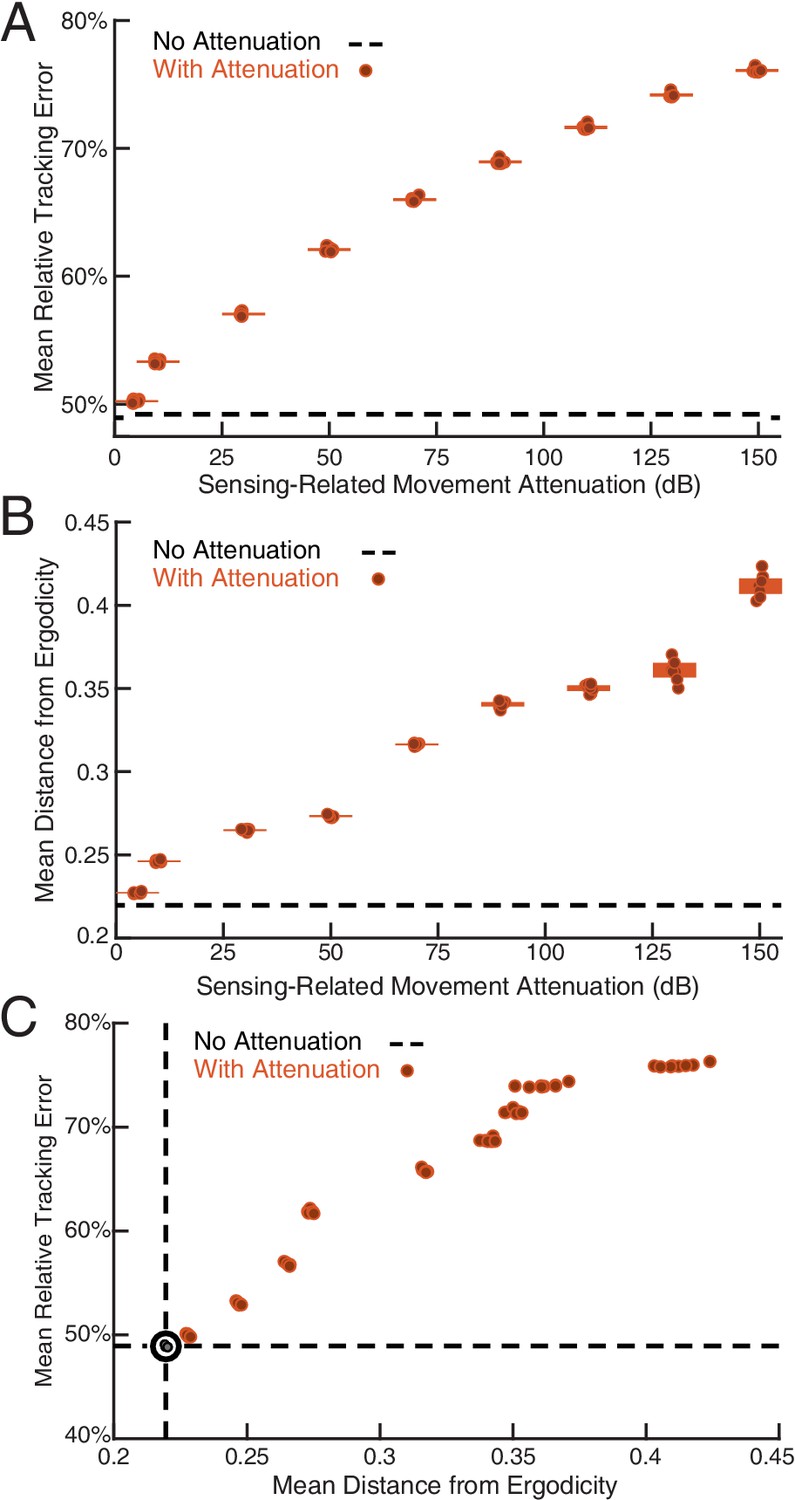
Sensing-related movements reduce tracking error.
The full-body oscillation in the simulated EIH weak signal sensor trajectory (similar to Figure 2H) was gradually removed through stepped increases of attenuation over the sensing-related movement frequency band (Materials and methods) with eight trials per condition (total ) to establish the confidence interval. (A) Relative tracking error (% of amplitude of the target’s fore-aft movement) as sensing-related movement is attenuated. The line near 50% error shows relative tracking error for the original unfiltered trajectory (0 dB attenuation). The thickness of the horizontal bars represents the 95% confidence interval across the eight trials (individual dots) for each attenuation condition. For each attenuation level, the individual trial dots are plotted with a small horizontal offset to enhance clarity. The baseline tracking error with no attenuation is marked by the dashed black line. (B) Distance from ergodicity (Materials and methods) as a function of sensing-related movement attenuation. Zero distance from ergodicity indicates the optimal trajectory that perfectly matches the statistics of the EID. As the distance increases from zero, the corresponding trajectory samples the EID further from the perfect proportional-betting ideal. The baseline data with no attenuation is marked by the dashed black line. (C) Relative tracking error plotted against distance from ergodicity across attenuation levels. There is a clear positive correlation between tracking error and distance from ergodicity as sensing-related movements are diminished.
Figure 4—figure supplement 1
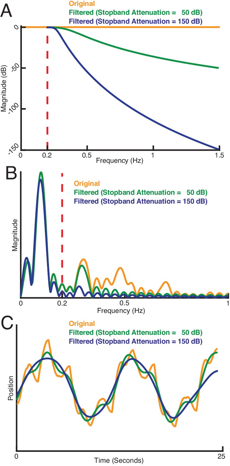
How sensing-related movements were attenuated for analyzing the impact of their diminishment.
(A) Response of three types of sensing-related movement attenuation filters. We used an IIR lowpass filter with a cutoff frequency of 0.2 Hz to avoid filtering the baseline tracking frequency band of the target (0.1 Hz in this case). In the two filtered examples shown, the attenuation at 1.5 Hz is set to 50 dB and 150 dB to achieve progressively stronger attenuation of sensing-related motion. (B) Frequency response of the original and filtered trajectory. The baseline tracking gain between 0 Hz to 0.2 Hz is well preserved while the sensing-related motion frequency band between 0.2 Hz to 1.5 Hz is attenuated according to the attenuation gain. (C) Comparison of original and filtered trajectories. As the stopband attenuation increases, the amplitude of sensing-related movements decrease.
Figure 5
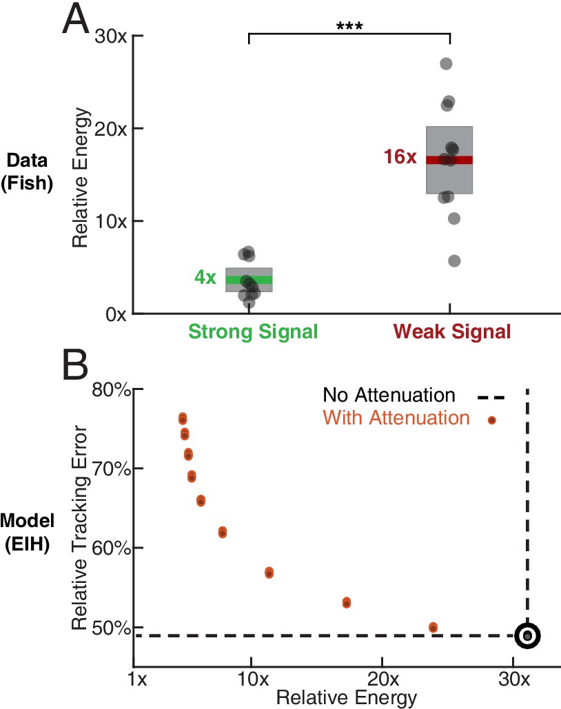
Relative energy for electric fish tracking behavior and EIH-generated behavior with attenuated body oscillations.
(A) Relative energy (definition: text) used by the electric fish during refuge tracking behavior under strong and weak signal conditions. Trials are similar to those shown in Figure 2C–D. Weak signal conditions show a significantly higher relative energy as a result of the additional sensing-related movements (Kruskal-Wallis test, , ). (B) Relative energy and relative tracking error for EIH simulations as sensing-related movements are progressively attenuated (data from Figure 4A–C, weak signal condition). As the sensing-related movements are attenuated, simulating investment of less mechanical effort for tracking, the relative energy decreases from 30x to less than 5x, but tracking error increases from 50% to around 75%. This plot suggests diminishing returns in tracking error reduction with additional energy expenditure beyond 30x. The lower bound near 4x is similar to the relative energy for the strong signal condition and arises due to small disparities from the sinusoid that the refuge is following (the 1x path). Asterisks indicate the range of values for the Kruskal-Wallis test (* for , ** for , and *** for ).
Figure 6 with 5 supplements
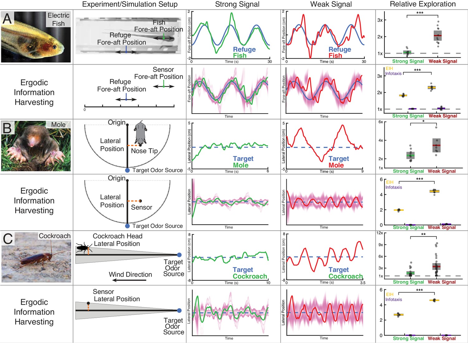
Trajectory comparison of animals tracking a target compared to EIH, and relative exploration across all trials.
Three representative live animal trajectories above trajectories generated by the EIH algorithm, with their duration cropped for visual clarity. The moth data is not shown here due to the complexity of the prescribed target motion, but is shown in a subsequent figure. All EIH simulations were conducted with the same target path as present in the live animal data, using a signal level corresponding to the weak or strong signal categories (Materials and methods). The EID is in magenta. Relative exploration across weak and strong signal trials (dots) is shown in the right-most column (solid line: mean, fill is 95% confidence intervals). Included for comparison is the relative exploration predicted by infotaxis (Vergassola et al., 2007). (A) The previously shown electric fish data to aid comparison to other species. As discussed, EIH agrees well with measured tracking behavior. Infotaxis (purple), in contrast, leads to hugging the edge of the EID, resulting in smooth pursuit behavior as indicated by the near 1x relative exploration. (B) The experimental setup and data for the mole was extracted from a prior study (Catania, 2013). During the mole’s approach to a stationary odor source, its lateral position with respect to the reference vector (from the origin to the target) was measured. Relative exploration was significantly higher under the weak signal conditions (Kruskal-Wallis test, , ). In the second row, raw exploration data (lateral distance traveled in normalized simulation workspace units) are shown to allow comparison to simulations, as the latter are done in 1-D (Materials and methods). EIH shows good agreement with significantly increased exploration for weak signal (Kruskal-Wallis test, , ), while infotaxis leads to cessation of movement. (C) The experimental setup and data for the cockroach was extracted from a prior study (Lockey and Willis, 2015). The cockroach head’s lateral position was tracked, and total travel distance was measured during the odor source localization task. Relative exploration is significantly higher for the weak signal condition (Kruskal-Wallis test, , ). In the second row, we show that EIH raw exploration (as defined above) agrees well with measurements as the amount of exploration increased significantly under weak signal conditions (Kruskal-Wallis test, , ), while infotaxis leads to cessation of movement. Asterisks indicate the range of values for the Kruskal-Wallis test (* for , ** for , and *** for ). Photo credit: Copyright Kirk, 2008; Eigenmannia image courtesy of Will Kirk, composite image composed and edited by Eric Fortune and Eatai Roth, under a CC BY 2.5 generic license.
© Catania, 2008. Mole image courtesy of Kenneth Catania. Published under a CC BY SA 3.0 unported license.
© Wikimedia Commons, 2013. Cockroach image courtesy of Wikimedia Commons. Published under a CC BY SA 3.0 unported license.
Figure 6—figure supplement 1
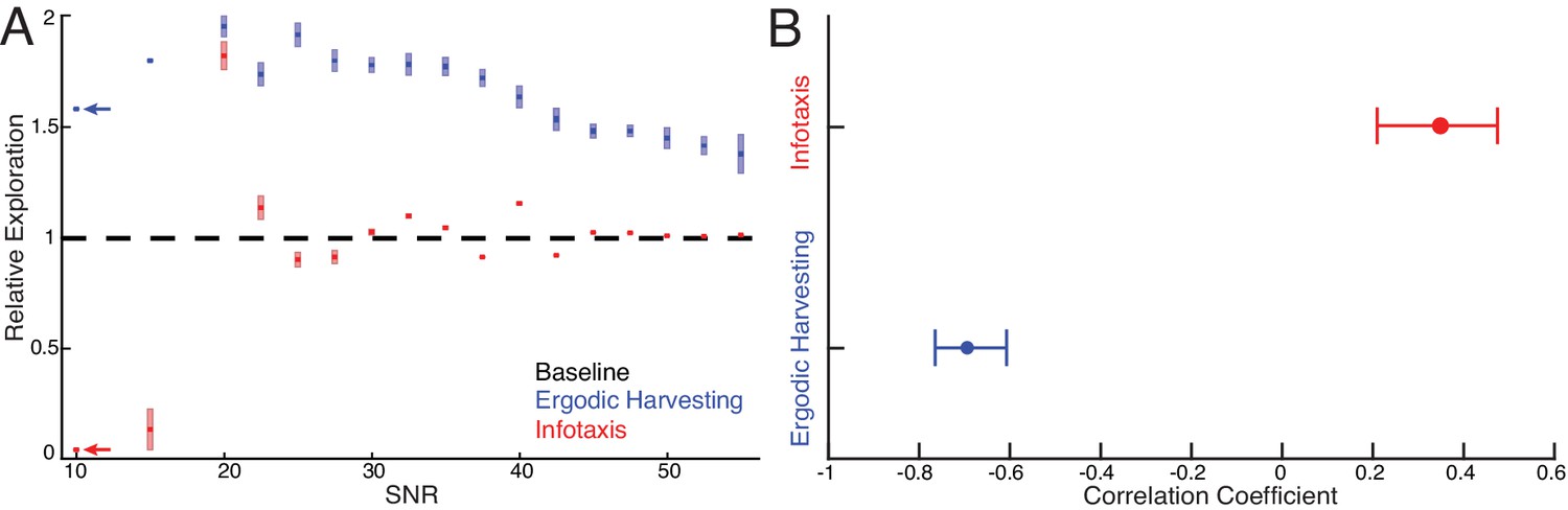
Systematic comparison between EIH and infotaxis in tracking a sinusoidally moving target.
Simulations of a sensor tracking a target moving sinusoidally under 17 different SNR conditions from 10 dB to 55 dB. For each SNR condition, 10 simulations with different pseudo-number seeds are performed to establish the confidence interval ( for EIH, for infotaxis). (A) As the SNR decreases from 55 dB, EIH exhibits elevated relative exploration (see Materials and methods) in the form of increased sensing-related movements. This is consistent with the animal behaviors summarized in Figures 1–7. EIH’s elevated exploration with decreasing SNR tapers at ≈20 dB as the Bayesian filter fails to converge the posterior due to significantly less informative measurements. Infotaxis does not show the trend of increased exploration as signal weakens between 55–20 dB and prescribed cessation of movement at the lowest (10 dB) signal strength. Throughout most of the frequency spectrum, infotaxis attempts to hug one edge of the EID, leading to near unity relative exploration. The increase in exploration at 20 dB is discussed in Appendix 6. (B) The correlation coefficient between relative exploration and signal strength computed from A for EIH and infotaxis (n = 170 trials for EIH, and n = 170 for infotaxis). The horizontal line indicates the 95% confidence interval. Ergodic harvesting has a significantly more negative correlation, indicating exploration increases as signal strength declines. The same trend is absent in infotaxis.
Figure 6—figure supplement 2
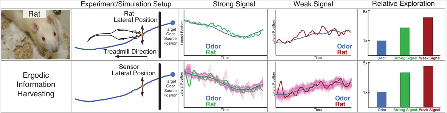
Rat odor tracking behavior and EIH simulation.
In a prior study (Khan et al., 2012), Wistar rats (Rattus norvegicus, Berkenhout 1769) performed an odor tracking task by following a uniform odor trail on a moving treadmill with only olfactory information, under two different surgical conditions: with one side of the nose blocked (single-side nostril stitching) and no blocking (sham stitching) as a control group. The experiment setup and tracked trajectory is shown in the top panel. Position data on the axis parallel to the treadmill were ignored, while positions on the perpendicular axis were recorded. The relative exploration was computed as with electric fish, using the cumulative 1D distance traveled by the rat divided by the cumulative distance of the transverse location of the odor trail. The olfactory system of the rat was modeled in the same fashion as for electric fish: as eventually providing an estimate of the location of the odor trail, modeled as a single 1D point-sensor of location with a Gaussian probability distribution controlled by the SNR of simulation (Materials and methods). The blocked nostril condition is here counted as the weak signal with lower SNR, and the sham stitching condition is counted as the strong signal. In the second row, we show EIH simulations of the weak and strong target trajectories, with the EID profile overlaid in magenta. It shows similar predicted sensor trajectories with a similar change in the relative exploration between these signal conditions as measured.
© Poirrier, 2007. Rat image courtesy of Jean-Etienne Minh-Duy Poirrier. Published under a CC BY SA 2.0 license.
Figure 6—figure supplement 3

Evolution of belief over time for the trials shown in Figure 6.
EIH simulations of tracking behavior of weakly electric fish, mole, and cockroach. The trials shown are identical to those shown in Figure 6. Simulated sensor position over time is the solid green line for the strong signal condition and the solid red line in the weak signal condition. The target position is the dashed black line. The repeated dashed gray lines mark each planning update event that segment the trajectory into individual planned trajectory segments of length T. The blue heatmap shows the progression of the belief over time. Note the presence of fictive distractors, where the belief distribution becomes multi-peaked (asterisks).
Figure 6—figure supplement 4

Sensitivity analysis on the ratio between control cost and ergodic cost in the objective function of trajectory optimization.
Simulations are conducted in the same way as Figure 6—figure supplement 1 but only for a fixed SNR under weak signal conditions (20 dB). The control cost prefactor R is varied while fixing the ergodic cost prefactor to be five for all the simulations. We simulated 16 different ratios of (shown along x axis on a log scale), each done with 10 different pseudo-random number seeds to establish confidence intervals. The relative exploration of the simulated trajectories are shown in the y axis on a linear scale with the sample mean marked by the solid color line and 95% confidence interval marked by the vertical color patch. The ratio used for all but the moth simulations included in the results is shown by the red dashed vertical line, while the moth ratio is shown by the orange dashed vertical line. Overall, as increases, relative exploration declines monotonically because movement incurs higher cost. The trend also suggests that as the ratio increases, movement will cease. The value of that we used across most of study results in a relative exploration value of around 2, with slightly lower relative exploration for the used for the moth simulations. The variation in relative exploration with an order of magnitude change in from 1 to 10 is approximately 2.5 to 1.5. The same sensitivity analysis was also done for a strong signal condition but is not shown as the trend is similar.
Figure 6—figure supplement 5
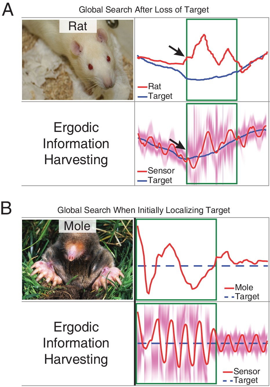
Measurements compared to prediction of EIH in two conditions where an animal needs to find the signal during tracking behavior.
As a demonstration of how our model seamlessly transitions between exploitation and exploration, we examined an instance in the measured behavior of the live animals in which the rat appears to lose a signal it is following (Khan et al., 2012) and an instance in which the mole starts off without finding the path to the source (Catania, 2013). The measured result shown here for both animals was wider casting motions transverse to the direction of movement. We examined whether these two behaviors (wider casting with loss of signal during tracking or when not finding the signal initially) would be predicted by EIH. (A) To simulate the condition of losing a signal trail in the middle of a successful tracking trial, we ran EIH as for the rat olfactory tracking case of Figure 6—figure supplement 2, but with the trajectory shown in in panel A. In the ‘target lost’ region (green square in figure), the sensor’s input was replaced by random draws from the observation model. (B) To simulate the condition of starting without knowing where the trail is for an extended period of time, we ran EIH as for the mole olfactory tracking case of Figure 6B, but with the trajectory shown in panel B. In the ‘target not yet acquired’ region (green square in figure), the sensor’s input was replaced by random draws from the observation model. In both instances, we observed wider casting motions transverse to the direction of travel similar to those measured (output from EIH below experimental data, overlaid with the EID profile in magenta). Similar to the measured behavior, our algorithm seamlessly transitions from exploitation to exploration when the expected information density becomes more diffuse.
© Poirrier, 2007. Rat image courtesy of Jean-Etienne Minh-Duy Poirrier. Published under a CC BY SA 2.0 license.
© Catania, 2008. Mole image courtesy of Kenneth Catania. Published under a CC BY SA 3.0 unported license.
Figure 7

Spectral analysis of live animal behavior and simulated behavior.
All the single trial Fourier spectra shown in A-B, E-F, and I-J are for the trials shown in Figure 6. (A–B) The already shown spectral analysis of the fish tracking data is included here for comparison, with target trajectory (blue), strong signal condition (green), and weak signal condition (red). The frequencies above the frequency domain of the target’s movement are shaded; components in the non-shaded region are excluded in the subsequent analysis. The Fourier magnitude is normalized. (C–D) The distribution of the mean normalized Fourier magnitude within the sensing-related movement frequency band (gray shaded region) for strong and weak signal trials, as shown before. (E–F) Representative Fourier spectra of the measured and modeled head movement of a mole while searching for an odor source (lateral motion only, transverse to the line between origin and target), plotted as in A-B. Because the target is stationary in contrast to the fish data, the entire frequency spectrum was analyzed. (G–H) Mean Fourier magnitude distribution, normalized to the strong signal condition to emphasize difference between the strong and weak cases. In the weak signal condition, there is significantly more lateral movement power under weak signal in both the animal data and simulation (Kruskal-Wallis test, , for behavior data, and , for EIH simulations). (I–J) Fourier spectra of mole’s lateral trajectory, plotted the same as in A-B. (K–L) Mean Fourier magnitude distribution. Significantly higher power is found under weak signal in the behavior data and simulations (Kruskal-Wallis test, , for behavior data, and , for EIH simulations). (M–N) Bode magnitude plot (Materials and methods) of a moth tracking a robotic flower that moves in a sum-of-sine trajectory (figure adapted from Stöckl et al., 2017) and the corresponding simulation using the same target trajectory. Each dot in the Bode plot indicates a decomposed frequency sample from the first 18 prime harmonic frequency components of the flower’s sum-of-sine trajectory. A total of 23 trials ( for strong signal, and for weak signal) were used to establish the 95% confidence interval shown in the colored region. Note the increase in gain in the midrange frequency region (shaded in gray) between the strong signal and weak signal conditions. The confidence interval for the simulation Bode plot is established through 240 trials ( for strong signal, and for weak signal). The same midrange frequency regions (shaded in gray) are used for the subsequent analysis. (O–P) Mean midrange frequency tracking gain distribution for the moth behavior and simulation trials. Moths exhibit a significant increase in midrange tracking gain for the weaker signal condition (Kruskal-Wallis test, , ), in good agreement with simulation (Kruskal-Wallis test, , ). Asterisks indicate the range of values for the Kruskal-Wallis test (* for , ** for , and *** for ).
Videos
Video 1
Segments of behavior across the four species analyzed.
Video 2
The ergodic information harvesting algorithm applied to stationary object localization in a bio-inspired electrolocation robot.
Tables
Table 1
Parameters of EIH Simulation.
| Parameter | Symbol | Value | Source and note |
|---|---|---|---|
| Variance of observation model | 0.06 | is initially chosen to fit weakly electric fish behavior and kept the same for all the sensory modalities simulated for the sake of model consistency | |
| Time step of the simulation | 0.025, 0.005 | In seconds. is initially chosen to fit weakly electric fish behavior and fixed for all the EIH and infotaxis simulations except for moth, where is set to 0.005 s to account for the higher velocity of the sum-of-sine trajectory | |
| Duration of planned trajectory | T | 2.5, 0.5 | In seconds. T is initially chosen to fit weakly electric fish behavior and kept the same for all the EIH simulations except for moth, where T is set to 0.5 to account for the higher velocity of the sum-of-sine trajectory |
| Step size control of the backtracking line search of trajectory optimization | 0.1 | and are picked to balance between the speed of convergence and the final cost of the trajectory optimization and are fixed across all the EIH simulations | |
| Step size control of the backtracking line search of trajectory optimization | 0.4 | and are picked to balance between the speed of convergence and the final cost of the trajectory optimization and are fixed across all the EIH simulations | |
| Weight of the distance from ergodicity term in the cost function of trajectory optimization loop (see Algorithm 1) | 5 | is initially chosen to fit weakly electric fish behavior and kept the same for all the simulations. Note that changing changes the trade-off between distance from ergodicity (how much information one wants) and control effort (how much energy one is willing to give up). As a result, there is mild sensitivity to this parameter—making it an order of magnitude larger will lead to a more exploratory trajectory while making it an order of magnitude smaller will lead to less exploration. If is set to zero, no movement will occur at all. For further discussion of this point, see Miller et al., 2016. Finally, a sensitivity analysis is also provided in Figure 6—figure supplement 4 | |
| Weight of the control term in the cost function of trajectory optimization loop (see Algorithm 1) | R | 10, 20 | R is initially chosen to fit weakly electric fish behavior and kept the same for all the simulations except for moth, where R is set to 20 since otherwise, the simulated moth body moves faster than the measured data due to the decrease in T from 2.5 to 0.5. Note that the control cost is equivalent to the total kinetic energy required to execute the candidate trajectory given our assumption of a unit point-mass body |
| Number of dimensions used for Sobolev space norm in ergodic metric | 15 | is initially chosen to be a sufficient number for representing all the behavioral data considered in this paper and kept the same for all the simulations | |
| Initial control input | 0 | Zero control is applied at the beginning of every simulation | |
| Initial belief | Initial belief is set and fixed to a uniform (“flat”) prior distribution within the workspace (from 0 to 1) where the probability of the target being at every location is identical |
Table 2
Simulation parameters used for each figure.
| Figure | Category | SNR (dB) | Initial position | Target trajectory | Biological condition |
|---|---|---|---|---|---|
| Figure 1E | Weak Signal | ≤30 | 0.7 | Sinusoid | N/A (simulation) |
| Figure 1F | Strong Signal | ≥50 | 0.7 | Sinusoid | N/A (simulation) |
| Figure 2G,I and 3A-C | Weak Signal | ≤30 | 0.4 | Sinusoid | N/A (simulation) |
| Figure 2F,H and 3A-C | Strong Signal | ≥50 | 0.4 | Sinusoid | N/A (simulation) |
| Figure 2—figure supplement 1 | Weak Signal | ≤30 | 0.4 | Stationary | N/A (simulation) |
| Figure 2—figure supplement 2 | Weak Signal | ≤30 | 0.4 | Stationary | N/A (simulation) |
| Figure 4A–C and Figure 5B | Weak Signal | ≤30 | 0.4 | Sinusoid | N/A (simulation) |
| Figure 6A and Figure 7B,D | Strong Signal | ≥50 | 0.4 | Sinusoid | No jamming |
| Figure 6A and Figure 7B,D | Weak Signal | ≤30 | 0.4 | Sinusoid | mA jamming |
| Figure 6B and 7F,H | Strong Signal | ≥50 | 0.2 | Stationary | Intact control |
| Figure 6B and 7F,H | Weak Signal | ≤30 | 0.6 | Stationary | Single-side nostril block and crossed airflow |
| Figure 6C and 7J,L | Strong Signal | ≥50 | 0.475 | Stationary | 4 mm intact antenna |
| Figure 6C and 7J,L | Weak Signal | ≤30 | 0.4 | Stationary | 1 and 2 mm bilaterally trimmed antenna |
| Figure 6—figure supplement 1 | Strong and Weak Signal | 10–55 | 0.4 | Sinusoid | N/A (simulation) |
| Figure 6—figure supplement 2 | Strong Signal | ≥50 | 0.8 | Prescribed by study (Khan et al., 2012) | Sham stitching |
| Figure 6—figure supplement 2 | Weak Signal | ≤30 | 0.3 | Prescribed by study (Khan et al., 2012) | Single-side nostril stitching |
| Figure 6—figure supplement 3 | Strong Signal | ≥50 | 0.4 | Sinusoid | N/A (simulation) |
| Figure 6—figure supplement 3 | Weak Signal | ≤30 | 0.4 | Sinusoid | N/A (simulation) |
| Figure 6—figure supplement 4 | Weak Signal | 20 | 0.4 | Sinusoid | N/A (simulation) |
| Figure 6—figure supplement 5A | Weak Signal | ≤30 | 0.9 | Prescribed by study (Khan et al., 2012) | Single-side nostril stitching |
| Figure 6—figure supplement 5B | Weak Signal | ≤30 | 0.45 | Stationary | Single-side nostril block |
| Figure 7N,P | Strong Signal | ≥50 | 0.4 | Prescribed by study (Stöckl et al., 2017) | 3000 lux ‘high-light’ |
| Figure 7N,P | Weak Signal | ≤30 | 0.4 | Prescribed by study (Stöckl et al., 2017) | 15 lux ‘low-light’ |
Additional files
Download links
A two-part list of links to download the article, or parts of the article, in various formats.
Downloads (link to download the article as PDF)
Open citations (links to open the citations from this article in various online reference manager services)
Cite this article (links to download the citations from this article in formats compatible with various reference manager tools)
Tuning movement for sensing in an uncertain world
eLife 9:e52371.
https://doi.org/10.7554/eLife.52371


