Figures and data in Hierarchical temporal prediction captures motion processing along the visual pathway

Figures
Tables
Additional files

9 figures, 1 table and 1 additional file

Figures

Figure 1 with 1 supplement

Download asset Open asset

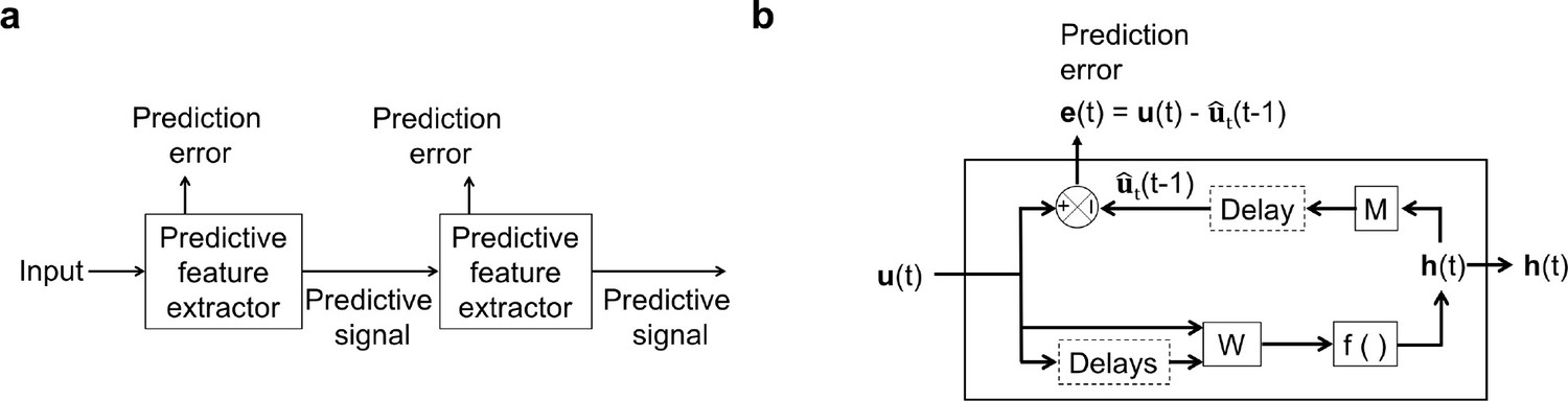
An illustration of the general architecture of the hierarchical temporal prediction model.

(a) Architecture of the hierarchical temporal prediction model. Each stack of the model (labeled ‘predictive feature extractor’) receives input from the stack below and finds features of its input that are predictive of its future input, with the lowest stack predicting the raw natural inputs. The predictive signal is fed forward to the next layer. (b) Operations performed by each stack of the temporal prediction model. Each stack receives a time-varying input vector $u (t)$ , which in all but the first stack is the hidden unit activity vector $h (t)$ from the lower stack. For the first stack, the input $u (t)$ is raw visual input (i.e. video). The input, also with some additional delayed input, passes through feedforward input weight matrix $W$ and undergoes a nonlinear transformation $f ()$ to generate hidden unit activity $h (t)$ . Each stack is optimized so that a linear transformation $M$ from its hidden unit activity $h (t)$ , and then a delay, generates an accurate estimate ${\hat{u}}_{t} (t - 1)$ of its future input (at time $t$ ). Because of the delay, the predicted input is in the future relative to the input that generated the hidden unit activity. This delay is shown at the end of processing, but is likely distributed throughout the system. For each stack, the prediction error is only used to train the input and output weights $W$ and $M$ . The prediction error can equivalently be written as $e (t + 1) = u (t + 1) - {\hat{u}}_{t + 1} (t)$ . To see how this hierarchical temporal prediction model differs from predictive coding (Rao and Ballard, 1999) and PredNet (Lotter et al., 2020) see Figure 1—figure supplement 1.

Figure 1—figure supplement 1

Download asset Open asset

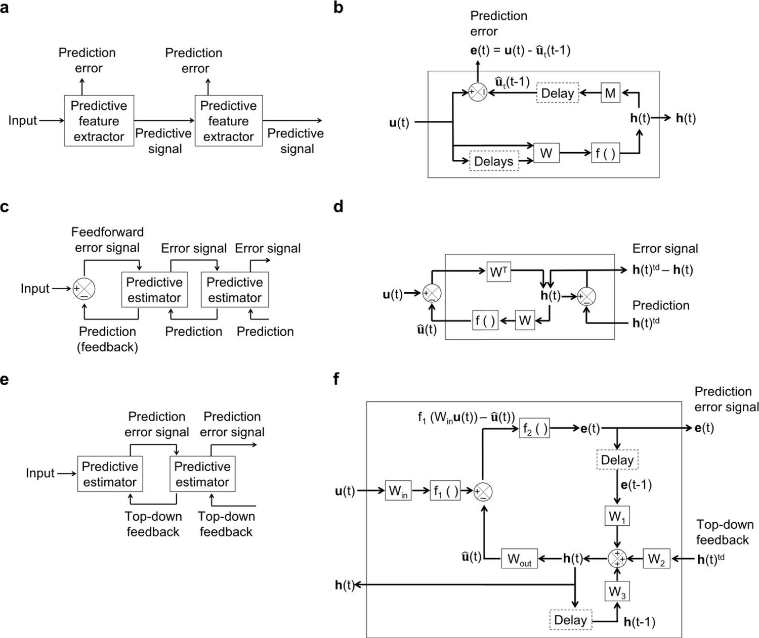
Architecture and operations performed by temporal prediction, predictive coding and PredNet models.

(a) Architecture of the hierarchical temporal prediction model. Each stack of the model (labeled ‘predictive feature extractor’) receives input from the stack below and finds features of its input that are predictive of its future input, with the lowest stack predicting the raw natural inputs. The predictive signal is fed forward to the next layer. (b) Operations performed by each stack of the temporal prediction model. See the caption of Figure 1 for more details. (c) General architecture of Rao and Ballard, 1999 hierarchical predictive coding model. At each layer (labeled ‘predictive estimator’), the model generates an estimate of its input which is fed back down to the previous layer. Top-down predictions from the layer above are subtracted from the current estimate and the error signal is fed forward to the next layer. (d) Operations performed at each layer of Rao and Ballard’s predictive coding model. The input $u (t)$ undergoes a linear transformation $W^{⊺}$ to generate hidden unit representation $h (t)$ . This is used to generate an estimate $\hat{u} (t)$ of the input at the same time step. An error neuron computes the difference between the hidden representation $h (t)$ and its estimate $h (t)^{t d}$ from the layer above. This error is passed forward as input to the next layer. (e), General architecture of the PredNet model (Lotter et al., 2016). At each layer, the model takes in the prediction error from the previous layer as input, with the bottom layer receiving the raw video frame. This layer then tries to predict the future of this input given the past error signal, past hidden unit activity and top-down input from the layer above. The prediction error (between the true future input and the model’s estimate of the input) are fed forward to the next layer, which in turn attempts to predict its future in the same manner. The layer above feeds back its hidden unit activity to the layer below. (f) Operations performed by each layer (labeled ‘Predictive estimator’ in (e)) of the PredNet model. In brief, the model receives a time-varying input $u (t)$ , which at the lowest layer is the raw video input and at all other layers is the prediction error from the layer below. The model then generates a hidden representation $h (t)$ from a combination of the prediction error at the previous time-step $e (t - 1)$ , the hidden representation at the previous time-step $h (t - 1)$ and the current hidden unit activity in the layer above $h (t)^{t d}$ . This hidden unit activity is used to generate a prediction $\hat{u} (t)$ of the input $u (t)$ , which is in the future relative to the past hidden unit activity and prediction error. The prediction error $e (t)$ is fed forward to the next layer, where it serves as the input to be predicted. The hidden unit activity $h (t)$ is fed down to the layer below, where it becomes $h (t)^{t d}$ . (**c, d**) adapted from Rao and Ballard, 1999.

Figure 2

Download asset Open asset

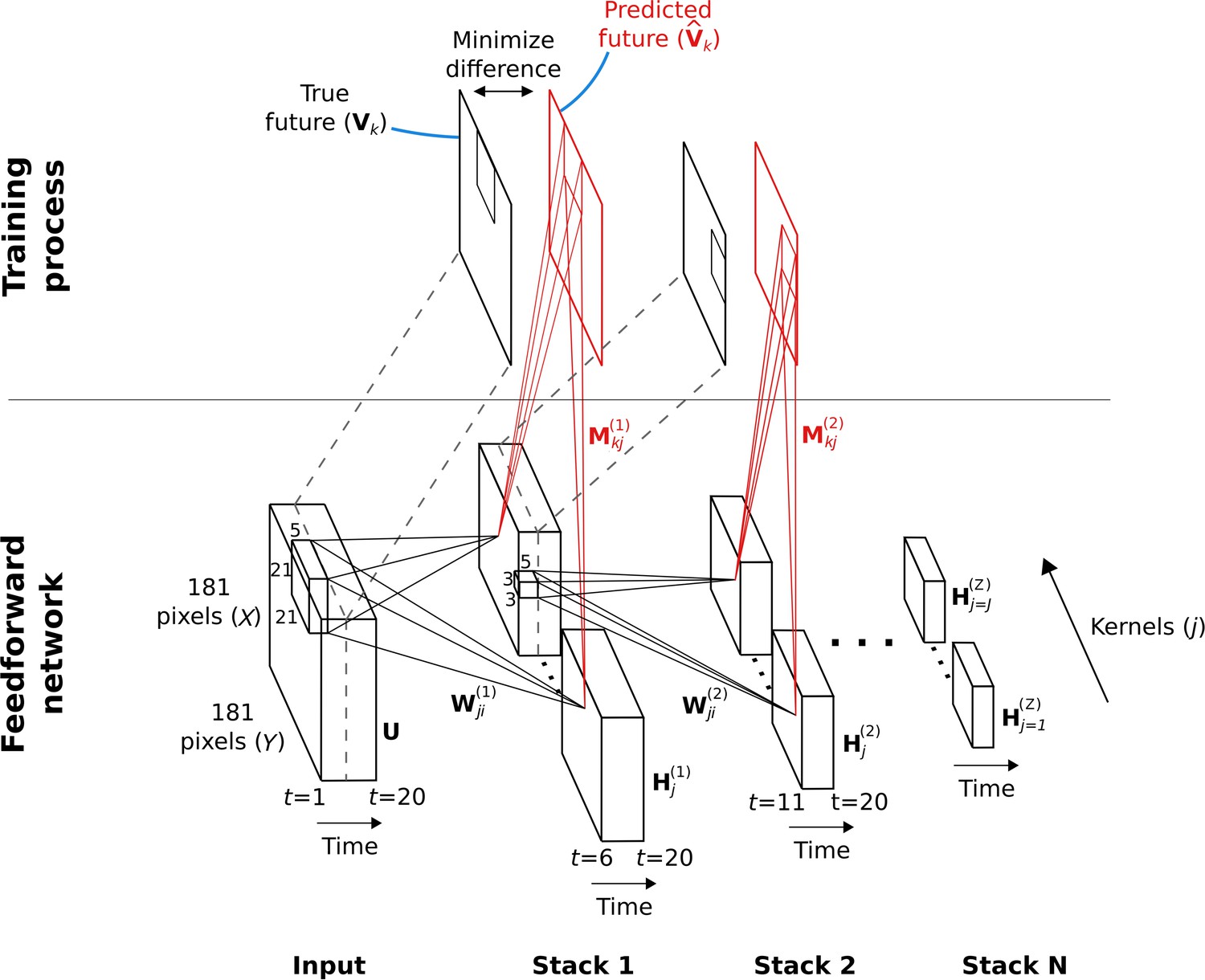
Hierarchical temporal prediction model in detail, with convolution.

Schematic of model architecture, illustrating the stacking and convolution. This model is essentially the same as the model in Figure 1 but using convolutional networks; the notation used here is slightly different from Figure 1 due to this. Each stack is a single hidden-layer feedforward convolutional network, which is trained to predict the future time-step of its input from the previous 5 time-steps. Each stack consists of a bank of $J$ convolutional hidden units, where a convolutional hidden unit is a set of hidden units that each have the same weights (the same convolution kernels). The first stack is trained to predict future pixels of natural video inputs, $U$ , from their past. Subsequent stacks are trained to predict future time-steps of the hidden-layer activity in the stack below, $H$ , based on their past responses to the same natural video inputs. For each convolutional hidden unit $j$ in a stack, its input $U_{i}$ from convolutional hidden unit $i$ in the stack below is convolved with an input weight kernel $W_{j i}$ , summed over $i$ , and then rectified, to produce its hidden unit activity $H_{j}$ . This activity is next convolved with output weight kernels $M_{k j}$ and summed over $j$ to provide predictions ${\hat{V}}_{k}$ of the immediate future input $V_{k}$ of each convolutional hidden unit, $k$ , in the stack below. Note, $V_{k}$ is just $U_{i}$ shifted one time step into the future, with $k = i$ . The weights ( $W$ , $M$ ) of each stack are then trained by backpropagation to minimize the difference between the predicted future ${\hat{V}}_{k}$ and the true future, $V_{k}$ . Each stack is trained separately, starting with the lowest stack, which, once trained, provides input for the next stack, which is then trained, and so on. The input and hidden stages of all the stacks when stacked together form a deep feedforward network. Note, to avoid clutter, only one time slice ${\hat{V}}_{k}$ and $V_{k}$ are shown. In the convolution model presented here, every bold capitalized variable is a 3D-tensor over space ( $x$ ), space ( $y$ ) and time ( $t$ ), and every italicized variable is a scalar, either a real number or an integer. The bracketed superscript on variables denotes the stack number $z$ up to top stack $Z$ .

Figure 3

Download asset Open asset

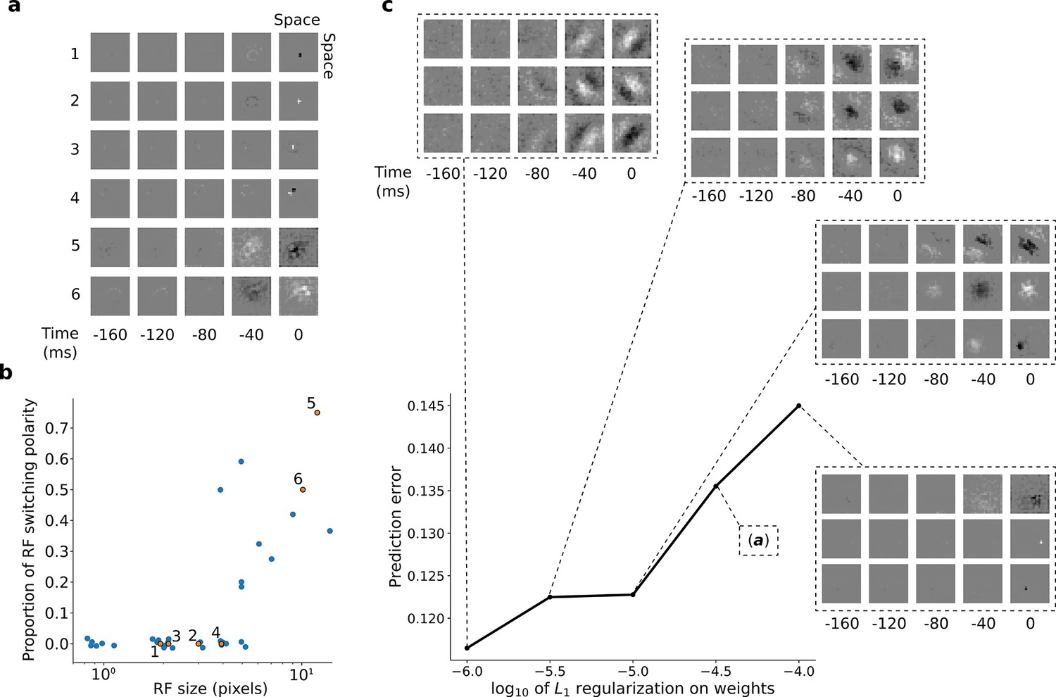
RFs of trained first stack of the model show retina-like tuning.

(a) Example RFs with center-surround tuning characteristic of neurons in retina and LGN. RFs are small and do not switch polarity over time (units 1–4) or large and switch polarity (units 5–6), resembling cells along the parvocellular and magnocellular pathways, respectively. (b) RF size plotted against proportion of the weights (pixels) in the RF that switch polarity over the course of the most recent two timesteps. Units in a labeled and shown in orange. (c) Effect of changing regularization strength on the qualitative properties of RFs.

Figure 4 with 1 supplement

Download asset Open asset

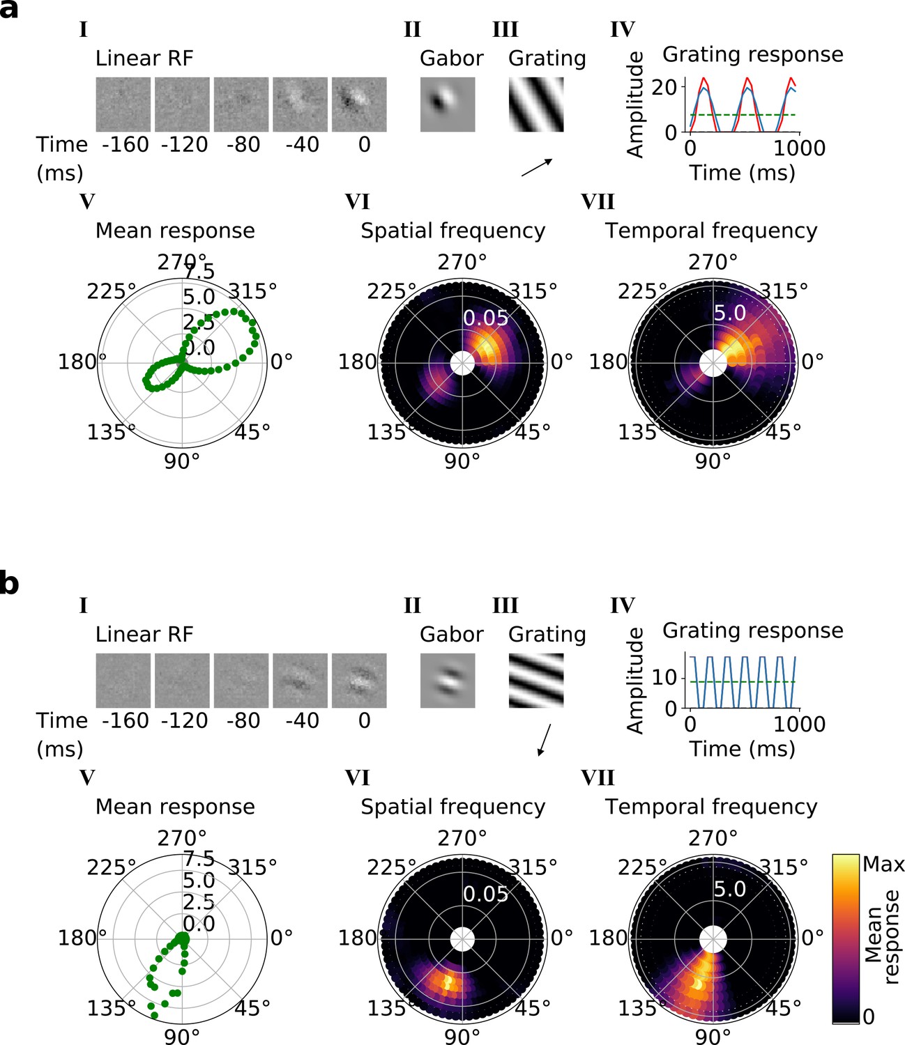
Qualitative tuning properties of example model units in stack 2.

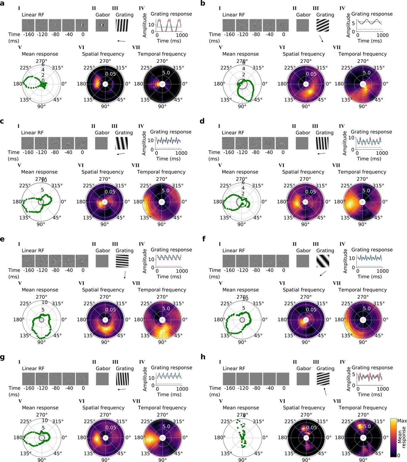
(**a, b**) Tuning properties of two example units from the 2nd stack of the model, including (I) the linear RF and (II) the Gabor fitted to the most recent time-step of the linear RF. (III) the drifting grating that best stimulates this unit. (IV) the amplitude of the unit’s response to this grating over time. Red line: unit response; blue line: best-fitting sinusoid; gray dashed line: response to blank stimulus, which is zero and hence obscured by the x-axis. Note that the response (red line) is sometimes obscured by a perfectly overlapping best-fitting sinusoid (blue line). (V) The unit’s mean response over time plotted against orientation (in degrees) for gratings presented at its optimal spatial and temporal frequency. (VI,VII) Tuning curves showing the joint distribution of responses to (VI) orientation (in degrees) and spatial frequency (in cycles/pixel) at the preferred temporal frequency and to (VII) orientation and temporal frequency (in Hz) at the preferred spatial frequency. In VI and VII the color represents the mean response over time to the grating presented. For more example units, see Figure 4—figure supplement 1.

Figure 4—figure supplement 1

Download asset Open asset

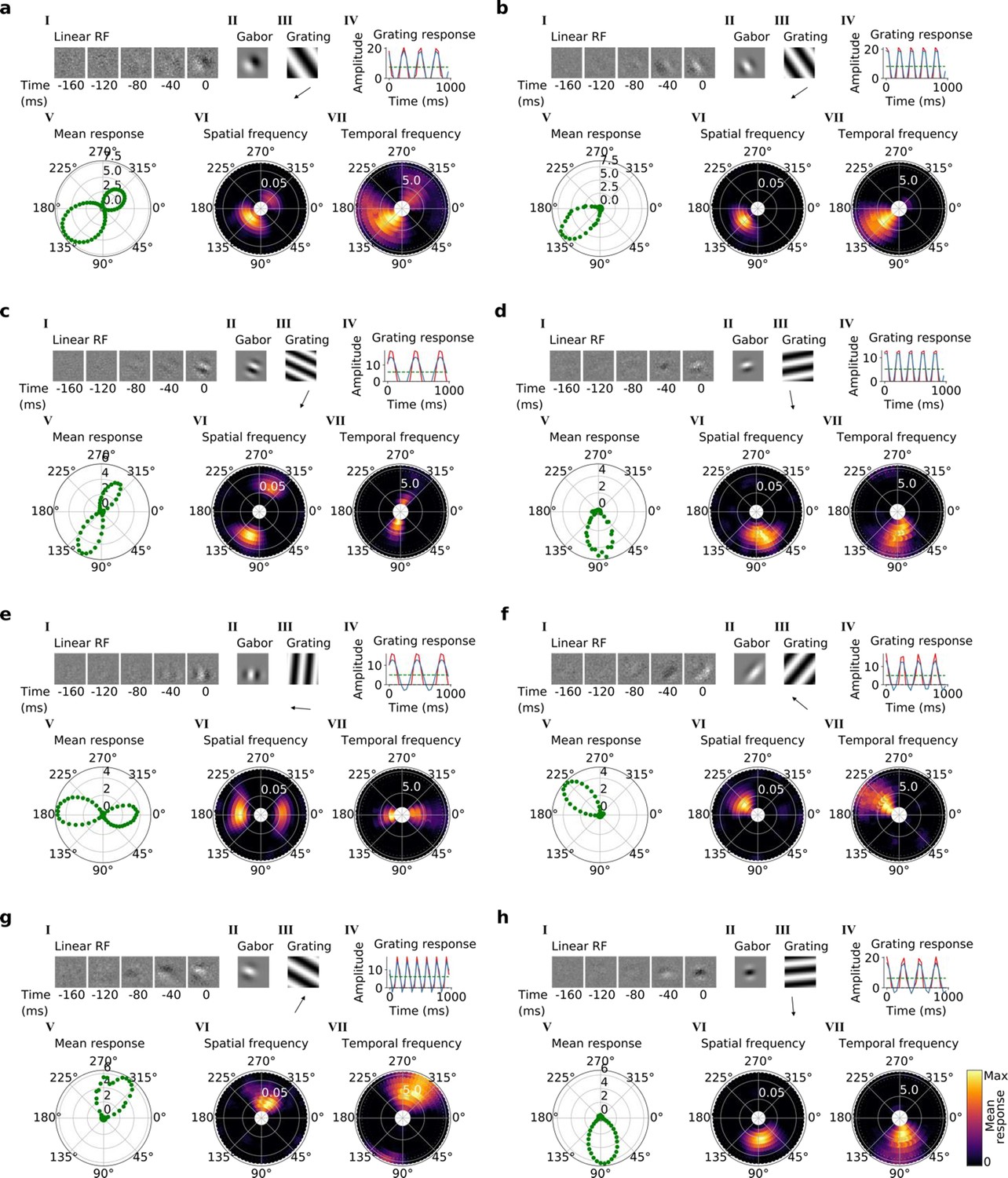
Tuning properties of example units in stack 2.

(**a–h**), I-VII as in Figure 4a and b.

Figure 5 with 2 supplements

Download asset Open asset

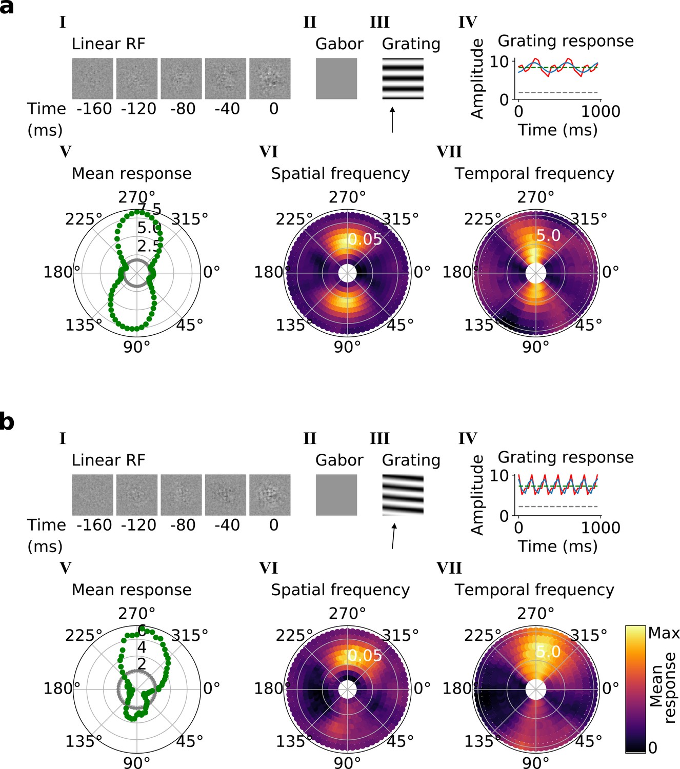
Qualitative tuning properties of example model units in stack 3.

(**a, b**), As in Figure 4a and b. Note that a(II) and b(II) when blank indicate that a Gabor could not be well fitted to the RF. Also, note that in a(IV) and b(IV) the response to a blank stimulus is visible as a gray line, whereas in the corresponding plots in Figure 4 this response is zero. For more example units, see Figure 5—figure supplement 1. Example units from stack 4 are shown in Figure 5—figure supplement 2.

Figure 5—figure supplement 1

Download asset Open asset

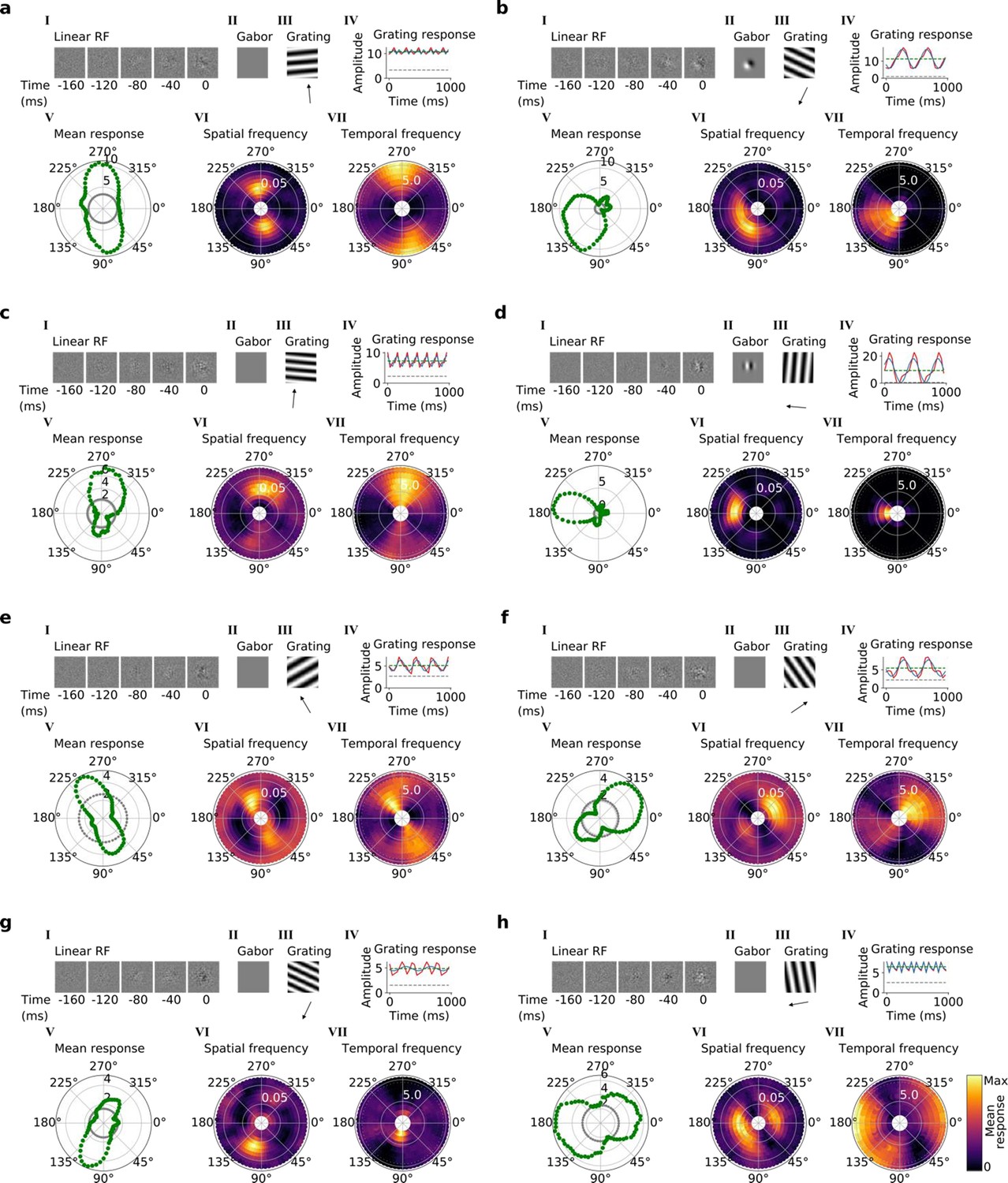
Tuning properties of example units in stack 3.

(**a–h**), I-VII as in Figure 4a and b.

Figure 5—figure supplement 2

Download asset Open asset

Tuning properties of example units in stack 4.

(**a–h**), I-VII as in Figure 4a and b.

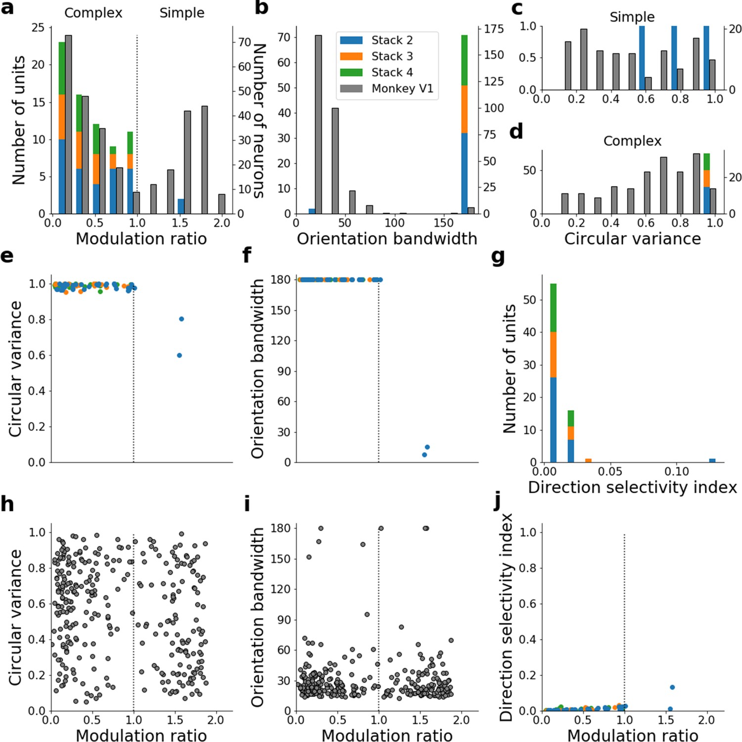
Figure 6 with 6 supplements

Download asset Open asset

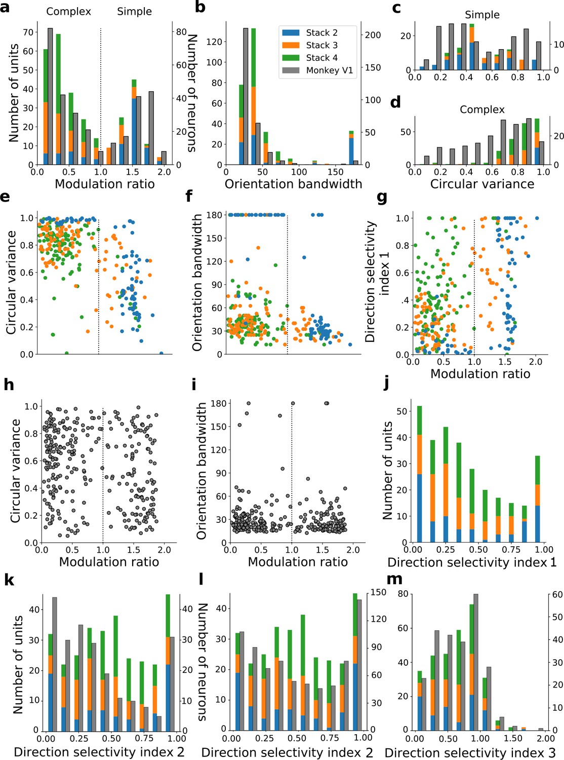
Quantitative tuning properties of model units in stacks 2–4 in response to drifting sinusoidal gratings and corresponding measures of macaque V1 neurons.

(**a–d**) Histograms showing tuning properties of model and macaque V1 (Ringach et al., 2002) neurons as measured using drifting gratings. Units from stacks 2–4 are plotted on top of each other to also show the distribution over all stacks; this is because no stack can be uniquely assigned to V1. Modulation ratio measures how simple or complex a cell is; orientation bandwidth and circular variance are measures of orientation selectivity. (**e, f, g**) Joint distributions of tuning measures for model units. (**h, i**) Joint distributions of tuning measures for V1 data; note similarity to e and f. (j) Distribution of direction selectivity for model units (using direction selectivity index 1, see Methods). (**k,l**) Distribution of direction selectivity for model units and macaque V1 (k from De Valois et al., 1982; l from Schiller et al., 1976) using direction selectivity index 2. (m) Distribution of direction selectivity for model units and for cat V1 (from Gizzi et al., 1990) using direction selectivity index 3. In all cases, for units with modulation ratios >1, only units whose linear RFs could be well fitted by Gabors were included in the analysis. To see the spatial RFs of these units and their Gabor fits, see Figure 6—figure supplement 1, and for those units not well fitted by Gabors see Figure 6—figure supplement 2. Some units had very small responses to drifting gratings compared to other units in the population. Units whose mean response was <0.1% of the maximum for the population were excluded from analysis. To see the RFs and Gabor fits and quantitative properties of the units of the present-predicting and the weight-shuffled control models, see Figure 6—figure supplements 3–6.

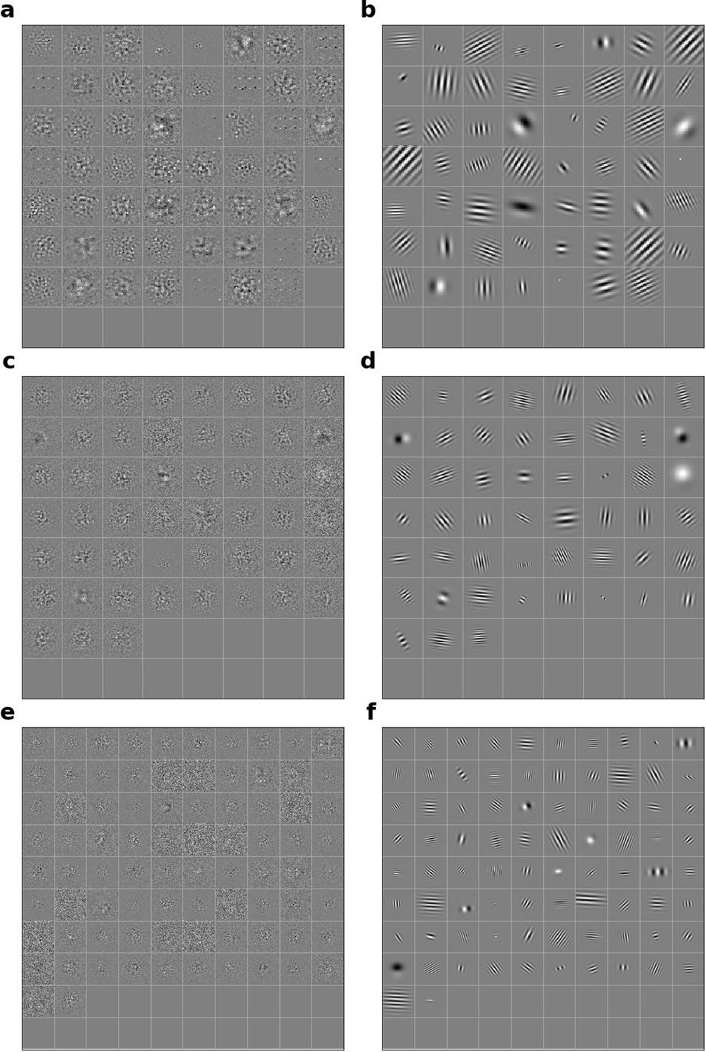
Figure 6—figure supplement 1

Download asset Open asset

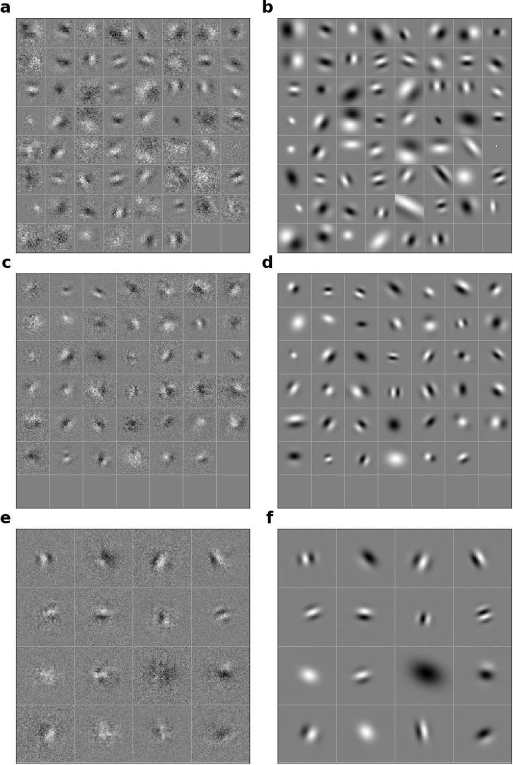
Linear RFs of model units that could be well fitted by Gabors and corresponding Gabors.

(a), Most recent time-step of linear RFs of model units in stack 2. (b), Corresponding Gabor fits to each RF shown in a. (**c, d**) as in a,b for units in stack 3. (**e, f**) as in a,b for units in stack 4.

Figure 6—figure supplement 2

Download asset Open asset

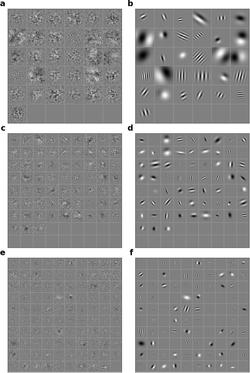
Linear RFs of model units that could not be well fitted by Gabors and corresponding Gabors.

(a), Most recent time-step of linear RFs of model units in stack 2. (b), Corresponding Gabor fits to each RF shown in a. (**c, d**) as in a,b for units in stack 3. (**e, f**) as in (**a,b**) for units in stack 4.

Figure 6—figure supplement 3

Download asset Open asset

Linear RFs of model units and corresponding Gabors for stacked autoencoding (present-predicting) model.

(a) Most recent time-step of linear RFs of model units in stack 2. (b) Corresponding Gabor fits to each RF shown in a. (**c, d**) as in a,b for units in stack 3. (**e, f**) as in a,b for units in stack 4.

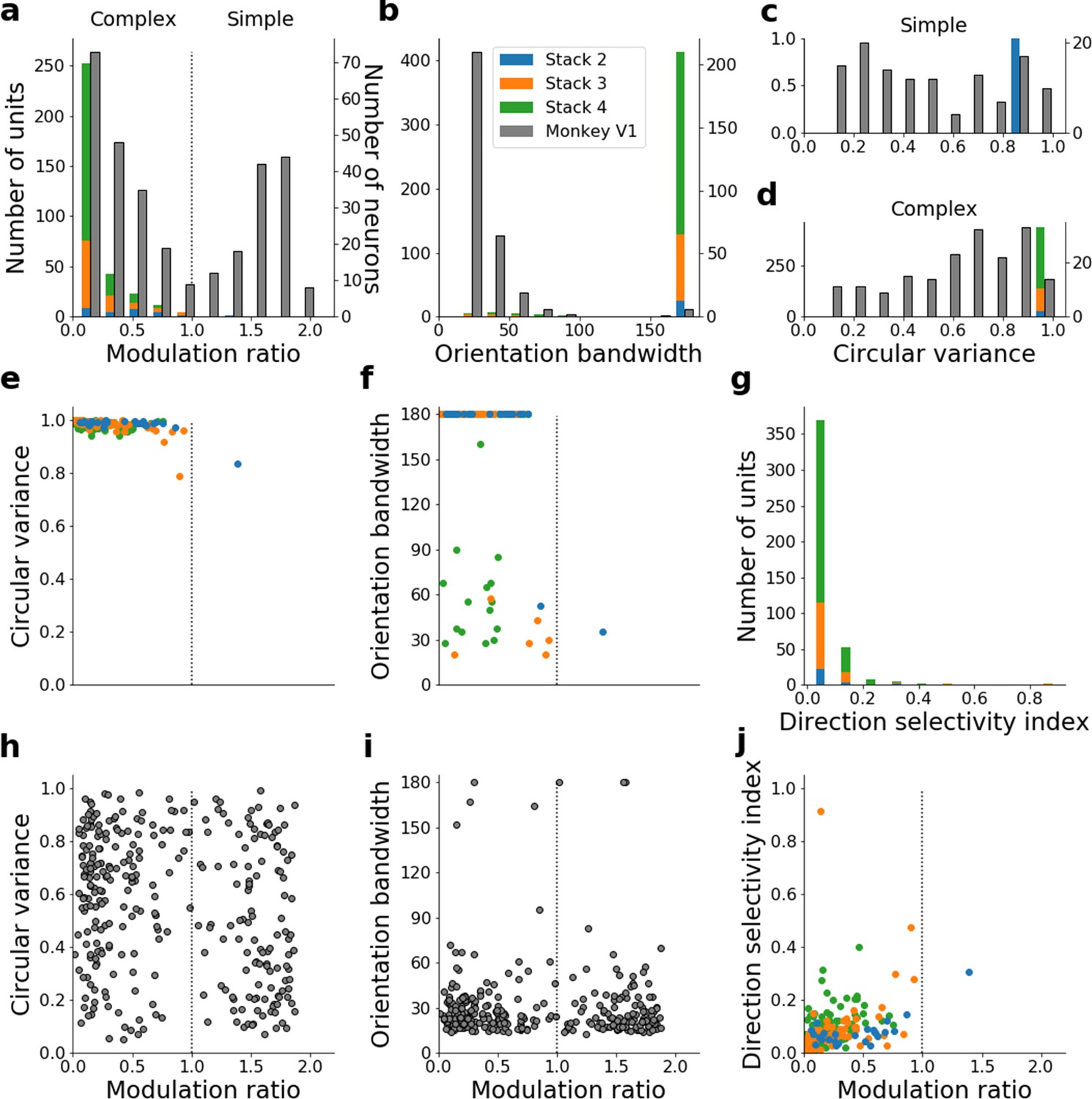
Figure 6—figure supplement 4

Download asset Open asset

Quantitative tuning properties of stacked autoencoding (present-predicting) model units in stacks 2–4 in response to drifting sinusoidal gratings and corresponding measures of macaque V1 neurons.

(**a–d**) Histograms showing tuning properties of model and macaque V1 neurons as measured using drifting gratings. Units from stacks 2–4 are plotted on top of each other to also show the distribution over all stacks; this is because no stack can be uniquely assigned to V1. Modulation ratio measures how simple or complex a cell is; orientation bandwidth and circular variance are measures of orientation selectivity. (**e, f**) Joint distributions of tuning measures for model units. (g) Distribution of direct selectivity for model units. (**h, i**) Joint distributions of tuning measures for V1 data; note similarity to e and f. (j) Joint distribution of direction selectivity and modulation ratio for model units.

Figure 6—figure supplement 5

Download asset Open asset

Linear RFs of model units and corresponding Gabors for the model with the input weights to each unit in the network shuffled across space and time.

(a) Most recent time-step of linear RFs of model units in stack 2. (b) Corresponding Gabor fits to each RF shown in a. (**c, d**) as in a,b for units in stack 3. (**e, f**) as in a,b for units in stack 4.

Figure 6—figure supplement 6

Download asset Open asset

Quantitative tuning properties of the model with input weights to each unit shuffled across space and time for units in stacks 2–4 in response to drifting sinusoidal gratings and corresponding measures of macaque V1 neurons.

(**a–d**) Histograms showing tuning properties of model and macaque V1 neurons as measured using drifting gratings. Units from stacks 2–4 are plotted on top of each other to also show the distribution over all stacks; this is because no stack can be uniquely assigned to V1. Modulation ratio measures how simple or complex a cell is; orientation bandwidth and circular variance are measures of orientation selectivity. (**e, f**) Joint distributions of tuning measures for model units. (g) Distribution of direct selectivity for model units. (**h, i**) Joint distributions of tuning measures for V1 data; note similarity to e and f. (j) Joint distribution of direction selectivity and modulation ratio for model units.

Figure 7

Download asset Open asset

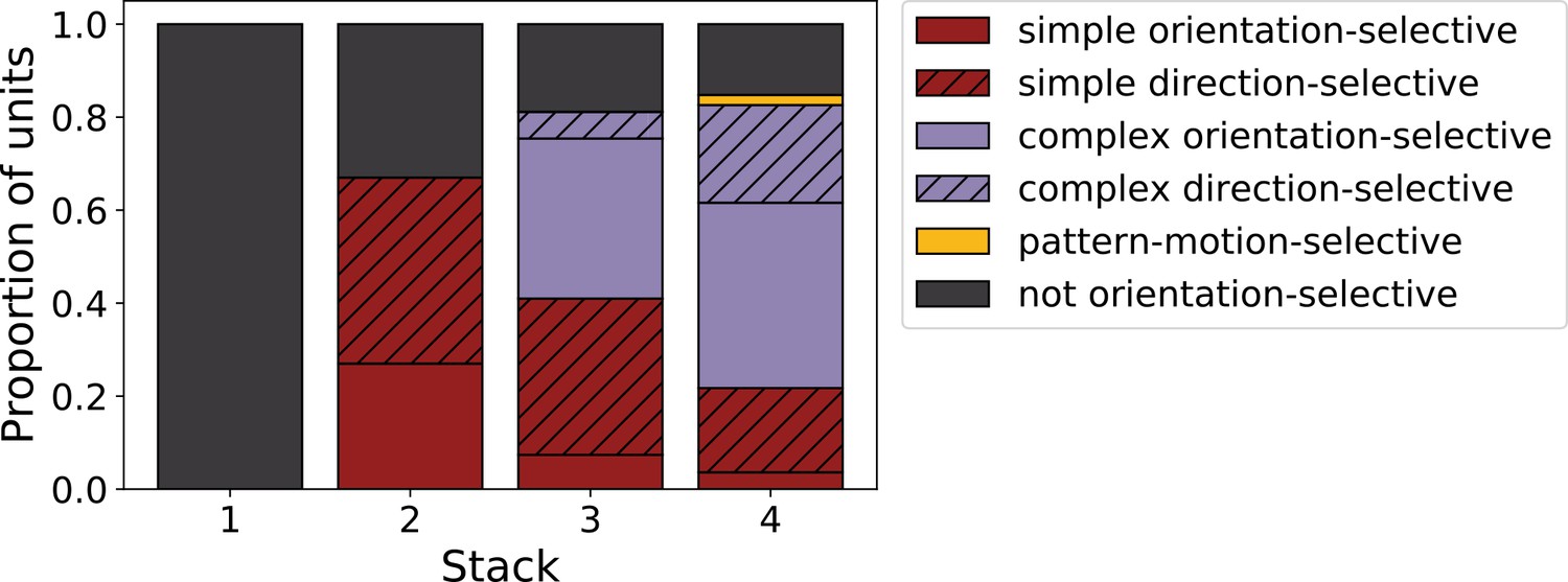
Progression of tuning properties across stacks of the hierarchical temporal prediction model.

Proportion of simple (red), complex (purple) and non-orientation-selective (gray) units in each stack of the model as measured by responses to full-field drifting sinusoidal gratings. Simple cells are defined as those that can be well fitted by Gabors (pixel-wise correlation coefficient >0.4), are orientation-tuned (circular variance <0.9) and have a modulation ratio >1. Complex cells are defined as those that are orientation-tuned (circular variance <0.9) and have a modulation ratio <1. Crossed lines show number of direction-tuned simple (red) and complex (purple) units in each stack of the model. Direction-tuned units are simple and complex cells (as defined above) that additionally have a direction selectivity index >0.5. Also shown is the proportion of pattern-motion-selective units (yellow) as measured by drifting plaids.

Figure 8

Download asset Open asset

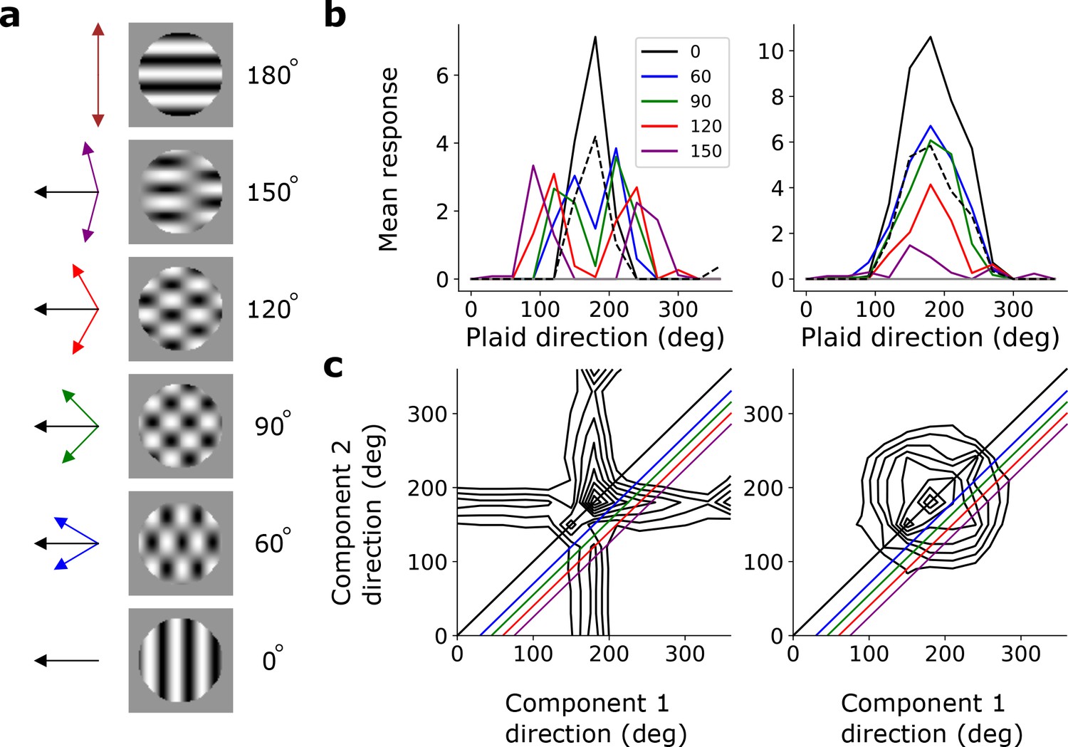
Pattern sensitivity.

(a) Example plaid stimuli used to measure pattern selectivity. Black arrow, direction of pattern motion. Colored arrows, directions of component motion. (b) Direction tuning curves showing the response of an example component-motion-selective (left, from stack 2) and pattern-motion-selective (right, from stack 4) unit to grating and plaid stimuli. Colored lines, response to plaid stimuli composed of gratings with the indicated angle between them. Black solid line, unit’s response to double intensity grating moving in the same direction as plaids. Black dashed line, response to single intensity grating moving in the same direction. Horizontal gray line, response to blank stimulus. (c) Surface contour plots showing response of units in b to plaids as a function of the direction of the grating components. Colored lines denote loci of plaids whose responses are shown in the same colors in b. Contour lines range from 20% of the maximum response to the maximum in steps of 10%. For clarity, all direction tuning curves are rotated so that the preferred direction of the response to the optimal grating is at 180°. Responses are mean amplitudes over time.

Figure 9

Download asset Open asset

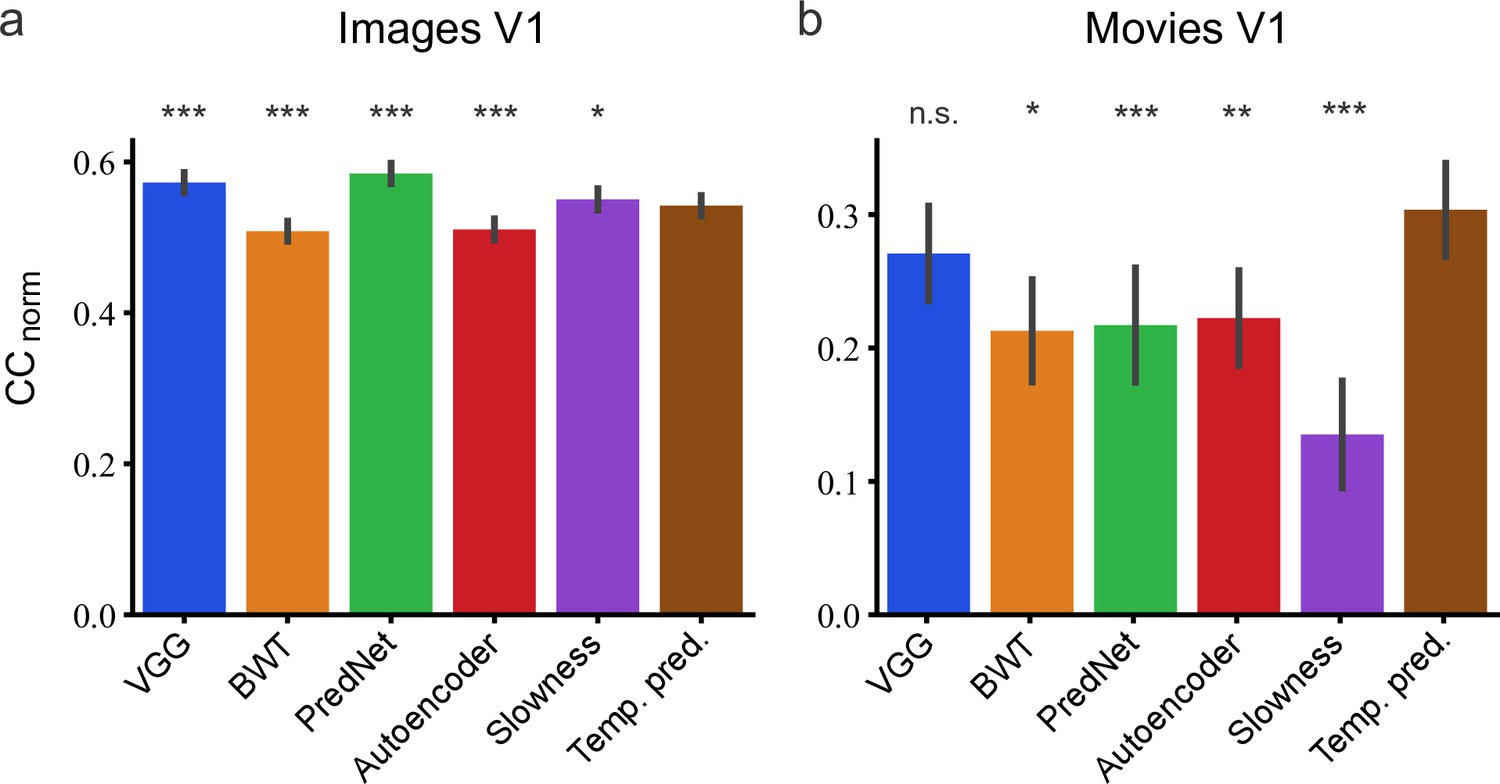
Assessment of different models in their capacity to predict neural responses in macaque V1 to natural stimuli.

(a) Prediction performance for neural responses to images (n = 166 neurons). Neural data from Cadena et al., 2019. (b) *Prediction performance for neural responses to movies (n* = 23 neurons). Neural data from Nauhaus and Ringach, 2007 and Ringach and Nauhaus, 2009. The error bars are standard errors for the population of recorded neurons. Prediction performance that does not differ significantly by a bootstrap method (see Methods) from the temporal prediction model is marked by n.s., while significantly different CC_norm values are denoted by *p <0.05, **p <0.01, ***p <0.001.

Tables

Table 1

Model parameter settings for each stack.

Stack	Input size (X,Y,T,I)	Hidden layer size	Kernel size (X’,Y’,T’)	Spatial and temporal extent	Stride (s₁,s₂,s₃)	Number of convolutional hidden units	Learning rate (α)	L₁ regularization strength (λ)
1	181x18x20x1	17x17x16x50	21x21x5	21x21x5	10,10,1	50	10^–2	10^-4.5
2	17x17x16x50	15x15x12x100	3x3x5	41x41x9	1,1,1	100	10^–4	10^–6
3	15x15x12x100	13x13x8x200	3x3x5	61x61x13	1,1,1	200	10^–4	10^–6
4	13x13x8x200	11x11x4x400	3x3x5	81x81x17	1,1,1	400	10^–4	10^–6

Additional files

Transparent reporting form: https://cdn.elifesciences.org/articles/52599/elife-52599-transrepform1-v2.docx
Download elife-52599-transrepform1-v2.docx

Download links

A two-part list of links to download the article, or parts of the article, in various formats.

Downloads (link to download the article as PDF)

Open citations (links to open the citations from this article in various online reference manager services)

Mendeley

Cite this article (links to download the citations from this article in formats compatible with various reference manager tools)

Yosef Singer
Luke Taylor
Ben DB Willmore
Andrew J King
Nicol S Harper

(2023)

Hierarchical temporal prediction captures motion processing along the visual pathway

eLife 12:e52599.

https://doi.org/10.7554/eLife.52599

Share this article

Cite this article

An illustration of the general architecture of the hierarchical temporal prediction model.

Architecture and operations performed by temporal prediction, predictive coding and PredNet models.

Hierarchical temporal prediction model in detail, with convolution.

RFs of trained first stack of the model show retina-like tuning.

Qualitative tuning properties of example model units in stack 2.

Tuning properties of example units in stack 2.

Qualitative tuning properties of example model units in stack 3.

Tuning properties of example units in stack 3.

Tuning properties of example units in stack 4.

Quantitative tuning properties of model units in stacks 2–4 in response to drifting sinusoidal gratings and corresponding measures of macaque V1 neurons.

Linear RFs of model units that could be well fitted by Gabors and corresponding Gabors.

Linear RFs of model units that could not be well fitted by Gabors and corresponding Gabors.

Linear RFs of model units and corresponding Gabors for stacked autoencoding (present-predicting) model.

Quantitative tuning properties of stacked autoencoding (present-predicting) model units in stacks 2–4 in response to drifting sinusoidal gratings and corresponding measures of macaque V1 neurons.

Linear RFs of model units and corresponding Gabors for the model with the input weights to each unit in the network shuffled across space and time.

Quantitative tuning properties of the model with input weights to each unit shuffled across space and time for units in stacks 2–4 in response to drifting sinusoidal gratings and corresponding measures of macaque V1 neurons.

Progression of tuning properties across stacks of the hierarchical temporal prediction model.

Pattern sensitivity.

Assessment of different models in their capacity to predict neural responses in macaque V1 to natural stimuli.

Model parameter settings for each stack.

Transparent reporting form

Downloads (link to download the article as PDF)

Open citations (links to open the citations from this article in various online reference manager services)

Cite this article (links to download the citations from this article in formats compatible with various reference manager tools)