Nuclei determine the spatial origin of mitotic waves
- Laboratory of Dynamics in Biological Systems, Department of Cellular and Molecular Medicine, Faculty of Medicine, KU Leuven, Belgium
- MeBioS - Biosensors Group, Department of Biosystems, KU Leuven, Belgium
- Department of Pharmaceutical Chemistry, United States
Figures
Box 1—figure 1
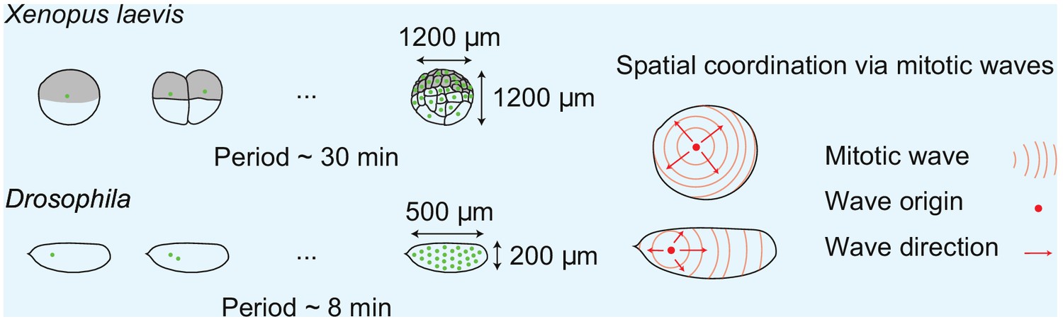
Spatial cell cycle coordination in early frog and fly embryos.
Box 2—figure 1

Reconstituting cell cycle oscillations using cell-free extracts.
Figure 1 with 6 supplements
Nuclei serve as pacemakers to organize mitotic waves.
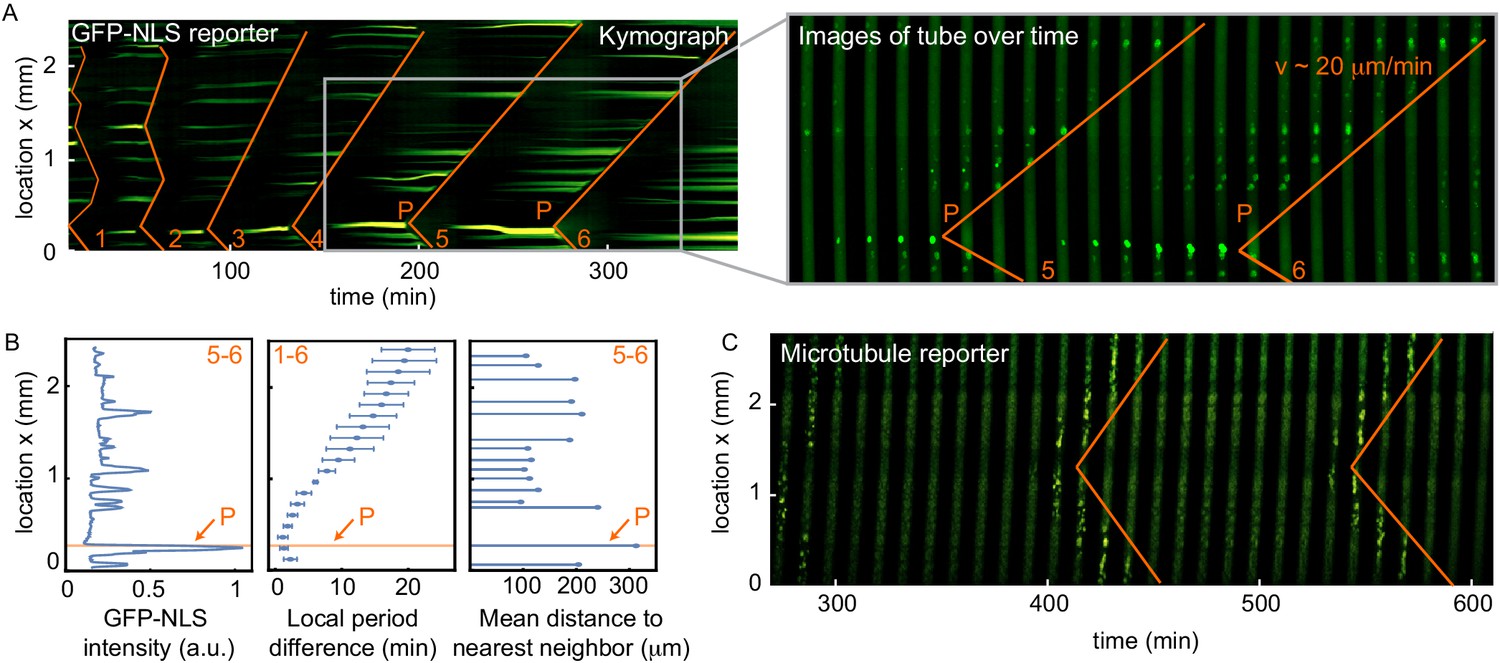
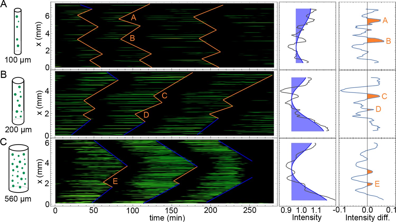
(A) Mitotic waves (orange) in a kymograph of cell-free extract experiment in a 100 µm Teflon tube. Wave dynamics are shown for cell cycle 1–6. For each time point we reduced the data from two to one spatial dimension by plotting the maximal GFP-NLS intensity along the transverse section of the tube. In the zoom, indicated by the gray box, we show snapshots of the whole 100 µm wide tube for different time points. The pacemaker location in cell cycle six is indicated by P. Approx. 250 nuclei/µl are added. (B) Analysis for the experiment in A. Left: GFP-NLS intensity profile, averaged over the times between the mitotic waves in cell cycle 5 and 6. The GFP-NLS intensity is highest close to the pacemaker region P. Middle: Difference in cell cycle period (with respect to the fastest period) at different locations along the tube, averaged over cell cycle 1–6, showing that the pacemaker region oscillates fastest. Right: Mean distance from the center of each nucleus to its two nearest neighboring nuclei. The nucleus close to the pacemaker region P is most separated from its neighbors. (C) Mitotic waves in a 200 µm Teflon tube shown by a fluorescent microtubule reporter (HiLyte Fluor 488).
Figure 1—figure supplement 1
Methodology of image analysis of the experiments.
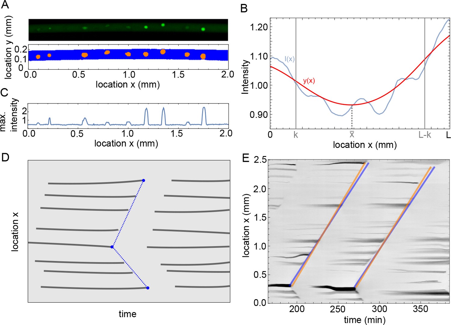
(A) Example of microscope image (top) and binarized image from ilastik (bottom), with in blue pixels recognized as background and orange the nuclei. (B) Intensity profile in blue and the filtered profile in red. The domain width is equal to and the parameter determines the boundary domain. (C) Maximum intensity over as function of , calculated for the microscope image in A. (D) Sketch of analysis of mitotic waves in a kymograph. At every time a profile is calculated as in C, when this is plotted over time the appearance and disappearance of nuclei is visible. The disappearance of nuclei is manually detected by visual inspection, as indictated by the blue points. Our program then automatically draws lines between these points, representing the mitotic waves, and calculates periods and wave speeds. (E) Example of the methodology sketched out in panel D for actual data, showing two (parts of) mitotic waves. The orange and blue lines illustrate errors that could be made visually, but they lead to relatively small differences in estimated period and wave speed (up to 1 min difference in estimated period and up to 2 µm/min difference in estimated wave speed).
Figure 1—figure supplement 2

Analysis of the experiment in panel A, quantifying the time evolution of the number of nuclei, the nuclear size, the internuclear distance, the oscillation period, the intensity of the nuclei, and the observed wave speed.
Analysis of the experiment shown in Figure 1. We plotted as function of the cycle number: the number of nuclei (A), the nuclear size (B), the observed wave speed (C), the period of the oscillation (D), the intensity of the nuclei (E), and the internuclear distance (F). Blue is individual data, orange lines give the median and the orange area is the 2/3 -interval. Red dots in (E) highlight the nuclei that are pacemakers. The internuclear distance is further analyzed in panels G and H, showing the averaged autocorrelation of projected binarized images (G) and a histogram of the distances between nuclei for all binarized images (H). Both analyses of the nuclear distribution show that the distance between neighboring nuclei is typically around 150 µm. (I) shows the same analysis as in (H), but now for an experiment in a 100 µm Teflon tube for ≈ 60 added sperm nuclei/µl.
Figure 1—figure supplement 3
Analysis of the spatial GFP-NLS intensity profile and the internuclear distances for multiple experiments.
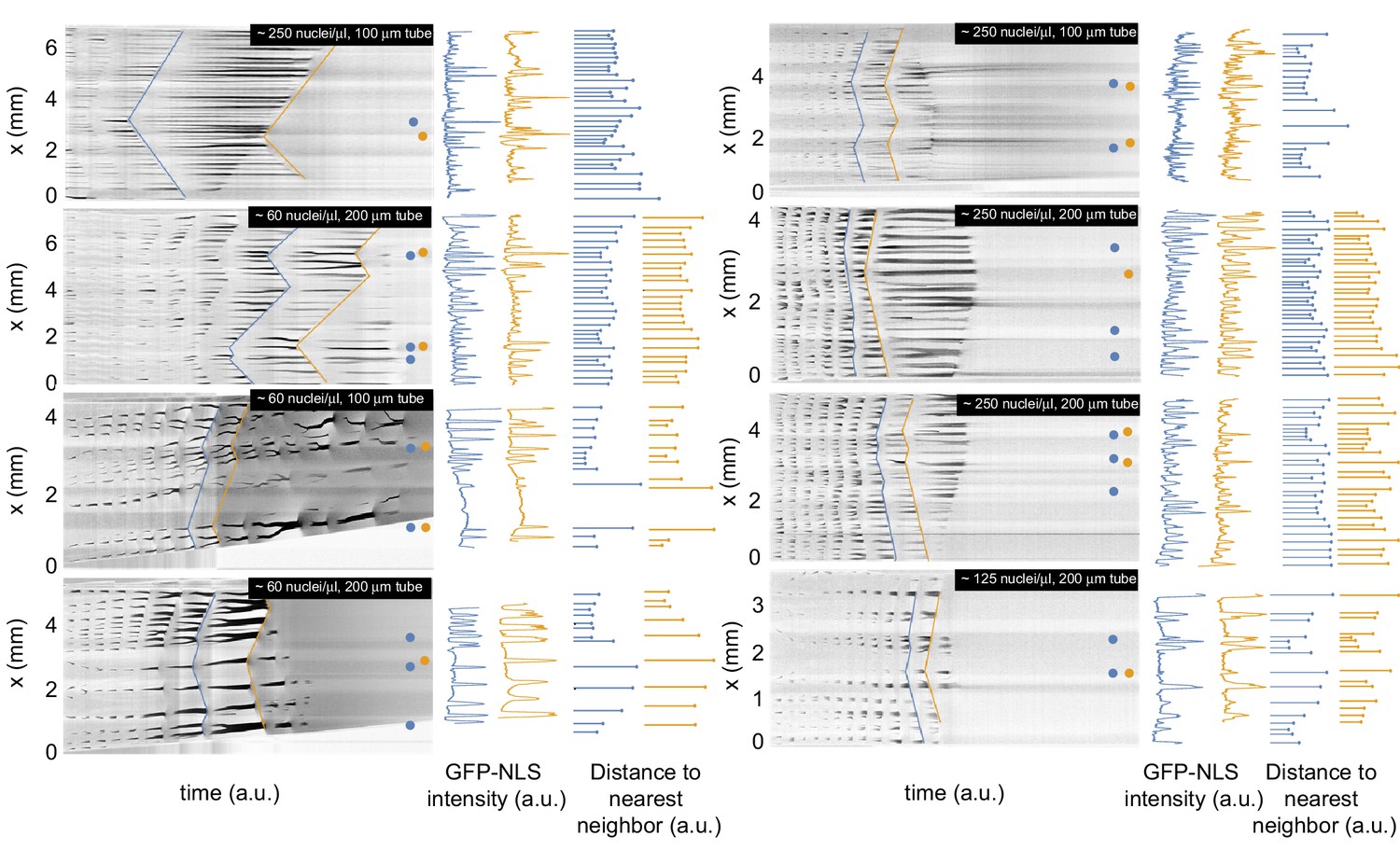
Kymographs of the GFP-NLS intensity for eight additional experiments in tubes of 100 and 200 µm, with a corresponding analysis of the spatial GFP-NLS intensity profile and the internuclear distances. The dots on the kymographs indicate the location of the pacemakers for two consecutive cell cycles indicated in blue and orange.
Figure 1—figure supplement 4
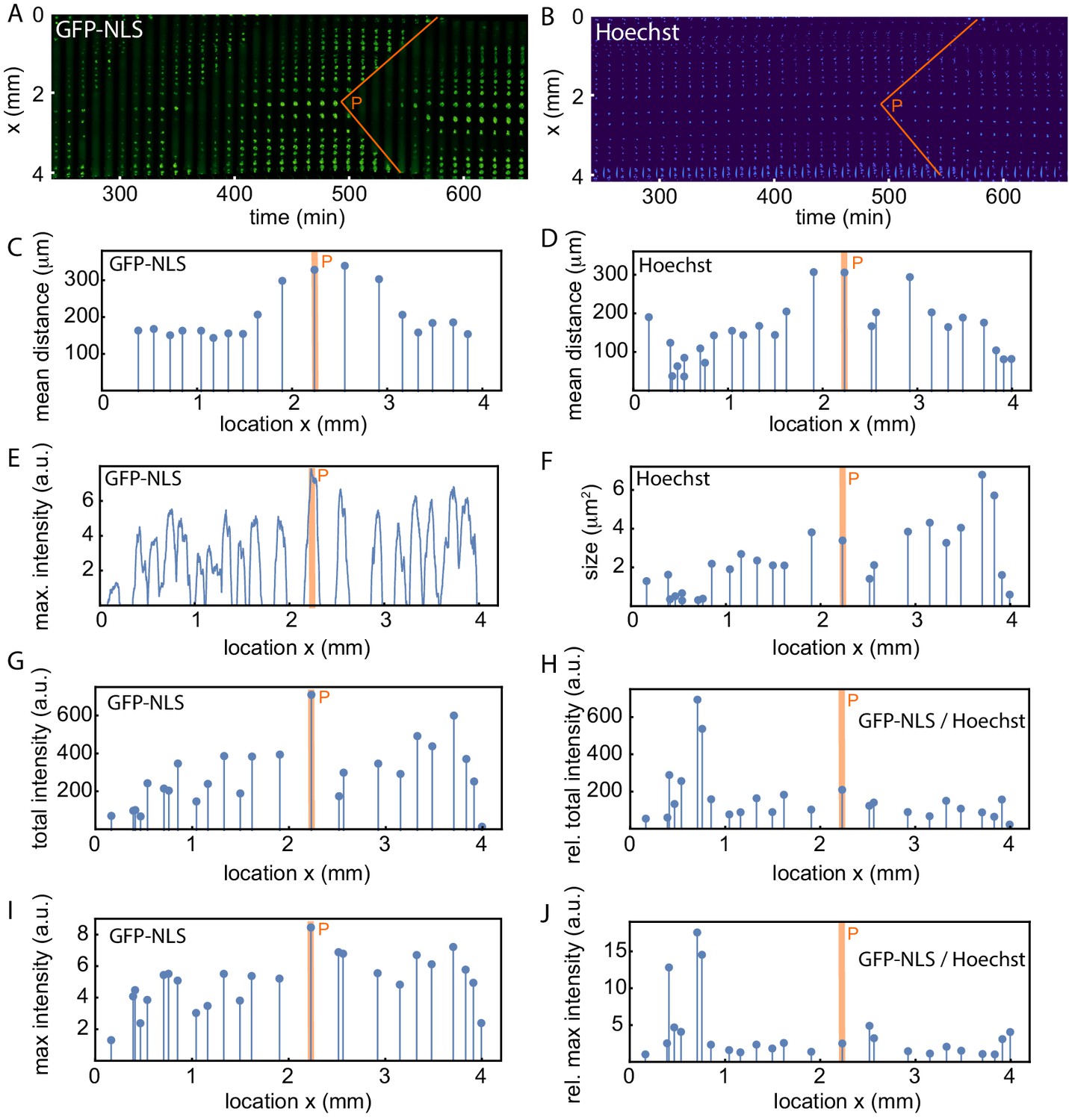
Analysis of the spatial GFP-NLS and Hoechst intensity profile and the internuclear distances.
(A) Mitotic waves (orange) in a kymograph of cell-free extract experiment in a 200 µm Teflon tube, using the GFP-NLS reporter. (B) Same as A, but using DNA staining (Hoechst 33342). C-J show an analysis of the experiment in A-B. (C,D) Mean distance from the center of each nucleus to its two nearest neighboring nuclei using the GFP-NLS and the Hoechst signal, respectively. (E) GFP-NLS intensity profile, averaged over the times between two mitotic waves. (F) Nuclear size in a single cell cycle determined from the Hoechst signal. G. Total GFP-NLS intensity per nucleus in a single cell cycle. (I) Maximal GFP-NLS intensity per nucleus in a single cell cycle. (H, J) Total and maximal GFP-NLS intensity per nucleus normalized by the nuclear size in a single cell cycle.
Figure 1—video 1
Video of the cell-free extract experiment in panel A, B.
8.86 hr of experiment in 484 frames, scale bar is 200 µm.
Figure 1—video 2
Video of the cell-free extract experiment in panel C.
15.68 hr of experiment in 79 frames, scale bar is 200 µm.
Figure 2 with 4 supplements
Nuclear density and nuclear import strength control cell cycle period and mitotic wave speed.
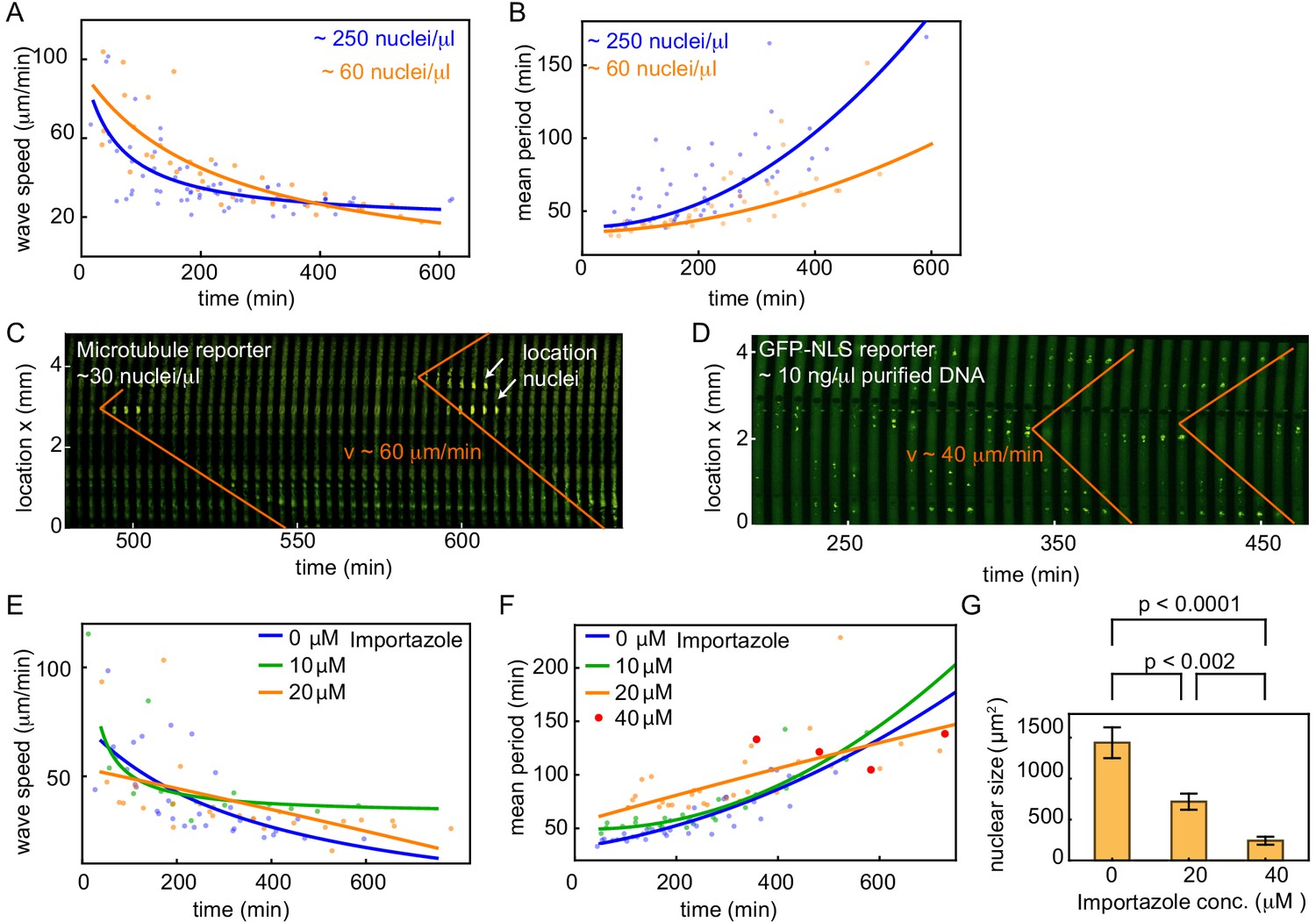
(A,B) Wave speed (A) and cell cycle period (B) over time obtained for N = 19 analyzed 100 and 200 µm Teflon tube experiments using the GFP-NLS reporter. Results are pooled from 11 different cell-free extracts for two different nuclear concentrations: ≈ 60, and ≈ 250 nuclei/µl. Each plotted point corresponds to the minimal wave speed or average cell cycle period in a single cell cycle of a single tube experiment. (C) Mitotic waves in a 200 µm Teflon tube using a GFP-MT reporter with few nuclei (≈ 30 nuclei/µl). Nuclear locations are identified in bright-field and indicated here. (D) Mitotic waves in a 200 µm Teflon tube using a GFP-NLS reporter with ≈ 10 ng/µl of added purified DNA. (E,F) Wave speed (E) and cell cycle period (F) over time obtained for N = 16 analyzed 200 µm Teflon tube experiments using the GFP-NLS reporter. Results are pooled from two different cell-free extracts for four different concentrations of the nuclear import inhibitor importazole: 0, 10, 20, 40 µM. Nuclear concentration: ≈ 250 nuclei/µl. Each plotted point corresponds to the minimal wave speed or average cell cycle period in a single cell cycle of a single tube experiment. (G) Mean nuclear size in the presence of varying concentrations of the nuclear import inhibitor importazole: 0, 20, 40 µM. Two tube experiments were analyzed per condition, which gave us nuclear sizes for 75, 62, and 25 nuclei, for 0, 20, 40 µM importazole, respectively. Error bars are one standard deviation of the mean.
Figure 2—figure supplement 1
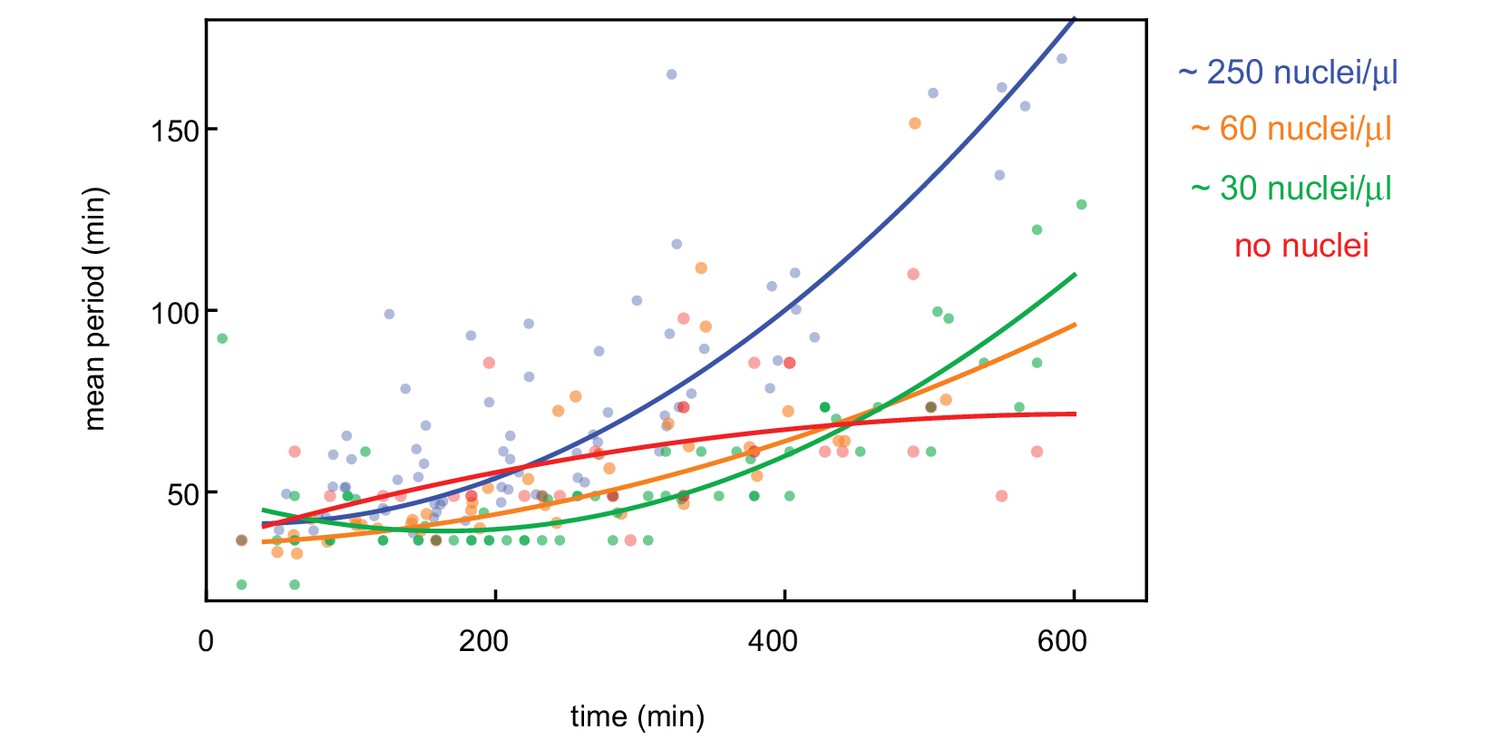
Influence of nuclear density on cell cycle period.
Cell cycle period over time obtained for N = 27 analyzed 100 and 200 µm Teflon tube experiments using the GFP-NLS reporter. Results are pooled from 14 different cell-free extracts for four different nuclear concentrations: 0, ≈ 30, ≈ 60, and ≈ 250 nuclei/µl. Each plotted point corresponds to the minimal wave speed or average cell cycle period in a single cell cycle of a single tube experiment. Note that for 0, ≈ 30 nuclei/µl, cell cycle periods could not be calculated as explained in the Image Analysis section due to the lack of nuclei with a GFP-NLS signal. Instead, they have been determined manually by looking at periodic variations in the microtubule reporter at different locations in the tube.
Figure 2—figure supplement 2
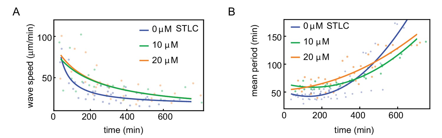
Influence of Eg5 kinesin inhibitor on wave speed and cell cycle period.
Wave speed (A) and cell cycle period (B) over time obtained for N = 17 analyzed 200 µm Teflon tube experiments using the GFP-NLS reporter. Results are pooled from three different cell-free extracts for three different concentrations of the Eg5 kinesin inhibitor STLC: 0, 10, 20 µM. Nuclear concentration: ≈ 250 nuclei/µl. Each plotted point corresponds to the minimal wave speed or average cell cycle period in a single cell cycle of a single tube experiment. .
Figure 2—video 1
Video of the cell-free extract experiment in panel D.
Mitotic waves in a 200 µm wide Teflon tube using a GFP-NLS reporter with ≈ 10 ng/µl of added purified DNA. 14.96 hr of experiment in 94 frames, scale bar is 200 µm.
Figure 2—video 2
Video of the cell-free extract experiment in panels E-G.
Mitotic waves in a 200 µm wide Teflon tube using a GFP-NLS reporter with 40 µM nuclear import inhibitor importazole. Nuclear concentration: ≈ 250 nuclei/µl. 19.49 hr of experiment in 189 frames, scale bar is 200 µm.
Figure 3 with 6 supplements
A model where nuclei spatially redistribute cell cycle regulators predicts the location of pacemaker regions.
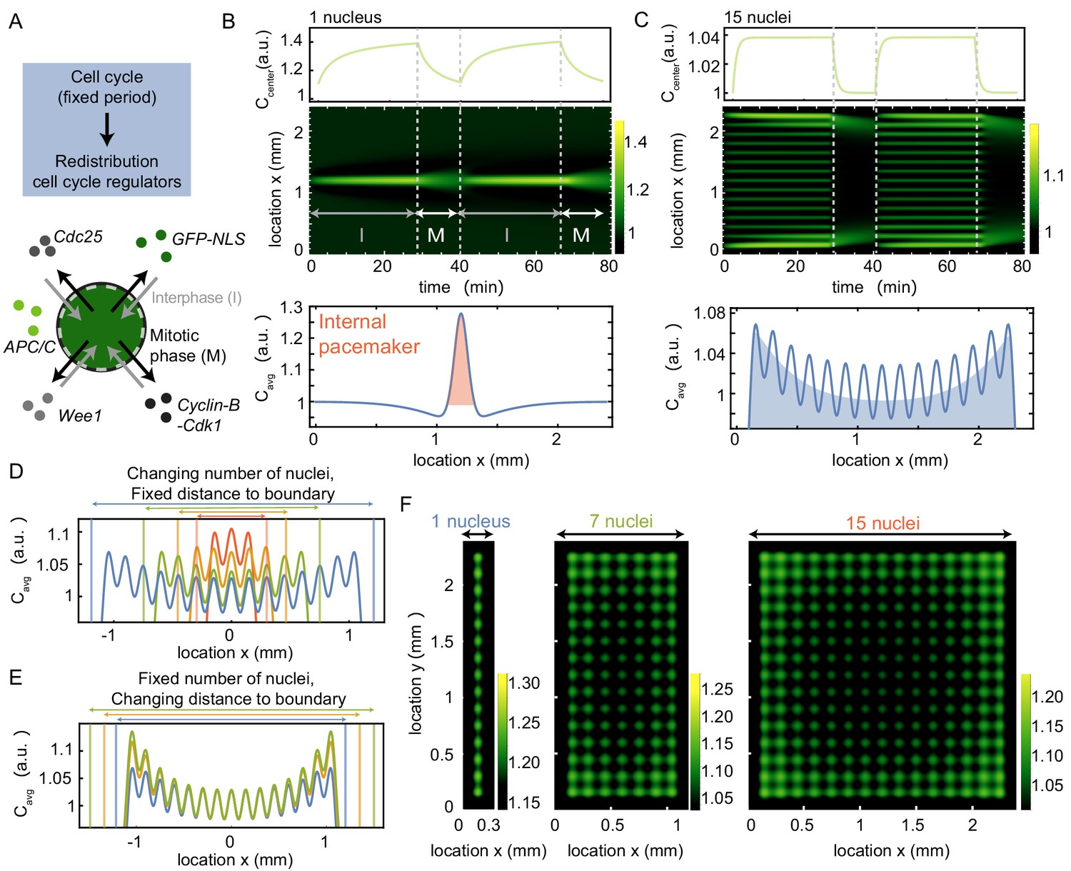
(A) Schematic of the two phases of the model, interphase (import of regulators) and mitotic phase (diffusion). The cell cycle has a fixed period, which controls the periodic spatial redistribution of regulators. (B) Time evolution of Equation (8) in Appendix 1 in one spatial dimension for one nucleus, with the concentration C at the center of the domain shown in the top panel. The profile below is the time average of the intensity over one cell cycle period (), where the red area highlights the build-up of cell cycle regulators close to the nucleus. The intensity is normalized such that . Parameters: µm3/min, µm, , min, µm2/min and constant initial condition . Domain size is 2400 µm. (C) Same as B, but now for 15 nuclei, where the time-averaged profile shows an overall build-up of regulators towards the boundary (see blue shaded area). (D) Same as C, but now varying the number of nuclei in the system, while keeping the distance of the outer nucleus to the system boundary constant. The total system size changes as a result of the changing number of nuclei. (E) Same as C, but now varying distances of the outer nucleus to the system boundary (), while keeping the number of nuclei constant. The total system size changes as a result of the changing distance to the boundary . (F) Same as B and C, but in a rectangular system of two spatial dimensions. The length of the system is fixed to 2400 µm, while the width of the system increases from 300 µm (with one nucleus) to 2400 µm (with 15 nuclei). The time-averaged profile is plotted, again illustrating the overall build-up of regulators towards the boundary.
Figure 3—figure supplement 1
Influence of the distance of the outer nuclei to the system boundary on the build-up of regulators at the boundary.
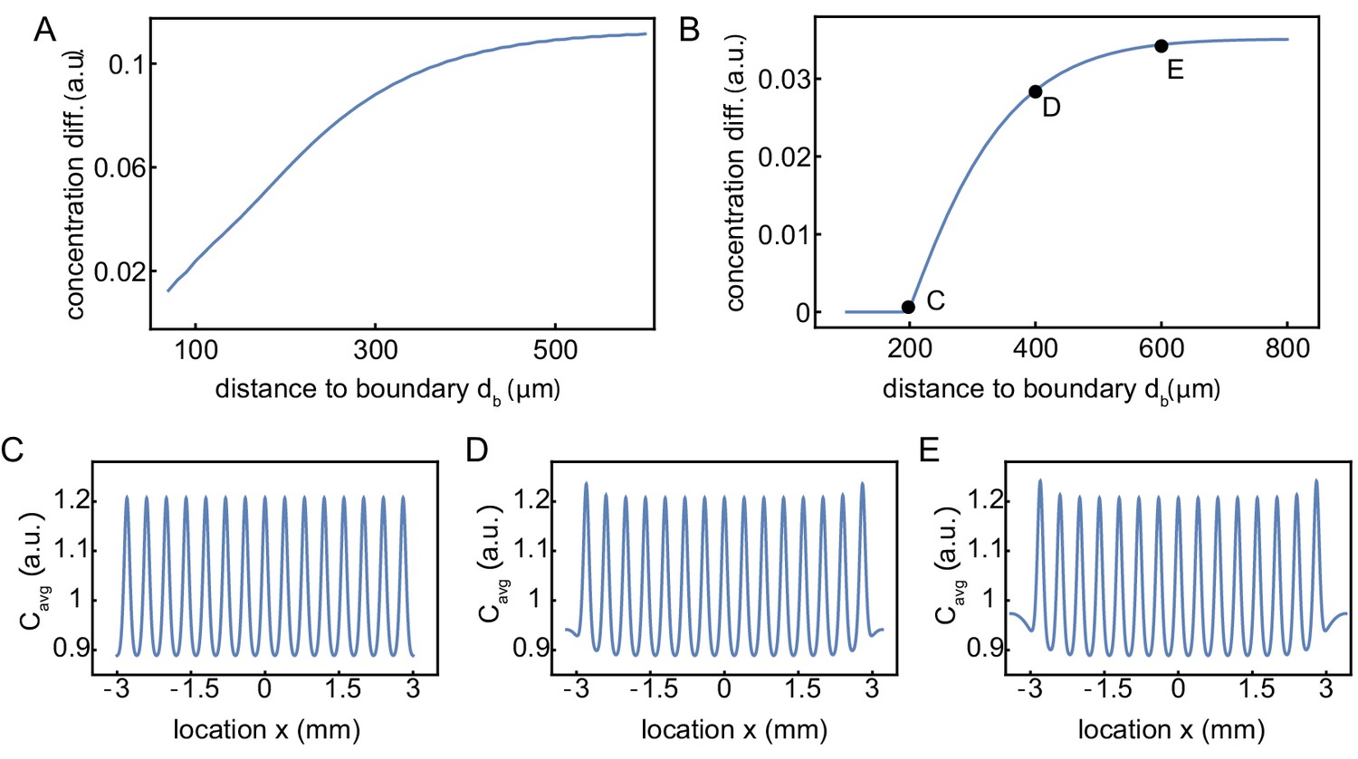
Influence of the distance of outer nuclei to the system boundary on the build-up of regulators at the boundary. (A) Same simulations as in Figure 3E, but continuously varying the distance of the outer nuclei to the system boundary. The strength of the build-up of regulators at the boundary is found to saturate as increases. This boundary strength is defined as the relative difference of the maximum (at the boundary) with respect to the background value in the middle, of the intensity profile averaged over time. The internuclear distance is 150 µm. (B) Same as A, but now for 15 nuclei with an increased internuclear distance of 400 µm. The distance of the outer nuclei to the system boundary needs to be larger than 200 µm (half of the internuclear distance) to have a build-up of regulators at the boundary. (C-E) Examples of the concentration profiles at = 200, 400, 600, respectively. The internuclear distance is 400 µm.
Figure 3—figure supplement 2
Influence of system parameters on the build-up of regulators at the boundary.
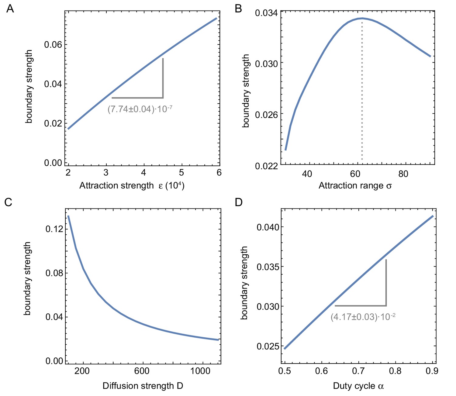
Influence of system parameters on the build-up of regulators at the boundary. We define the boundary strength as the relative difference of the maximum (at the boundary) with respect to the background value in the middle, of the intensity profile averaged over time. (A) The strength of the effect increases with the attraction strength (related to the nuclear import rate). (B) The boundary strength is found to be maximal for a certain attraction range . If is too small, the nuclei are too far apart to effectively compete for shared resources, leading to a small boundary strength. When is too large, however, the regions of attraction overlap so much that multiple nuclei are ‘competing’ for the same proteins, again leading to a smaller boundary strength. Interestingly, the optimal attraction range ≈ 150m ( corresponding to ) corresponds to the size of the nuclear domain reported in Landing et al., 1974; Telley et al., 2012 and the experimentally measured internuclear distance (Figure 1—figure supplement 2G–I, Figure 3—figure supplement 5). (C) The build-up of protein regulators at the boundary also decreases with increasing diffusion strength, effectively washing out the effect during mitosis. (D) Similarly, the boundary effect is thus also more pronounced with increasing , as this decreases the mitotic phase during which regulators are free to diffuse. Parameters (if not otherwise specified): .
Figure 3—figure supplement 3
Influence of deviations to a perfect nuclear pattern in 1D on the build-up of regulators at the boundary.
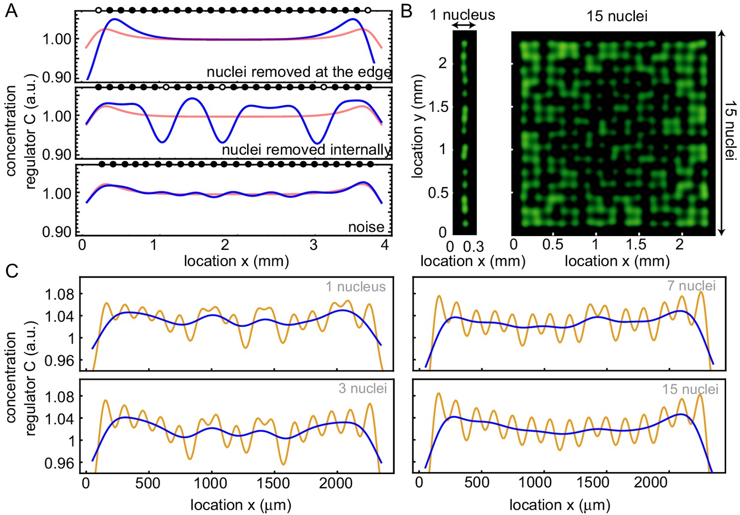
(A) Different nuclear positioning influences the concentration profile (blue). The average concentration profile of the control is shown in red for comparison. The black dots denote the positions of the nuclei, while they are white when nuclei are absent. Top: deleted nuclei at the boundary (1 and 25), middle: deleted three nuclei randomly, bottom: adding noise to nuclei positions. (B) Repetition of the simulations in Figure 3D with noise on the positions of the nuclei, for one row (left) and 15 rows (right) of nuclei in the x direction. (C) Averaged projection on the y direction (orange) and the filtered signal (blue) of that profile, for 1, 3, 7 and 15 rows of nuclei (similar as in Figure 3D,E) with noise on the nuclear positions.
Figure 3—figure supplement 4
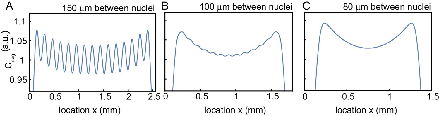
Influence of internuclear distance on the build-up of regulators at the boundary.
Influence of internuclear distance on the build-up of regulators at the boundary. Same simulations as in Figure 3C, but changing the internuclear distance from 150 µm (A) to 100 µm (B) to 80 µm. The number of nuclei is kept fixed to 15 nuclei.
Figure 3—figure supplement 5
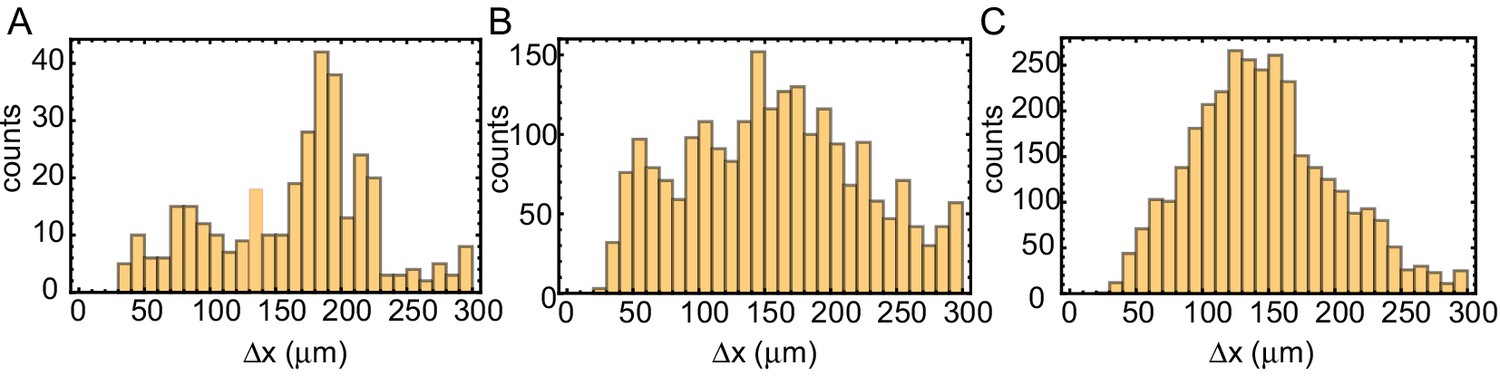
Internuclear distance in tubes of varying width.
Distance analysis of the tube experiments shown in Video 2 of the paper. Tube widths are 100 µm (A), 200 µm (B) and 560 µm (C). From the binarized kymographs, the centers of the nuclei are detected. For all nuclei, the (center-center) distances to the two nearest neighbors are calculated and after subtracting doubly counted distances shown in these histograms.
Figure 3—figure supplement 6

Influence of varying system widths in 2D on the build-up of regulators at the boundary.
Strength of the build-up of regulators at the boundary in 2D with increasing system width and number of rows of nuclei. This boundary strength is defined as the relative difference of the maximum (at the boundary) with respect to the background value in the middle, of the intensity profile averaged over time.
Figure 4 with 2 supplements
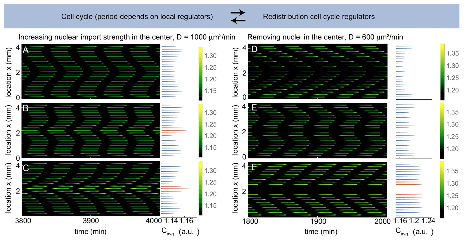
Multiple pacemakers compete to define the direction of mitotic waves.
Time evolution of Equation (21) in Appendix 1 in one spatial dimension. The profile on the right is the time average of the intensity over one cell cycle period (). The intensity is normalized such that . Parameters: µm3/min, µm, and initial condition . (A-C) µm2/min, domain size is 4400 µm including 21 nuclei separated by 200 µm. is defined as a factor by which the nuclear import strength is increased in the middle nucleus (see Appendix 1). is 1 (A), 1.04 (B) and 1.08 (C). Upon increasing the nuclear import strength of the middle nucleus, a transition is observed from boundary-driven waves (A) to waves coming from an internal pacemaker (C). The internal pacemaker region has a higher average concentration of the regulator , as indicated in orange. For intermediate values of both types of waves coexist (B). (D-E) µm2/min, , domain size is 4400 µm. When 21 nuclei are regularly separated by 200 µm, a boundary-driven wave is observed (D). While removing the middle nucleus leads to the coexistence of boundary-driven waves and a waves coming from an internal pacemaker region close to the introduced gap (E), removing three of the middle nuclei abolishes the boundary-driven wave and only the wave coming from the internal pacemaker region persists.
Figure 4—figure supplement 1
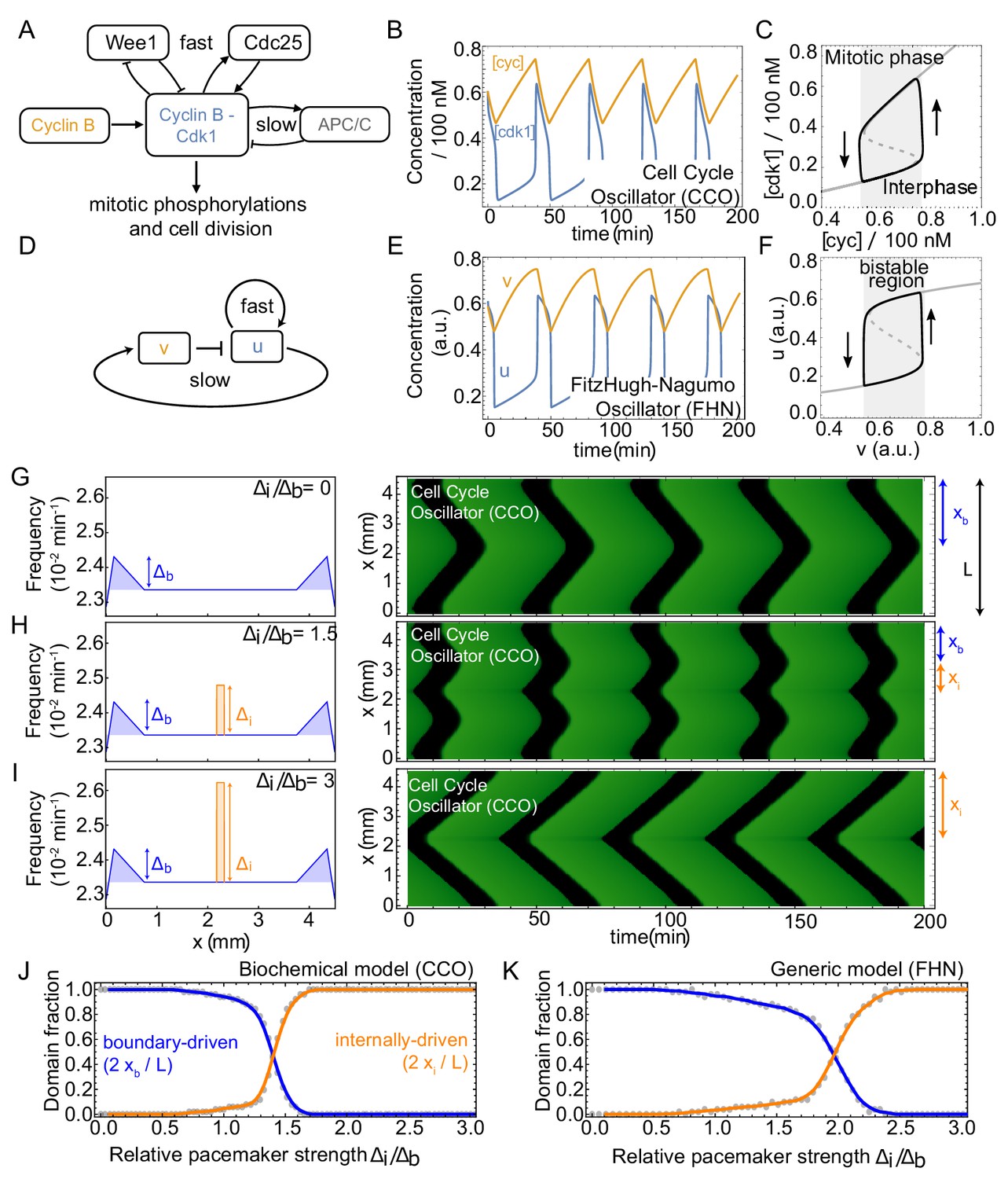
Competing pacemakers in known PDE models for cell cycle oscillations reproduce similar mitotic wave dynamics.
(A-F) show that models of different complexity are able to capture cell cycle oscillations. (A,D) Core components and interactions of the cell cycle oscillator model (CCO) and the FitzHugh-Nagumo oscillator model (FHN), respectively. (B,E) Time series of relaxation oscillations in the CCO and the FHN, respectively. CCO parameters are set on min-1, min-1, nM, and nM/min. For the biological meaning of the parameters, see Appendix 1. FHN parameters are set on and we applied the linear mapping such that the output of both CCO and FHN models are similar. C,F. Phase space projection of the time series of the limit cycle solutions corresponding to (B,E), including nullclines of resp. [cdk1] and . (G) Numerical simulation of the cell cycle oscillator (CCO) model where the Cdc25-related parameters ( and ) are changed in space to define a spatially heterogeneous frequency profile. The left panel shows that the frequency is increased by at the boundary with respect to the cell cycle frequency elsewhere in the domain (see blue shaded region). The right panel illustrates the time series after a transient of ∼ 80 cycles in a domain of size mm. Boundary-driven waves are found to coordinate the whole domain (). (H) Same as A, but now a second internal pacemaker region is introduced (frequency increased by as indicated by orange region). Waves originating at the boundary and at the internal pacemaker region coexist (). (I) Same as B, but with . Mitotic waves are now dominated by the internal pacemaker (). (J) Domain fractions controlled by waves starting from the boundary () and from the internal pacemaker (). is kept constant, while is changed for each simulation using the CCO model. K. Same as J, but for the FitzHugh-Nagumo (FHN) model.
Figure 4—figure supplement 2
Boundary-driven waves can exist in spatially-extended systems based on different types of oscillators.
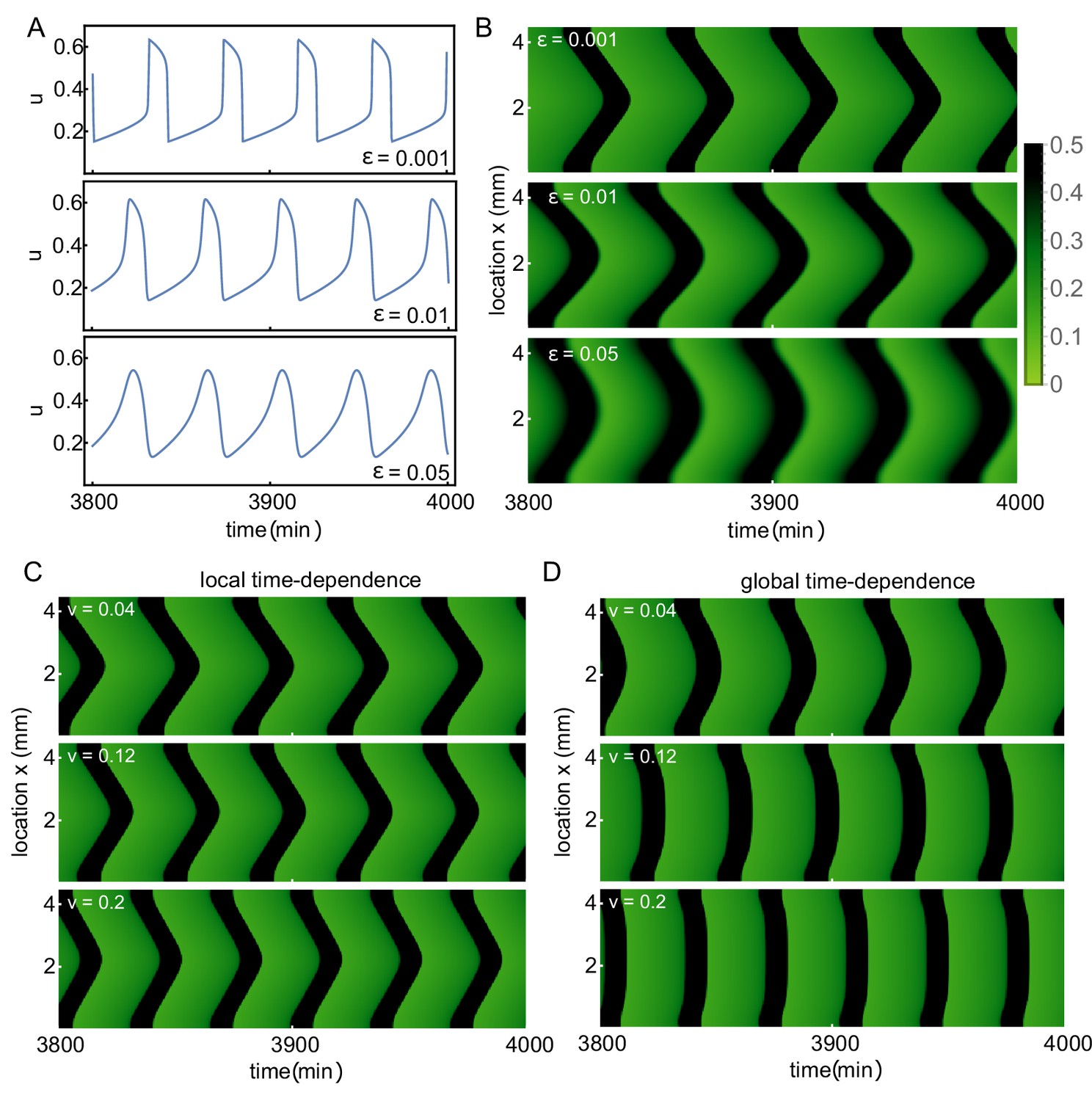
Boundary-driven waves can exist in spatially-extended systems based on different types of oscillators. We study the dynamics of mitotic waves using the same numerical setup as in Figure 4—figure supplement 1. (A) Time traces for the FitzHugh-Nagumo (FHN) model are shown for changing values of , a measure for the timescale separation in the system. When increasing oscillations become more sinusoidal and less relaxation-like. (B) Kymographs, corresponding to the oscillations shown in A, show that boundary-driven waves persist when varying . (C,D) The effect of using time-dependent parameters in the FHN system on the existence and properties of boundary-driven waves. Parameters are changed with different velocities, either locally (C) or globally (D) (for more details, see Appendix 2). The kymographs are shown for three different velocities. Whereas boundary-driven waves persist, their wave speed increases with this velocity. In the global case (D), mitotic waves in the presence of such time-dependent changes have been dubbed 'sweep waves’ (Vergassola et al., 2018).
Figure 5 with 5 supplements
Wider systems lead to boundary-driven mitotic waves.
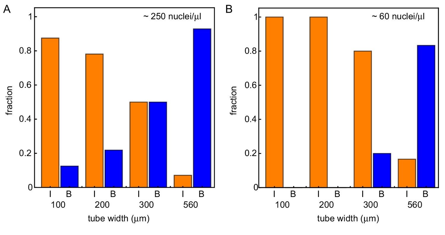
Fraction of experiments dominated by internally-driven waves (‘I’) and by boundary driven waves (‘B’), evaluated at the end of each of the imaged tubes of varying width and varying concentration of demembranated sperm nuclei. Cases where both wave types coexist (‘IB’) are counted half in each category. This is done for two different concentration of demembranated sperm nuclei: ≈ 250 nuclei/µL extract (A) or ≈ 60 nuclei/µL extract (B). For panel A (B), results are obtained for N = 49 (17) analyzed Teflon tube experiments using the GFP-NLS reporter, and they are pooled from 23 (7) different cell-free extracts.
Figure 5—figure supplement 1
Kymographs of mitotic waves in tubes of varying width.
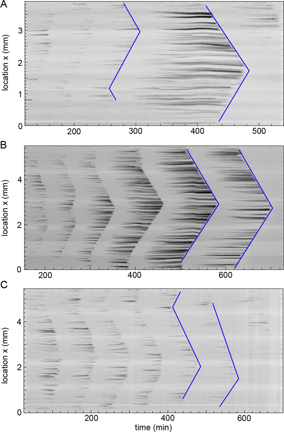
Kymographs corresponding to the experiments shown in Video 2 for the tubes of 100 µm (A), 200 µm (B), and 560 µm (C) in diameter. Boundary-driven waves are indicated by blue lines, while mitotic waves driven by internal pacemakers are highlighted by orange lines. On the right hand side, the corresponding averaged GFP-NLS intensity profiles are shown in black. Slow spatial changes are highlighted in blue. The resulting profiles after removing these slower changes are then shown in orange, highlighting internal pacemakers regions with a higher GFP-NLS intensity (A–E). Approx. 250 nuclei/µl are added.
Figure 5—figure supplement 2
Kymographs of mitotic waves in thick tubes (560 µm diameter).
Three representative experiments in the thickest tubes with a diameter of 560 µm (corresponding to the situation in Figure 5—figure supplement 1C). Kymographs of mitotic waves (see blue lines) are shown which all converge to boundary-driven waves. Approx. 250 nuclei/µl are added.
Figure 5—figure supplement 3
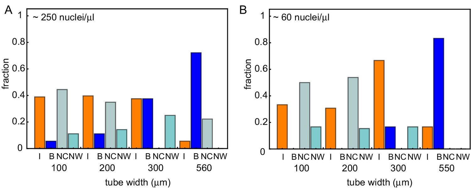
Analysis of all experiments, including those that did not cycle or did not show any wave dynamics.
We carried out 120 experiments in total, 89 with a concentration of ∼ 250 nuclei/µL extract and 31 with a concentration of ∼ 60 nuclei/µL extract. These data also included experiments that showed few cell cycle oscillations, where we discarded all experiments that cycled less than five times (labeled as NC - No Cycling). We also discarded experiments which did not show clear mitotic wave behavior (labeled as NW - No Waves). For all experiments that showed wave behavior and has sufficient cycles, we then characterized its behavior towards the end of the experiment in three ways: (i) waves emerge from an internal pacemaker (labeled as I), (ii) waves emerge from the boundary (labeled as B), (iii) or waves emerge both internally and from the boundary (in which case we considered this experiment as 50% I and 50% B). All data including NC/NW for full tubes and concentrations of ∼ 250 nuclei/µL extract (left) and ∼ 60 nuclei/µL extract (right).
Figure 5—figure supplement 4
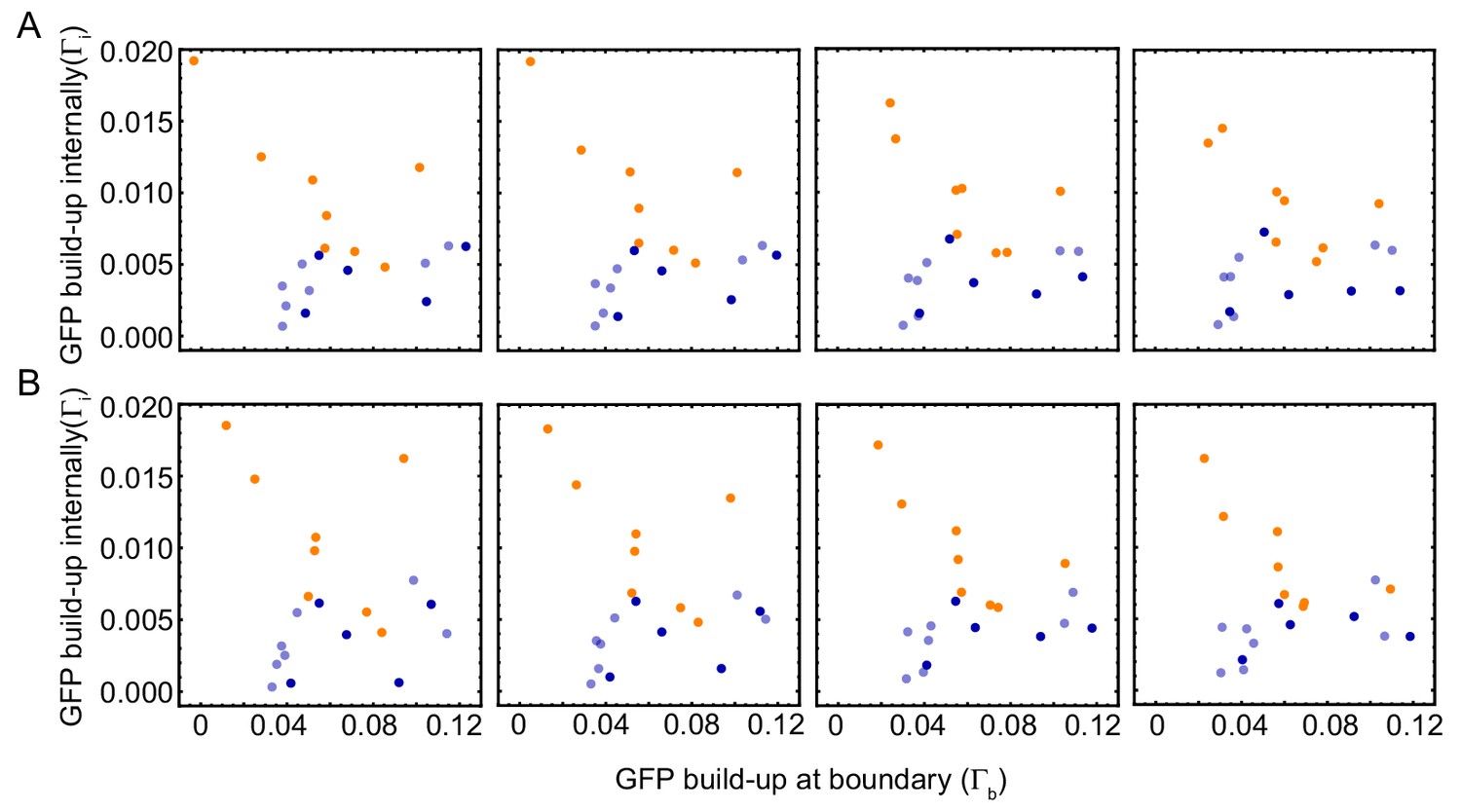
Robustness of image analysis of experiments.
GFP-NLS strength of internal peaks () vs. the GFP-NLS boundary strength () for , (A) and for , (B). Colors denote the type of observed mitotic waves: orange for boundary-driven waves, and blue for waves driven by internal pacemakers. Wave speed and cell cycle period for varying tube width. Wave speed (A,C) and cell cycle period (B,D) over time obtained for N = 27 analyzed Teflon tube experiments using the GFP-NLS reporter. Results are pooled from 15 different cell-free extracts for ≈ 250 nuclei/µl. Tube width is 100, 200, 300, and 560 µm.
Figure 5—figure supplement 5
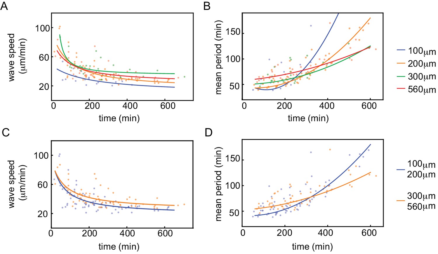
Wave speed and cell cycle period for varying tube width.
Wave speed (A,C) and cell cycle period (B,D) over time obtained for N=27 analyzed Teflon tube experiments using the GFP-NLS reporter. Results are pooled from 15 different cell-free extracts for ≈250 nuclei/µl. Tube width is 100, 200, 300, and 560 µm.
Videos
Video 1
Video of cell-free extract experiment in a 200 µm wide Teflon tube imaged in bright-field and using a fluorescent microtubule reporter (HiLyte Fluor 488). The experiment on the bottom (see also Figure 1C) has few nuclei (≈ 30 nuclei/µl), while no nuclei are added in the experiment on the top. In the presence of few nuclei, mitotic waves originate from those nuclei and propagate through the whole tube. In the absence of nuclei, no mitotic waves are observed to travel through the tube. Scale bar is 200 µm.
Video 2
Video of cell-free extract experiments in Teflon tubes of varying diameters (≈ 100, 200, 300 and 560 µm wide) and a thin droplet of ≈ 1 mm wide.
Imaging is done with the GFP-NLS reporter. Mitotic waves are found to originate from the boundary as the system becomes wider. Scale bar is 200 µm.
Tables
Key resources table
| Reagent type (species) or resource | Designation | Source or reference | Identifiers | Additional information |
|---|---|---|---|---|
| Strain, strain background (Xenopus laevis, male and female) | Xenopus laevis | Centre de Res- sources Biolo- giques Xénopes | RRID:XEP_Xla | |
| Recombinant DNA reagent | GFP-NLS | DOI: 10.1038/nature12321 | Construct provided by James Ferrell (Stanford Univ., USA) | |
| Peptide, recombinant protein | (fluorescent) microtubule reporter | Cytoskeleton, Inc | Cat. #: TL488M-B | |
| Commercial assay or kit | GenElute Mammalian Genomic DNA kit | Sigma-Aldrich | Cat. #: G1N70 | |
| Chemical compound, drug | Human chorionic gonadotropin | MSD Animal Health | CHORULON | |
| Chemical compound, drug | Pregnant mare’s serumgonadotropin | MSD Animal Health | FOLLIGON | |
| Chemical compound, drug | Calcium ionophore A23187 | Sigma-Aldrich | PubChem CID: 11957499; Cat. #: C7522 | |
| Chemical compound, drug | Leupeptin | Sigma-Aldrich | PubChem CID: 72429; Cat. #: L8511 | |
| Chemical compound, drug | Pepstatin | Sigma-Aldrich | PubChem CID: 5478883; Cat. #: P5318 | |
| Chemical compound, drug | Chymostatin | Sigma-Aldrich | PubChem CID: 443119; Cat. #: C7268 | |
| Chemical compound, drug | Cytochalasin B | Sigma-Aldrich | PubChem CID: 5311281; Cat. #: C6762 | |
| Chemical compound, drug | Proteinase K | Sigma-Aldrich | Cat. #: P2308 | |
| Chemical compound, drug | Importazole | Sigma-Aldrich | PubChem CID: 2949965; Cat. #: SML0341 | |
| Chemical compound, drug | S-Trityl-L-cysteine | Acros Organics | PubChem CID: 76044; Cat. #: 173010050 | |
| Software, algorithm | Fiji | http://fiji.sc/ | RRID:SCR_002285 | |
| Software, algorithm | Wolfram Mathematica | www.wolfram.com/mathematical | RRID:SCR_014448 | |
| Software, algorithm | Ilastik | www.ilastik.org | RRID:SCR_015246 | |
| Software, algorithm | Model for nuclear import | This paper, used for Figure 3 | Code on GitHub (Nolet, 2020) | |
| Software, algorithm | Model for nuclear import, frequency dependent | This paper, used for Figure 4 | Code on GitHub (Nolet, 2020) | |
| Other | Teflon tube | Cole-Parmer | Cat. #: 06417–11 | |
| Other | Hoechst 33342 | ImmunoChemistry technologies | RRID:AB_265113; Cat. #: 639 | (5 µg/mL) |
| Other | Leica TCS SPE confocal microscope | Leica Microsystems | RRID:SCR_002140 | |
| Other | Ultracentrifuge OPTIMA XPN - 90 | Beckman Coulter | RRID:SCR_018238; Cat. #: A94468 |
Additional files
Download links
A two-part list of links to download the article, or parts of the article, in various formats.
Downloads (link to download the article as PDF)
Open citations (links to open the citations from this article in various online reference manager services)
Cite this article (links to download the citations from this article in formats compatible with various reference manager tools)
Nuclei determine the spatial origin of mitotic waves
eLife 9:e52868.
https://doi.org/10.7554/eLife.52868


