A fully automated high-throughput workflow for 3D-based chemical screening in human midbrain organoids
- Department for Cell and Developmental Biology, Max Planck Institute for molecular Biomedicine, Germany
- Westfälische Wilhelms-Universität Münster, Germany
- Max Planck Research Group for RNA Biology, Max Planck Institute for molecular Biomedicine, Germany
- Research Group for RNA Biochemistry, Department of Chemistry and Biochemistry, University of Bern, Switzerland
- Department of Cardiovascular Medicine, Institute for Genetics of Heart Diseases, University Hospital Münster, Germany
- Electron Microscopy Unit, Max Planck Institute for molecular Biomedicine, Germany
- Cellular Biophysics Group, Institute for Medical Physics and Biophysics, Westfälische Wilhelms-Universität Münster, Germany
Figures
Figure 1 with 1 supplement
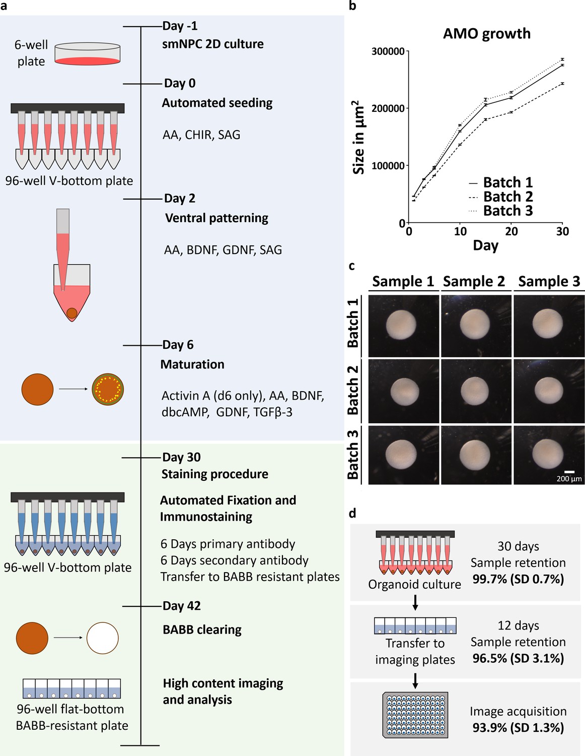
Automation enables high-throughput-compatible production and analysis of homogenous midbrain organoids.
(a) Schematic overview of the automated HTS workflow including organoid generation and optical analysis. (b) Measurement of AMO size (area of the largest cross section) reveals low variation and parallel growth kinetics for three batches of AMOs from independently thawed and cultured cells. Error bars represent standard error of the mean (SEM), n ≥ 20 organoids per data point. (c) Light microscopy images illustrating the morphological homogeneity of AMOs at day 30 of differentiation. Scale bar: 200 μm (d) Overview of sample retention at each step of processing. The automated workflow is highly efficient with 99.7% (standard deviation 0.7%) of wells retaining organoids after 30 days of culture. After whole mount staining, 96.5% (standard deviation 3.1%) of samples are successfully transferred to flat bottom imaging plates by the automated liquid handling system. This step can also be repeated without any harm to the samples to further increase efficiency. Finally, 93.9% (standard deviation 1.3%) of samples acquired by the high-content confocal microscope pass image analysis quality control and can be used for downstream analysis. SD = Standard deviation, nCulture = 30, nTransfer = 6, and nImaging = 3 96-well plates, for a list of the complete source data used to calculate the sample retention efficiency see Supplementary file 1. Also see Figure 1—figure supplement 1.
Figure 1—figure supplement 1
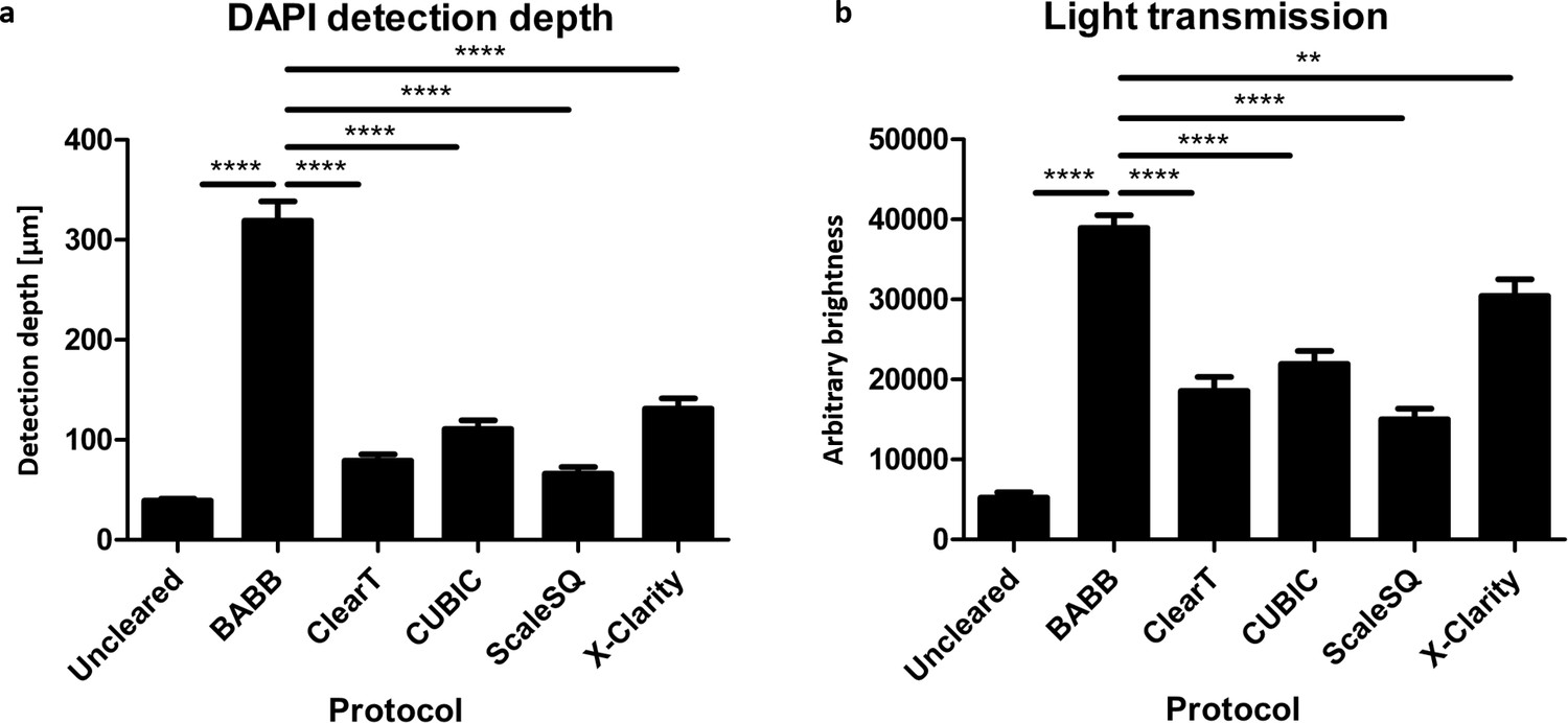
Benzyl alcohol and benzyl benzoate (BABB) tissue clearing of organoids is significantly more effective than other protocols.
(a) BABB clearing enables the detection of fluorescent signals like DAPI by confocal microscopy approximately three times deeper in organoids than other clearing protocols. (Error bars = SEM, n = 10 aggregates). (b) Organoids cleared with BABB are also significantly less opaque and more permeable to light than those cleared with other protocols. (Error bars = SEM, n = 10, X-Clarity n = 6 aggregates, **p<0.01, ****p<0.0001).
Figure 2 with 3 supplements
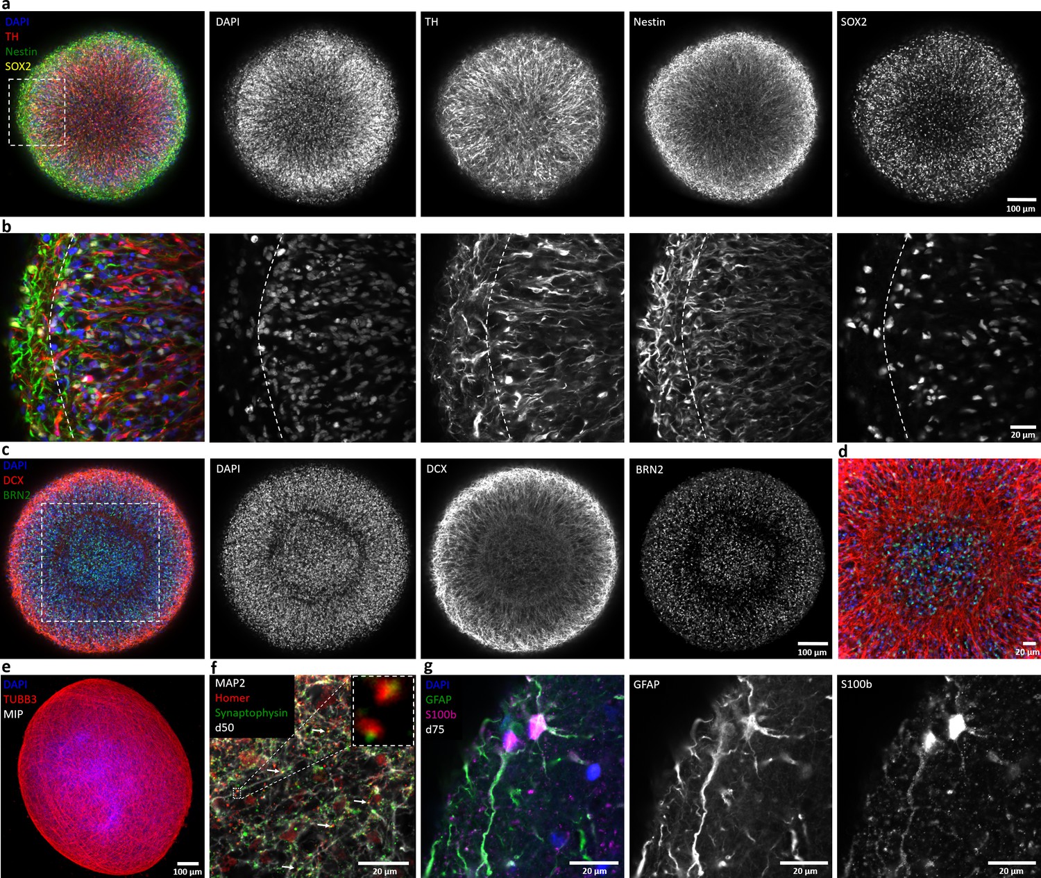
Automated midbrain organoids express typical neural and midbrain markers and show signs of structural organization.
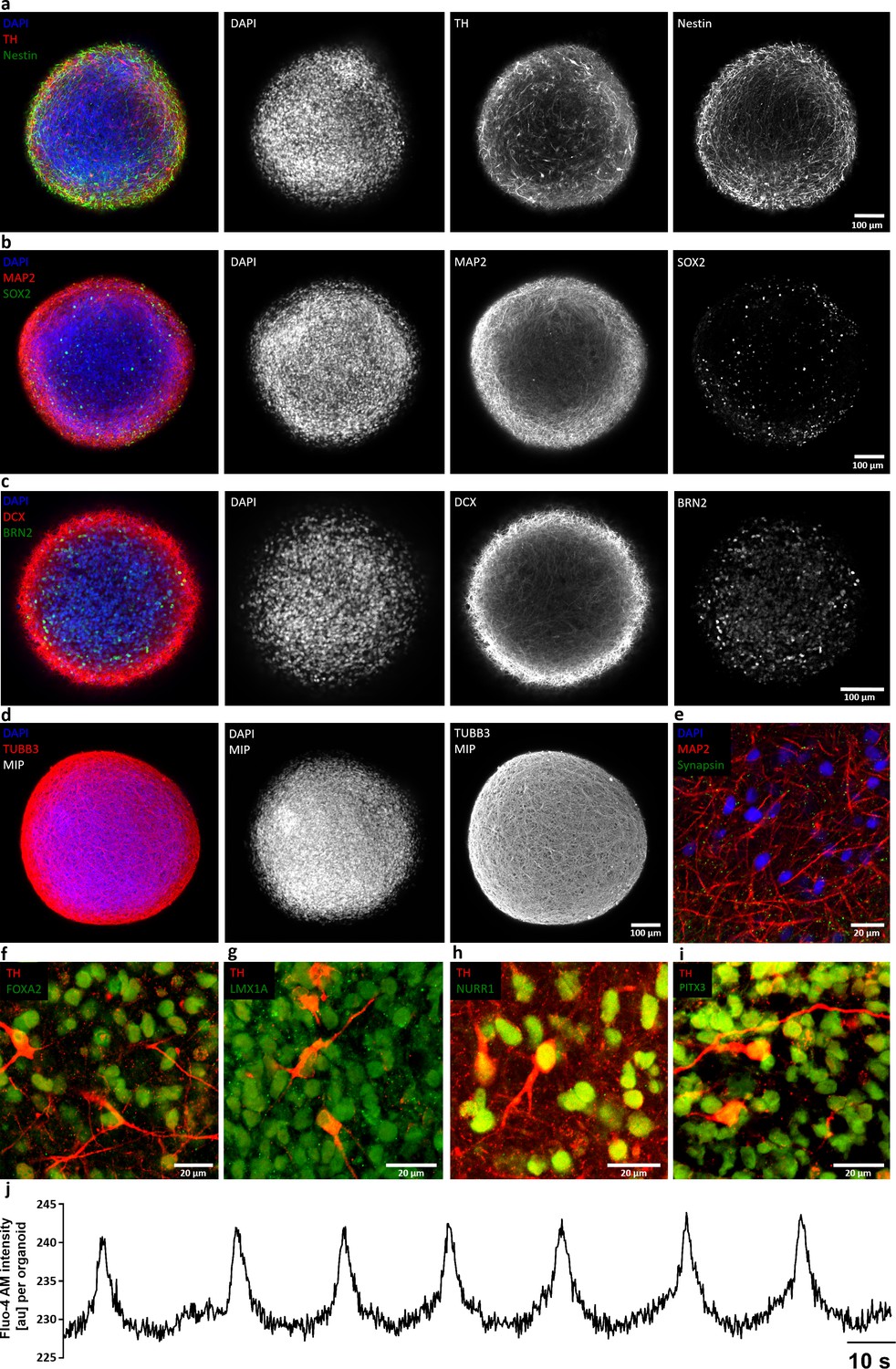
(a) Expression of the dopaminergic midbrain marker TH as well as the precursor markers nestin and Sox2 is evenly distributed throughout the entire aggregate at day 25, as shown by single confocal microscopy slices of tissue-cleared samples. The dotted box indicates the area shown in (b). Here, higher magnification of the peripheral aggregate region reveals two different zones with few nuclei but dense, circumferentially oriented neurites distally from the core and radial organization of TH-positive neurons more proximally. (c) The expression patterns of DCX and Brn2 further illustrate the organization of neurons (DCX) and neural precursors (Brn2) in the core of AMOs into zones. (d) Enlargement (of the dotted box in c) highlighting the circumferential organization of neurons (DCX) surrounding the core. (e) Maximum intensity projection (MIP) of fluorescent confocal images showing a dense cellular network expressing the neural marker β-tubulin III (TUBB33) within the AMOs at d25. (f/g) Continuing maturation of AMOs is indicated by the presence of synapses marked by the colocalization of the presynaptic synaptophysin and postsynaptic homer on Map2-positive neurites at day 50 (f, top right corner showing enlargement of two synapses without the Map2 channel) and S100b/GFAP double-positive astrocytes at day 75 (g). Scale bars: 100 μm (a, c, e), 20 μm (b, d, f, g). Also see Figure 2—figure supplements 1–3.
Figure 2—figure supplement 1
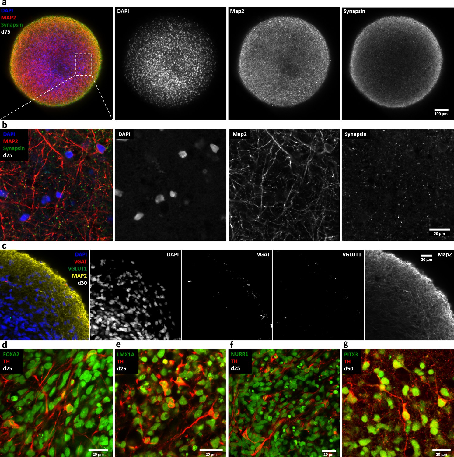
Automated midbrain organoids express synaptic and midbrain markers.
Single optical confocal slices of whole mount stained and cleared AMOs. (a/b) AMOs highly express the synaptic protein Synapsin frequently colocalizing with the neural marker Map2 (day 75). Shown in an overview (a) and in more detail (b, enlargement of the box in a) to highlight the colocalization. (c) In contrast to the highly abundant dopaminergic neurons, AMOs contain low numbers of GABAeric (vGAT) and glutamatergic (vGLUT1) neurons. (d–g) Successful differentiation of the AMOs toward a dopaminergic midbrain-like phenotype is indicated by the coexpression of typical midbrain markers including Foxa2 (d, day 25), Lmx1a (e, day 25), Nurr1 (f, day 25), and Pitx3 (g, day 50) together with the dopaminergic marker TH. Scale bars: 100 μm (a), 20 μm (b–g).
Figure 2—figure supplement 2
Characterization of AMOs generated from a second, independent patient iPSC-derived smNPC line.
(a-i) AMOs derived from a second smNPC line (AMO line 2) express the same neural precursor, neuron/synaptic, and midbrain markers as AMO line 1 (compare to Figure 2 and Figure 2—figure supplement 1). Neural precursors: Nestin (a), Sox2 (b), Brn2 (c); neurons and synapses: Map2 (b, e), DCX (c), TUBB3 (d), synapsin (e); midbrain: TH (a, f–i), FoxA2 (f), Lmx1a (g), Nurr1 (h), Pitx3 (i). All stainings were carried out after 30 days of differentiation and show either single optical confocal slices from whole mount samples or in the case of (d) maximum intensity projections (MIP). Scale bars: 100 μm (a–d), 20 μm (e–i). (j) Representative line graph of spontaneous and periodic bursts of calcium activity indicating functional coupling of the entire aggregate of AMOs from line 2 (compare to Figure 4). Experiment carried out at day 40 of differentiation on five organoids with similar outcome, recorded on a standard plate reader.
Figure 2—figure supplement 3
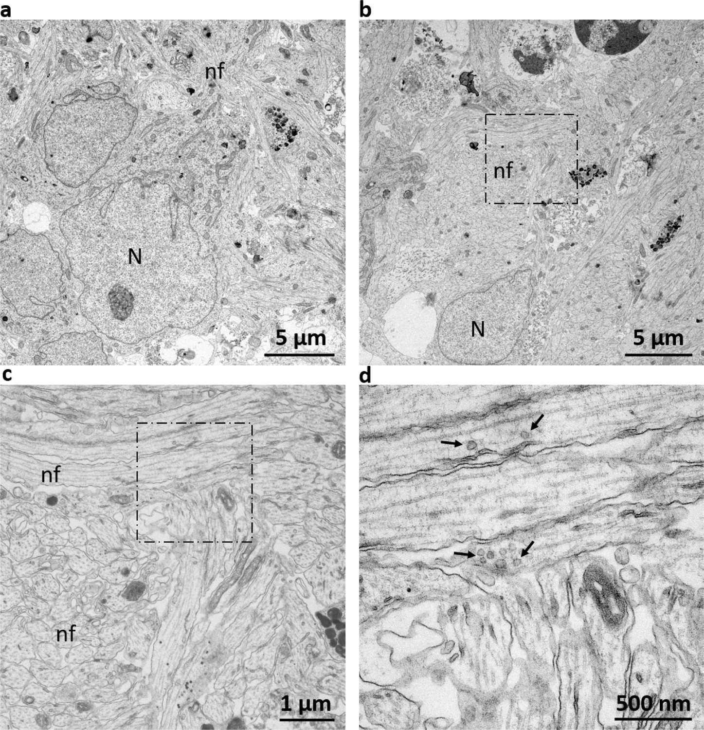
Electron microscopy displays ultrastructural morphology of neuronal phenotypes.
(a/b) Ultrastructural analysis of AMOs reveals a dense lattice of neuronal cells. The neuronal cell bodies are frequently surrounded by cellular projections commensurate with nerve fibers. (c) Enlargement of the dashed box in (b). AMOs contain bundles of nerve fibers with regularly spaced neurofilaments and microtubules resembling those of dendrites. (d) Enlarged portion marked by the dashed box in (c) showing vesicles with the characteristic size and localization of synaptic vesicles within the nerve fibers. N: Nucleus of a neural cell, nf: nerve fiber, arrows indicate synaptic vesicles. (Representative views of one example from a total of n = 3 AMOs at day 32).
Figure 3 with 1 supplement
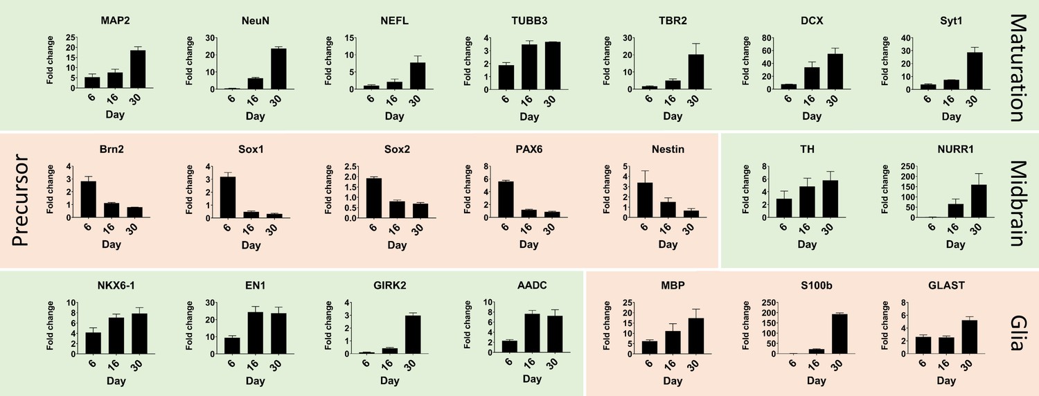
Quantitative real-time PCR shows maturation of automated midbrain organoids over time.
Changes in gene expression during the development of AMOs shown by qPCR. AMO's continuing maturation is indicated by the increase of neural maturation (MAP2, NeuN, NEFL, TUBB3, TBR2, DCX, Syt1), midbrain (TH, NURR1, NKX6-1, EN1, GIRK2, AADC), and glia (MBP, S100b, GLAST) as well as the decrease of neural precursor (Brn2, Sox1, Sox2, Pax6, nestin) markers over time. (n = 3, error bars = SEM). Also see Figure 3—figure supplement 1.
Figure 3—figure supplement 1
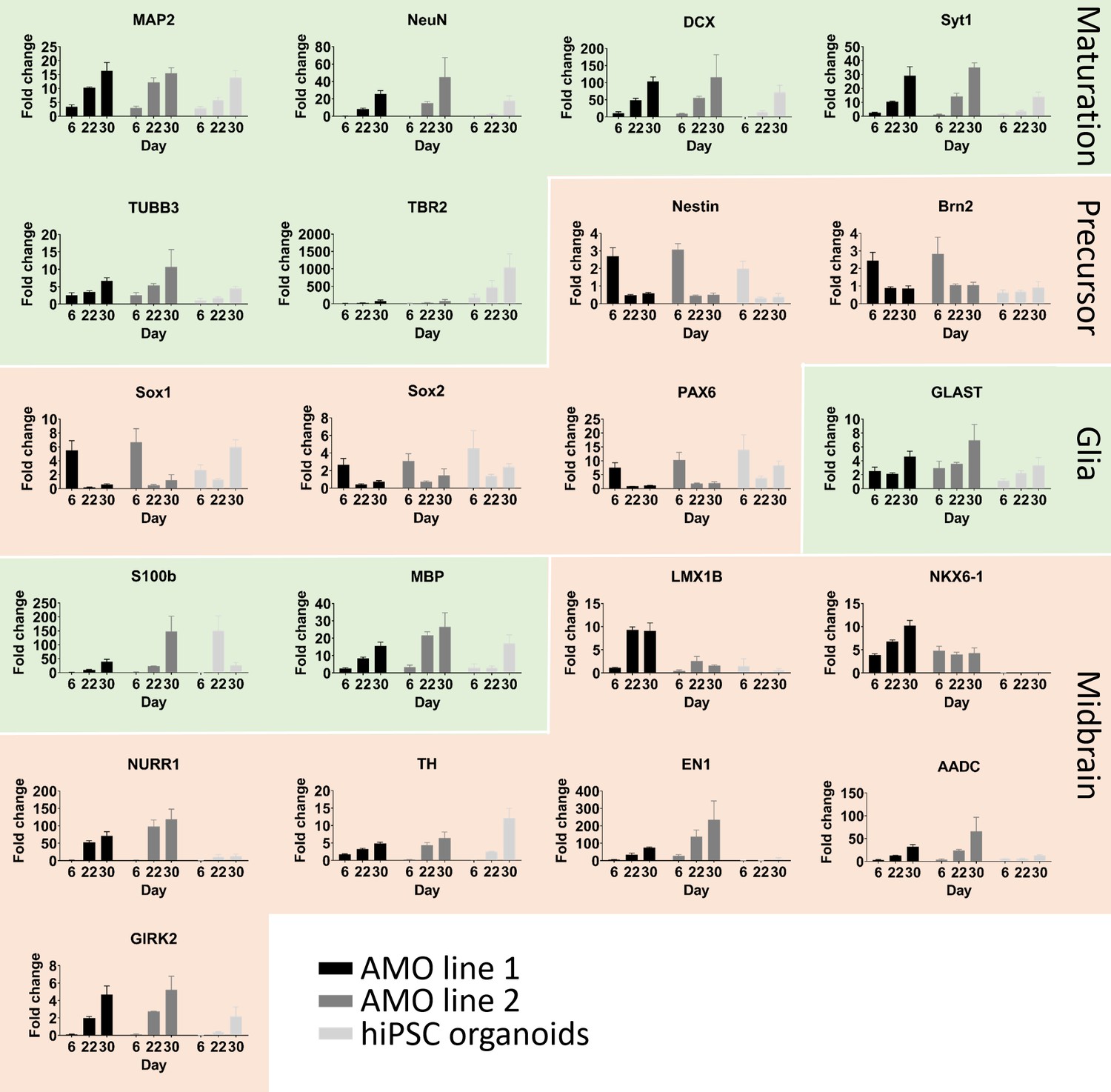
Comparative quantitative real-time PCR analysis between AMOs from two different cell lines and hiPSC organoids confirms correct differentiation toward their respective fates.
Changes in gene expression during the development of AMOs and hiPSCs shown by qPCR. Their continuing maturation is indicated by the increase of neural maturation (MAP2, NeuN, NEFL, TUBB3, TBR2, DCX, Syt1) and glia (MBP, S100b, GLAST) as well as the decrease of neural precursor (Brn2, Sox1, Sox2, Pax6, Nestin) markers over time. Consistent with their respective brain-region-specific fates, hiPSC organoids display higher expression of the more cortical marker TBR2, while the midbrain specific markers are more highly expressed in the two AMO lines (n = 3, except GIRK2 day six for the hiPSC organoids n = 2, error bars = SEM).
Figure 4 with 1 supplement
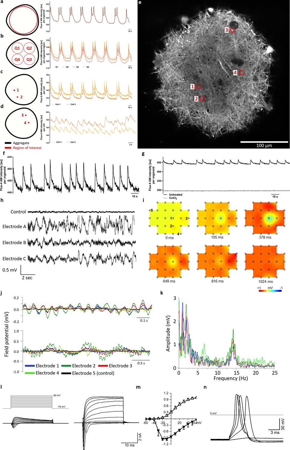
Calcium imaging reveals spontaneous and synchronized activity throughout entire organoids.
(a) AMOs show spontaneous, aggregate-wide spikes of calcium activity. (b) Division of the optical cross-section into quadrants shows that this calcium activity is occurring synchronously throughout the entire aggregate. (c) This synchronous activity pattern can be found down to the level of single spots. (d) Even distant active regions show additional levels of synchronized activity faster than the aggregate-wide spikes. (e) Single tangential fluorescent confocal slice indicating the position of spots measured in (c and d), also illustrating the dense network of active cells within the AMOs (day 93). For calcium dynamics, please refer to Video 2. Scale bar = 100 μm. (f/g) Calcium dynamics with similar activity patterns could also be detected in younger (day 35) AMOs using only a standard plate reader. Treatment with cobalt(II) chloride (CoCl2) completely abolished these spikes. (h) Spontaneous electrical activity of an AMO recorded via MEA at three electrodes (a–c) in the vicinity of the aggregate compared to background activity at a distant electrode (control). All MEA recordings were done with AMOs differentiated for 35 days and n = 3. (i) Field potential map of an AMOshowing the active area and location of electrodes. The distance between electrodes is 300 μm. (j) The field potentials recorded at electrodes 1–4 (j) form synchronous electrical waves at 14 Hz (upper panel) and 1 Hz (lower panel). (k) Fast Fourier Transformation (FFT) based on the data shown in j. (l) Representative recordings of transmembrane currents from two different cells elicited by stepping the membrane potential from −70 to +60 mV in 10 mV increments (schematic of stimulation in the left panel above). The scale bar is common for both recordings, AMOs at day 198. (m) Normalized current-voltage relationship of inward (at peak) and outward (at the end of voltage step) components of transmembrane currents averaged for all neuron-like cells (n = 29). (n) Representative recording of evoked AP’s in response to current injections from the cell shown in (l) on the right. Also see Figure 4—figure supplement 1 and Figure 2—figure supplement 2.
Figure 4—figure supplement 1
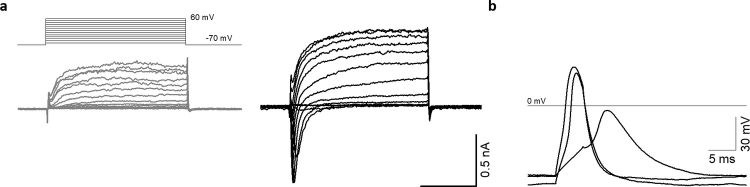
AMOs display typical neuron-like electrical activity as early as day 25.
(a) Representative recordings of transmembrane currents elicited by stepping the membrane potential from −70 to +60 mV in 10 mV increments (the schematic of stimulation is in the left panel above). Shown are one neuronal (black) and one non-neuronal (grey) cell of a 25 days old AMO. The scale bar is identical for both recordings. (b) Evoked action potentials from the neuronal cell shown in (a).
Figure 5 with 1 supplement

RNA sequencing supports differentiation toward a human midbrain-like fate and homogeneous, predictable gene expression of automated midbrain organoids.
(a/b) The global gene expression of AMOs correlates with that of fetal human brain and spinal cord tissue (a) as well as published midbrain organoids, 2D dopaminergic (DA) neurons, and prenatal midbrain (b). Shown are heatmaps of the correlation between RNA sequencing data from three independent batches of AMOs and published data sets from either 21 fetal tissues (Roost et al., 2015) (a) or of midbrain(-like) origin (Jo et al., 2016) (b). (c) AMOs from three independent batches cluster more closely together than published iPSC-derived midbrain organoids (Jo et al., 2016) in a PCA plot based on RNA sequencing data. There is no apparent difference between AMOs from the outside or inside of the plate. n = 8, except n1 outside = 18, n1 inside = 30, and niPSC midbrain organoids = 6. (d). GO term analysis reveals that most genes upregulated in the AMOs (compared to the published midbrain organoids from (b) and (c), with log2 fold change > 2) are related to neuronal and synaptic activity. Visualization via REVIGO (Supek et al., 2011), grouping GO terms based on semantic similarity. Each GO term is represented by a circle where the circle size indicates the number of genes included in the term and colors show the significance of enrichment of the term. Also see Figure 5—figure supplement 1.
Figure 5—figure supplement 1
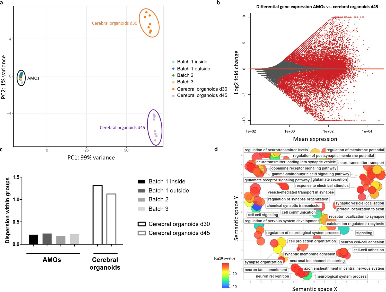
RNA sequencing reveals less intra- and inter-batch variability in AMOs compared to established cerebral organoids.
(a) AMOs from three independently cultured batches cluster more closely together than iPSC-derived cerebral organoids from one batch derived according to the protocol by Lancaster et al., 2013 in a PCA plot based on RNA sequencing data. There is no apparent difference between AMOs from the outside or inside of the plate. n = 8, except n1 outside = 18 and n1 inside = 30. (b) Differential gene expression between day 30 AMOs and day 45 cerebral organoids. The genes upregulated in AMOs (log2 fold change > 2) were used for a GO term analysis in (d). (c) Quantification of the dispersion within the different groups in the PCA plot reveals approximately six times lower variance for AMOs compared to the cerebral organoids. (d). GO term analysis reveals that most genes upregulated in the AMOs were related to neuronal maturation, especially synaptic activity. Visualization via REVIGO (Supek et al., 2011), grouping GO terms based on semantic similarity. Each GO term is represented by a circle where the circle sizes indicates the number of genes included in the term and colors show the significance of enrichment of the term.
Figure 6 with 1 supplement
Automated whole mount immunostaining is quantitative and reveals high homogeneity of automated midbrain organoids.
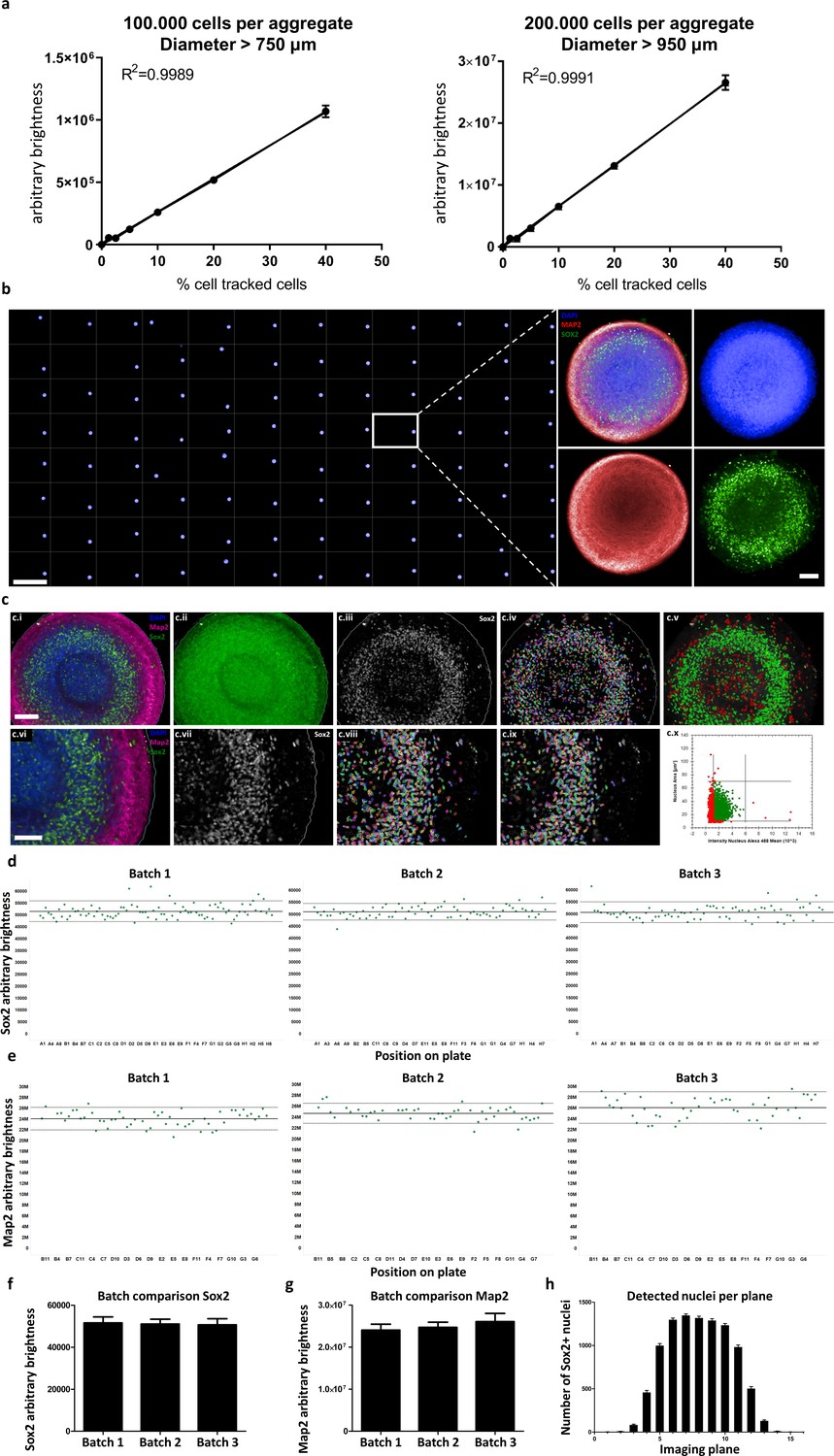
(a) The optical analysis workflow allows quantification of cell numbers in 3D aggregates. The correlation between the number of fluorescent cells in an aggregate and its brightness measured with our workflow is highly linear (R2 > 0.99) for large-scale 3D aggregates of different sizes (100,000 or 200,000 cells per aggregate, diameter > 750 μm and 950 μm, respectively). n = 3, error bars = SEM. (b) Overview of an entire 96-well plate processed with our HTS-compatible optical analysis workflow (left) and an example single plane confocal image of a single AMO illustrating the high cellular resolution achieved with high-content imaging (right). Scale bars: 5 mm left/overview; 100 μm right/enlargement. (c) Visualization of the automated image analysis sequence for the example of Sox2. Images show a single automatically acquired confocal image plane through the center of an AMO. Top row: Overview, with bottom row providing enlarged view. (c.i/vi) Starting image. (c.ii) All three channels summed for aggregate detection. Detected aggregate area overlaid in green. (c.iii/vii) Sox2 channel after sliding parabola treatment to remove background. (c.iv/viii) Sox2 channel with detected nuclei. (c.v) Nuclei selected as Sox2+ according to size and brightness (green) and rejected nuclei (red). (c.ix) Selected nuclei from (h) marked, rejected nuclei unmarked. (c.x) Scatter plot showing nuclear size and brightness distribution and selection thresholds. Scale bars: 100 μm (c.i), top row; 70 μm (c.vi), bottom row. (d–g) AMOs are homogenous with regard to the amount of Sox2 (d/f) and Map2 (e/g) positive cells they contain. In (d and e) each dot represents a single AMO, each graph originating from an independent batch (i.e. cells were separately thawed, cultured and processed). The continuous line represents the mean of all data points on the graph (i.e. Map2/Sox2 content) and the dotted lines correspond to 1.5 confidence intervals. (f and g) Summarize the data of the dot plots as a bar graph. (Error bars = standard deviation, SD). (h) The number of Sox+ nuclei detected in each imaged confocal plane correlates with AMO morphology. The high-content image analysis workflow detects many nuclei where the aggregate diameter is largest (plane 6–10) and fewer nuclei in the first/last planes where it is smaller. (Error bars = SEM). Also see Figure 6—figure supplement 1.
Figure 6—figure supplement 1
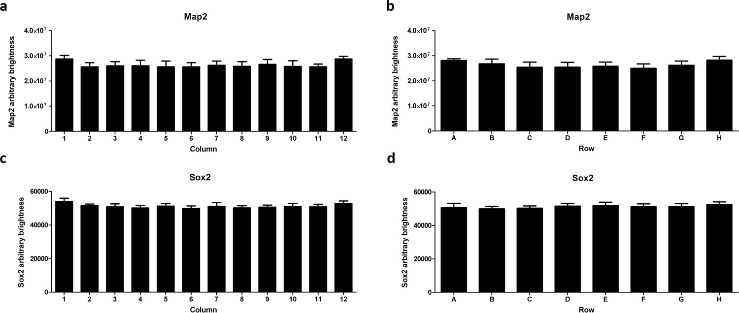
High-content imaging analysis reveals edge effects for Map2 but not Sox2.
AMOs on the edge of the plate (column 1 and 12 in a) and row A and H in (b) contain approximately 10% more Map2 (by brightness) than the ones more toward the inside of the plate. For Sox2, there is a slight difference of approximately 5% in total summed brightness between the inside and the two outmost columns of the plate (c) but none for the rows (d).
Figure 7 with 2 supplements
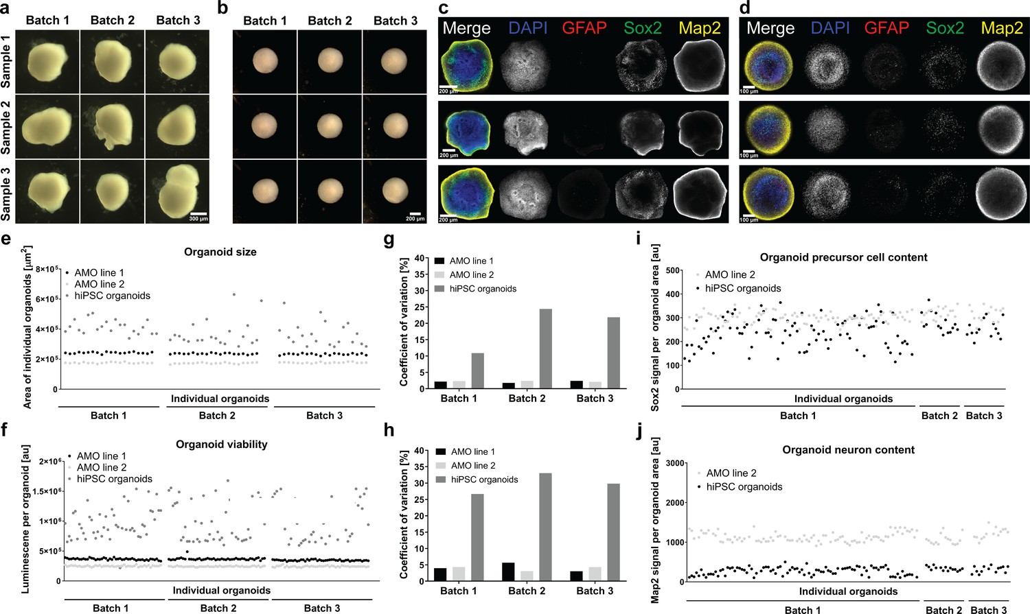
smNPC-derived AMOs are morphologically, structurally, and functionally more homogeneous than automated hiPSC-derived organoids.
(a/b) Light microscopy images of hiPSC-derived organoids (a) and AMOs (b) generated from the same cell line demonstrating the higher morphological homogeneity of AMOs at day 30 of differentiation.(c/d) Single optical confocal slices of either hiPSC-derived organoids (c) or AMOs (d) at day 30 stained for DAPI, the astrocyte marker GFAP, the neural precursor marker Sox2, and the neuronal marker Map2. The direct comparison illustrates the higher level of structural homogeneity as well as accelerated maturation, especially the earlier emergence of GFAP+ astrocytes in AMOs. Rows depict three samples from one batch. (e/f) Size (area of the largest cross section) and cell viability measurements of individual organoids from three independent batches (per cell line/differentiation protocol) illustrating the high homogeneity of AMOs compared to standard hiPSC organoids. (g/h) Coefficients of variation calculated based on the data shown in (e) and (f). (i/j) Quantitative whole mount staining (see also Figure 6) for Sox2 (i), and Map2 (j) showing the higher variability of hiPSC organoids compared to AMOs from the same iPSC line even after normalization to the organoid area. All data gathered from organoids at day 30 of differentiation. Scale bars: 300 μm (a), 200 μm (b/c), 100 μm (d). Also see Figure 7—figure supplements 1 and 2.
Figure 7—figure supplement 1
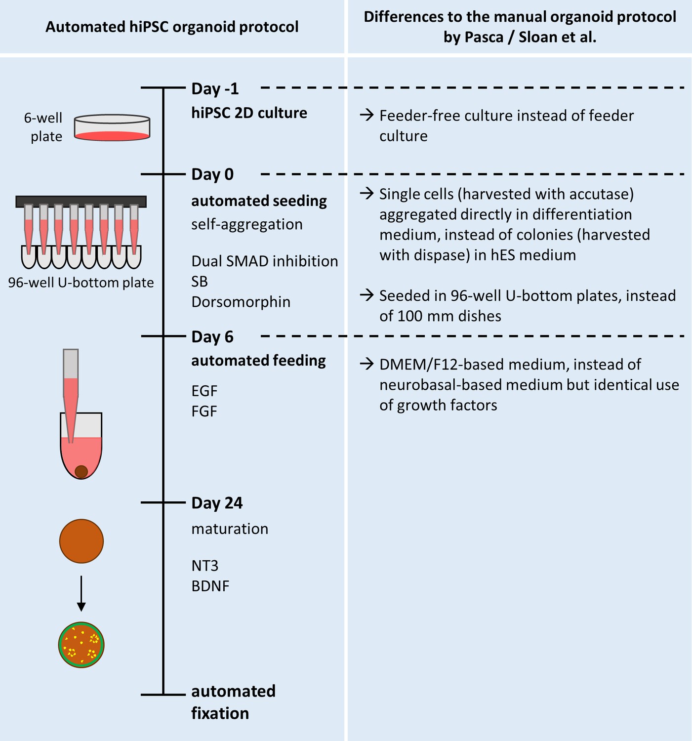
Overview of the protocol for the automated generation of hiPSC-based organoids and modifications from the published original.
Schematic overview of the automated HTS workflow for the generation and maintenance of the automated hiPSC-organoids. The right half of the Figure details the modifications made from the original protocol published by Paşca et al., 2015 (and described in more detail by Sloan et al., 2018).
Figure 7—figure supplement 2

The expression of typical neural and cortical markers confirms the correct differentiation of automated hiPSC-derived organoids.
(a/b) Single optical confocal slices of whole mount stained and tissue-cleared organoids showing the expression of the early cortical neuron marker CTIP2, precursor marker Pax6, and general neuronal marker Map2 at day 40. Expression of the different markers is generally confined to specific regions of the organoid. While Pax6 expression is highest in the neural rosette-like structures, CTIP2 is mostly found surrounding these regions (see (b) for an enlarged view of a rosette). The expression pattern of the general neuronal marker Map2 indicates that most neurons are located within the outer regions of the organoid with lower expression toward the center. (c) At day 30, staining for the forebrain precursor marker FoxG1 combined with Map2 further confirms the correct differentiation toward a cortical fate. (d/e) Consistently, the expression of the precursor markers Brn2 (d) and Sox2 (e) is mostly confined to the neural rosette-like structures, while the neural marker DCX (d) shows a distribution similar to that of Map2 in 30 days old organoids. (f/g) The precursor marker TBR2 is also mainly expressed in confined regions of the organoid surrounded by more mature cortical markers like TBR1 (f) and CTIP2 (g) at day 30 of differentiation. (h) Late-born SATB2+ neurons arise starting day 50. (i) At day 40, few synapsin-positive punctae on Map2-positive neurites indicate formation of first synapses. (j) Maximum intensity projection (MIP) showing the network of β-Tubulin III (TUBB3) positive neurons as well as Sox2-positive precursors throughout a 30 days old organoid. (k) While the mostly unguided nature of the differentiation protocol does allow for the emergence of other cell types, expression of TH is confined to a small area and limited to few cells after 40 days of differentiation. Organoids shown were at either day 30 (c, d, e, f, g, j), 40 (a, b, i, k), or 50 (h) of differentiation. Scale bars: 200 μm (a, c, d, e, f, g, h), 20 μm (b, g).
Figure 8 with 1 supplement
Automated midbrain organoids possess functional characteristics of midbrain tissue and allow assessment of neural subpopulations for high-throughput screening.
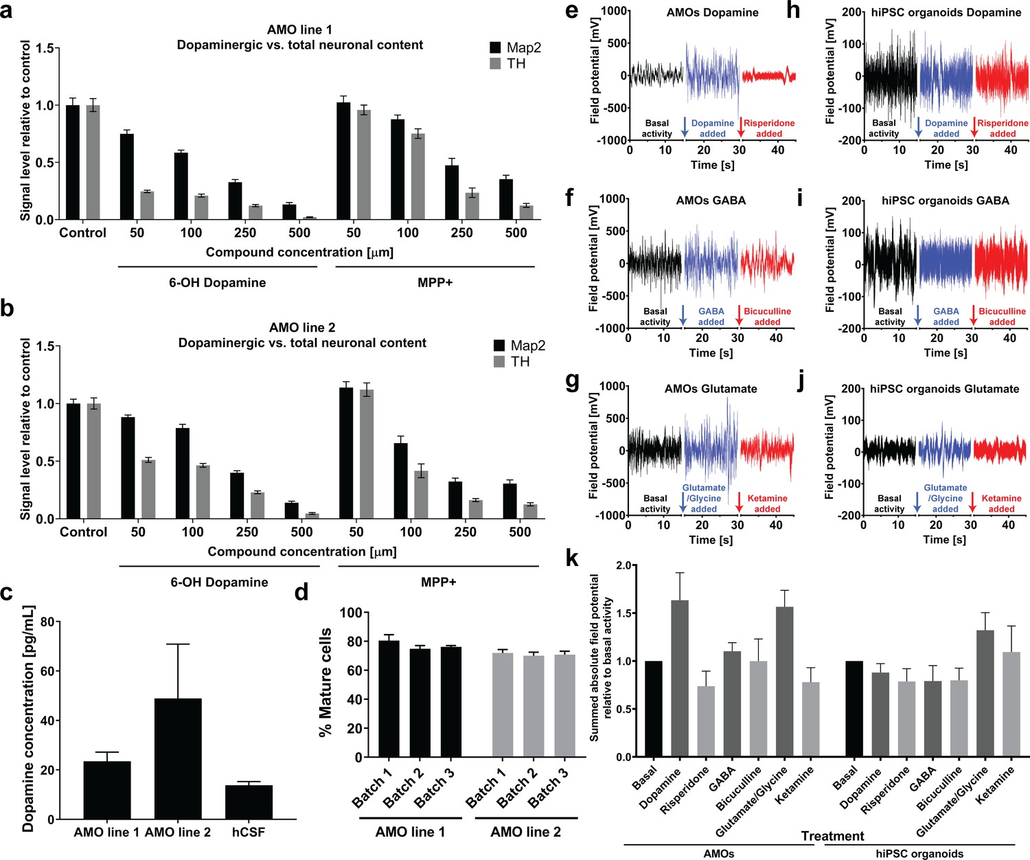
(a/b) The combination of AMOs and our automated whole mount staining and clearing workflow allows the quantification of dopaminergic neuron-specific toxicity in 3D. 6-Hydroxy dopamine and MPP+ specifically ablate TH-positive dopaminergic neurons from the AMOs in a dose-dependent manner and with little variation between replicates and cell lines. n ≥ 6 organoids per data point, Error bars: SEM. Organoids at day 56 of differentiation. (c) 35 days old AMOs secrete dopamine into their cell culture medium under standard culture conditions and without further stimulation, as confirmed by ELISA. The concentration is in the same range as the dopamine levels measured in the cerebrospinal fluid (CSF) of healthy, adult humans as reported by Goldstein et al., 2012. nLine 1 = 4, nLine 2 = 3, nhCSF = 38, Error bars: SEM. (d) 70–80% percent of cells within the AMOs are negative for the precursor marker Sox2 after 30 days of differentiation. AMO line 1: nBatch1 = 90, nBatch2 = 16, nBatch3 = 15; AMO line 2: nBatch1 = 89, nBatch2 = 16, nBatch3 = 14; Error bars: SD. (e–j) AMOs respond most strongly to dopaminergic modulation and, to a lesser extent, also to glutamatergic modulation while the automated cortical hiPSC organoids are mostly affected by compounds targeting glutamatergic neurons. MEA measurements of individual AMOs (e–g) or cortical hiPSC organoids (h–j) were performed in three stages on the same sample: first, under basal conditions (black line), second, after treatment with an agonist (blue line), and third, after addition of an antagonist (red line). The pharmacological modulators targeted dopaminergic (e/h), GABAergic (f/i), or glutamatergic (g/j) neurons. The gaps in the X-axis represent the addition of the different compounds and the time we allowed for the solution to equilibrate. Shown is the raw signal of one representative example of n = 4. AMOs were at 33 days and hiPSCs at 35 days of differentiation. (k) Quantification of the effects of pharmacological modulation on AMOs and automated hIPSC organoids as measured by MEA. The bar graph shows the sum of the absolute electric field potential oscillations over 15 s of time relative to basal conditions for each modulator. Each bar represents the mean +/- SEM for n = 4 replicates, one representative raw measurement per condition is shown in (e-j). n = 4, except nhiPSC organoids Glutamate = 3; Also see Figure 8—figure supplement 1.
Figure 8—figure supplement 1
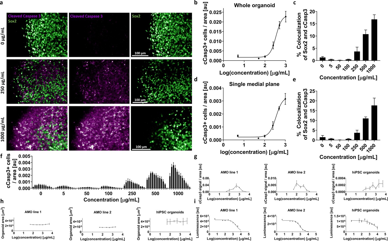
AMOs allow HTS-compatible toxicity evaluation in whole organoids or specific cellular subpopulations.
(a) Higher toxin concentrations resulted in increased cCasp3+ apoptotic signal in AMOs. Panel shows representative single plane confocal micrographs from our high-content analysis pipeline after adding G418 for 4 days starting at day 50 of culture. Scale bars = 100 μm. (b) Increase of cCasp3+ cells follows a typical sigmoidal dose-response kinetic in AMOs with escalating concentrations of G418. Depicted is the total number of cCasp3 cells per organoid normalized by the organoid area on the y-axis against the logarithmic concentration of G418 on the x-axis. n ≥ 3, error bars = SEM. (c) The cCasp3 signal shows little colocalization with Sox2, indicating that not neuronal precursors but other, more mature cell types are primarily affected by the treatment. The percentage of Sox2+ neural precursors among the apoptotic cells increased with the inhibitor concentration but remained relatively low with a maximum of approximately 15%. n ≥ 3, error bars = SEM (d/e) The dose-response curve (d) and colocalization analysis (e) based on a single plane display almost identical results to the ones based on entire organoids (b/c). This potentially allows a substantial reduction of imaging time and costs by acquiring only single medial slices instead of entire organoid volumes. n ≥ 3, error bars = SEM. (f) Bar graph showing the number of apoptotic cCasp3+ cells (normalized by area) for single confocal planes. Each bar represents one plane; bars are grouped by the concentration of the G418 treatment. n ≥ 3, error bars = SEM. (g/h) Followup high-content imaging-based evaluation of G418 toxicity with two different AMO lines and hiPSC organoids using a wider range of G418 concentrations than first tested in (a–f) illustrating the drawbacks of cCasp3-based toxicity screening. As cCasp3 labels cells only for a transient time during cell death, the peak signal can be missed and results can be misleading. Here, higher concentrations of G418 resulted in lower levels of cCasp3 positive cells after 96 hr (g). The size (area of the cross section) of the organoids from (g) did not change with increased concentrations of G418 (h). n ≥ 3, Error bars: SEM. (i) ATPglo-based cell viability measurements of G418 treated AMOs and hiPSC organoids (each from the same batch and treated together with the samples shown in (g)), confirmed that higher concentrations of G418 are indeed more toxic and the cCasp3-based readout failed to detect this effect. In all three assays (g-i) AMOs showed lower variance than hiPSC organoids. nAMO line 1&2 = 6, nhiPSC organoids ≥ 5, Error bars: SD. All samples in (g-i) were at day 35 at the time of analysis.
Videos
Video 1
The combination of whole mount staining and clearing allows confocal imaging of 3D cellular architecture at single-cell resolution.
3D rendering of a confocal stack showing the 3D organization of neural precursors (Sox2, green) and mature neurons (Map2, red) within AMOs. The video shows a cube-shaped volume with edge length of 150 µm. Nuclei were counter-stained with DAPI (blue). AMO at day 25 of differentiation.
Video 2
Automated midbrain organoids display spontaneous and aggregate-wide synchronized calcium activity.
Single plane spinning disc confocal time lapse series showing fluctuations in Fluo-4 AM fluorescence of a near-surface tangential optical slice. Images were acquired at 10 Hz for a total of 4 min. Changes are quantified in Figure 4. Representative video of n = 5 organoids with similar synchronized activity patterns.
Tables
Key resources table
| Reagent type (species) or resource | Designation | Source or reference | Identifiers | Additional information |
|---|---|---|---|---|
| Cell line (Homo sapiens) | AMO line 1 | Reinhardt et al., 2013b | PMID:23533608 | smNPCs used for the derivation of AMOs designated ‘AMO line 1’ |
| Cell line (Homo sapiens) | AMO line 2 | Reinhardt et al., 2013a | PMID:23533608 | smNPCs used for the derivation of AMOs designated ‘AMO line 2’ |
| Cell line (Homo sapiens) | hIPSCs | Reinhardt et al., 2013a | PMID:23472874; PMID:23533608 | hIPSCs giving rise to hIPSC organoids in this paper; cell line of origin to generate smNPCs for AMO line 2 |
| Antibody | Anti-Brn2 (Rabbit monoclonal) | Cell Signaling | Cat#:12137 | (1:2000) |
| Antibody | Anti-Cleaved Caspase-3 (Rabbit monoclonal) | Cell Signaling | Cat#:9664 | (1:100) |
| Antibody | Anti-Ctip2 (Rat monoclonal) | Abcam | Cat#:ab18465 | (1:750) |
| Antibody | Anti-DCX (Goat polyclonal) | Santa Cruz | Cat#:sc-8066 | (1:500) |
| Antibody | Anti-FoxA2 (Mouse monoclonal) | Santa Cruz | Cat#:sc-101060 | (1:100) |
| Antibody | Anti-FoxG1 (Rabbit polyclonal) | Abcam | Cat#:ab18259 | (1:500) |
| Antibody | Anti-GFAP (Chicken polyclonal) | Merck Millipore | Cat#:AB5541 | (1:500) |
| Antibody | Anti-Lmx1a (Rabbit polyclonal) | Abcam | Cat#:ab139726 | (1:100) |
| Antibody | Anti-Homer (Mouse monoclonal) | Synaptic Systems | Cat#:160 011 | (1:250) |
| Antibody | Anti-Map2 (Chicken polyclonal) | Abcam | Cat#:ab5392 | (1:500) |
| Antibody | Anti-Map2 (Mouse monoclonal) | Merck Millipore | Cat#:MAB3418 | (1:1000) |
| Antibody | Anti-Map2 (Rabbit polyclonal) | Abcam | Cat#:ab32454 | (1:500) |
| Antibody | Anti-Nestin (Mouse monoclonal) | Life Technologies | Cat#:MA1-110 | (1:250) |
| Antibody | Anti-Nurr1 (Mouse monoclonal) | Santa Cruz | Cat#:sc-376984 | (1:100) |
| Antibody | Anti-Pax6 (Rabbit polyclonal) | BioLegend | Cat#:901301 | (1:500) |
| Antibody | Anti-Pitx3 (Rabbit polyclonal) | Merck Millipore | Cat#:AB5722 | (1:100) |
| Antibody | Anti-S100b (Rabbit polyclonal) | Dako | Cat#:Z031129-2 | (1:500) |
| Antibody | Anti-Satb2 (Mouse monoclonal) | Abcam | Cat#:ab51502 | (1:500) |
| Antibody | Anti-Sox2 (Goat polyclonal) | R and D Systems | Cat#:AF2018 | (1:200) |
| Antibody | Anti-Synapsin1 (Mouse monoclonal) | Synaptic Systems | Cat#:106 001 | (1:1000) |
| Atibody | Anti-Synaptophysin1 (Rabbit polyclonal) | Synaptic Systems | Cat#:101 002 | (1:200) |
| Antibody | Anti-Tbr1 (Rabbit polyclonal) | Abcam | Cat#:ab31940 | (1:500) |
| Antibody | Anti-Tbr2 (Chicken polyclonal) | Merck Millipore | Cat#:AB15894 | (1:500) |
| Antibody | Anti-TUBB3 (Mouse monoclonal) | BioLegend | Cat#:801202 | (1:500) |
| Antibody | Anti-TH (Chicken polyclonal) | Abcam | Cat#:ab76442 | (1:1000) |
| Antibody | Anti-TH (Rabbit polyclonal) | Abcam | Cat#:ab112 | (1:500) |
| Antibody | Anti-vGAT (Mouse monoclonal) | Synaptic Systems | Cat#:131 011 | (1:100) |
| Antibody | Anti-vGLUT1 (Rabbit polyclonal) | Synaptic Systems | Cat#:135 303 | (1:100) |
| Sequence-based reagent | AADC_F | This paper | PCR primers | TGCGAGCAGAGAGGGAGTAG |
| Sequence-based reagent | AADC_R | This paper | PCR primers | TGAGTTCCATGAAGGCAGGATG |
| Sequence-based reagent | Brn2_F | This paper | PCR primers | CGGCGGATCAAACTGGGATTT |
| Sequence-based reagent | Brn2_R | This paper | PCR primers | TTGCGCTGCGATCTTGTCTAT |
| Sequence-based reagent | DCX_F | This paper | PCR primers | AGGGCTTTCTTGGGTCAGAGG |
| Sequence-based reagent | DCX_R | This paper | PCR primers | GCTGCGAATCTTCAGCACTCA |
| Sequence-based reagent | EN1_F | This paper | PCR primers | CCCTGGTTTCTCTGGGACTT |
| Sequence-based reagent | EN1_R | This paper | PCR primers | GCAGTCTGTGGGGTCGTATT |
| Sequence-based reagent | GAPDH_F | This paper | PCR primers | CTGGTAAAGTGGATATTGTTGCCAT |
| Sequence-based reagent | GAPDH_R | This paper | PCR primers | TGGAATCATATTGGAACATGTAAACC |
| Commercial assay or kit | Biomark 48.48integrated fluidic circuit Delta Gene assay | Fluidigm | Cat#:101–0348 | Complete bundle for 10 assays |
| Commercial assay or kit | CellTiter-Glo 3D Cell Viability Assay | Promega | Cat#:G9682 | |
| Commercial assay or kit | Dopamine ELISA Kit | Abnova | Cat#:KA3838 | |
| Commercial assay or kit | CellTracker deep red dye | Life Technologies | Cat#:C34565 | |
| Commercial assay or kit | Fluo-4 AM | Thermo Fisher | Cat#:F14201 | |
| Chemical compound, drug | Cobalt(II) chloride | Sigma-Aldrich | Cat#:232696 | |
| Chemical compound, drug | G418 | Sigma-Aldrich | Cat#:G8168 | |
| Chemical compound, drug | 6-Hydroxydopamine hydrochloride (6OHD) | Sigma-Aldrich | Cat#:H4381 | |
| Chemical compound, drug | 1-Methyl-4-phenylpyridinium iodide (MPP+) | Sigma-Aldrich | Cat#:D048 | |
| Chemical compound, drug | Dopamine hydrochloride | Sigma-Aldrich | Cat#:H8502 | |
| Chemical compound, drug | Risperidone | Sigma-Aldrich | Cat#:R3030 | |
| Chemical compound, drug | GABA | Sigma-Aldrich | Cat#:A2129 | |
| Chemical compound, drug | Bicuculline | Sigma-Aldrich | Cat#:14340 | |
| Chemical compound, drug | Glutamate | Sigma-Aldrich | Cat#:49621 | |
| Chemical compound, drug | Glycine | Sigma-Aldrich | Cat#:50046 | |
| Chemical compound, drug | Ketamine | Sigma-Aldrich | Cat#:K2753 | |
| Software, algorithm | Fiji | Schindelin et al., 2012 | PMID:22743772 | |
| Software, algorithm | GraphPad Prism | Graphpad Software Inc | RRID:SCR_002798 | |
| Software, algorithm | Harmony | Perkin Elmer | Version:‘4.1, Revision 128972’ | |
| Software, algorithm | Columbus | Perkin Elmer | Version:2.6.0.127073 |
Additional files
-
Supplementary file 1
Source data for the calculation of sample retention efficiency shown in Figure 1d.
- https://cdn.elifesciences.org/articles/52904/elife-52904-supp1-v1.docx
-
Supplementary file 2
Complete List of gene ontology (GO) terms for genes significantly (p<0.001) upregulated (log2 fold change >2) in AMOs compared to published midbrain organoids (Jo et al., 2016).
- https://cdn.elifesciences.org/articles/52904/elife-52904-supp2-v1.docx
-
Supplementary file 3
List of primary antibodies in this study.
- https://cdn.elifesciences.org/articles/52904/elife-52904-supp3-v1.docx
-
Supplementary file 4
List of quantitative real-time PCR primers in this study.
- https://cdn.elifesciences.org/articles/52904/elife-52904-supp4-v1.docx
-
Transparent reporting form
- https://cdn.elifesciences.org/articles/52904/elife-52904-transrepform-v1.docx
Download links
A two-part list of links to download the article, or parts of the article, in various formats.
Downloads (link to download the article as PDF)
Open citations (links to open the citations from this article in various online reference manager services)
Cite this article (links to download the citations from this article in formats compatible with various reference manager tools)
A fully automated high-throughput workflow for 3D-based chemical screening in human midbrain organoids
eLife 9:e52904.
https://doi.org/10.7554/eLife.52904


