Cerebellar patients have intact feedback control that can be leveraged to improve reaching
- Kennedy Krieger Institute, United States
- Department of Biomedical Engineering, Johns Hopkins University, United States
- Department of Mechanical Engineering and Laboratory for Computational Sensing and Robotics, Johns Hopkins University, United States
- Department of Neuroscience, Johns Hopkins University, United States
Figures
Figure 1
The experimental paradigm.
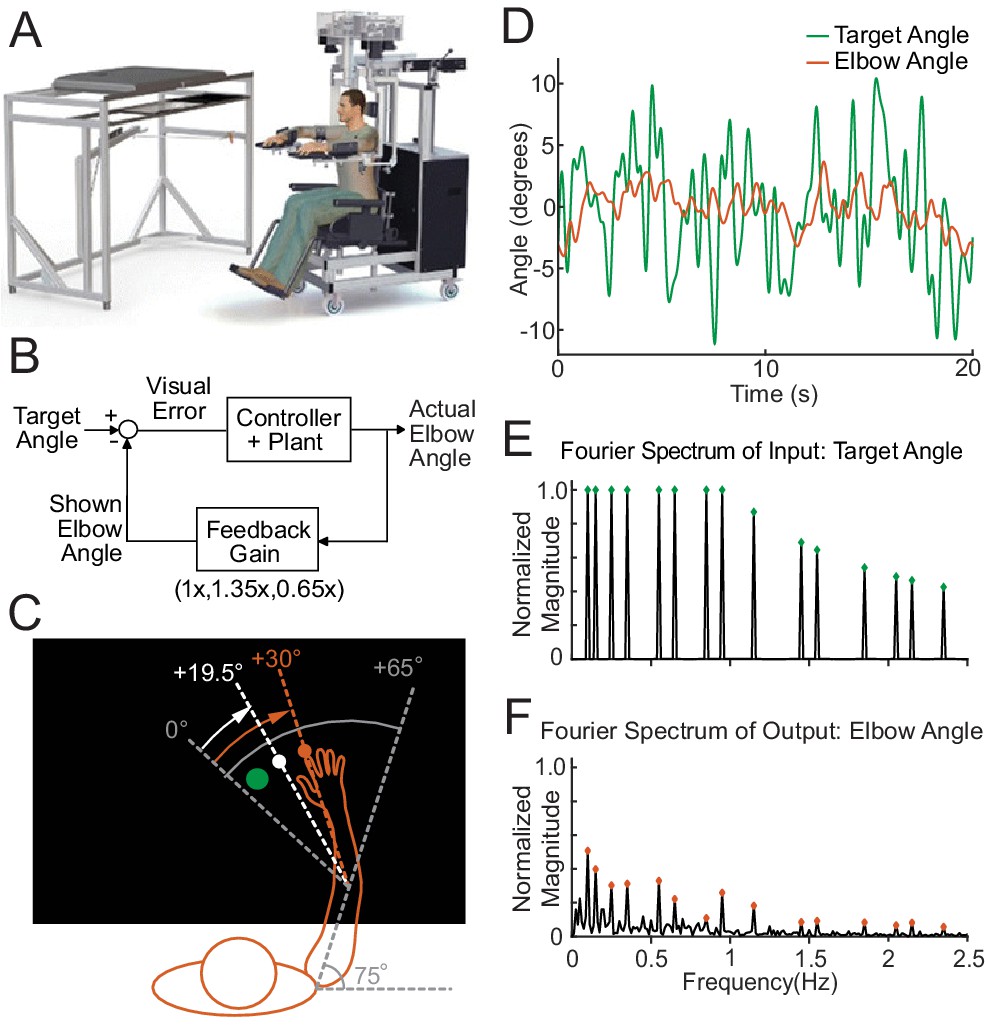
(A) The Kinarm Exoskeleton robot system (BKIN Technologies Ltd.) where all tasks are executed. Image is taken from Tyryshkin et al., 2014. (B) This block diagram shows our experimental paradigm for experiment 1. The actual elbow angle (orange in C) is multiplied by a feedback gain to compute the shown elbow angle (white dot in C). (C) A schematic view of the Kinarm screen in the 0.65 Feedback Gain condition. The subject's shoulder is locked at a 75° angle. The green dot is the target dot. The green dot oscillates according to the sum-of-sines pattern along an arc with a radius equivalent to the forearm + hand + finger length. The sum-of-sines pattern is centered about the 0° angle. This 0° centerline is at a 65° angle from the subject's straight arm position. The subject could not see their fingertip (orange dot) or arm position. The angle of the white dot (visible to the subject) is equal to 0.65 times the actual fingertip angle in orange (0.65 ⋅ 30°=19.5°). (D) Sample data (20 s) for a single cerebellar patient showing the angles traversed by the target dot during the sum-of-sines task (green) and by the fingertip (orange, averaged over five trials). (E) The normalized Fourier spectrum of the input sum-of-sines signal (green trace in D). (F) The spectrum of the response by a single cerebellar patient over five trials (orange trace in D).
Figure 2
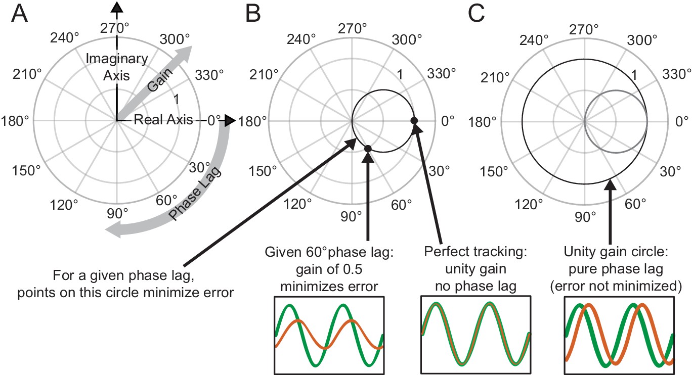
Interpreting phasor plots.
(A–C) Brief explanation of phasor plots, which are explained in depth in Methods in ‘Phasor Plot.’ (A) Illustration of the relationship between the real and imaginary components of the complex numbers and the gain and phase lag. (B) The bold black circle illustrates the gains that minimize error given a particular phase lag (veridical feedback condition only). (C) Points on the bold black circle illustrate a different control strategy than what was asked of our subjects. Points on this circle replicate the input signal without minimizing error between the input and output signals (veridical feedback condition only) due to the phase lag.
Figure 3
Motion rescaling under different feedback gains.
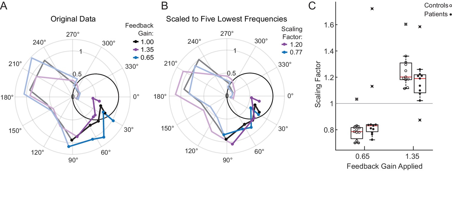
(A) Sample phasor plot data from a single cerebellar patient under all three feedback gain conditions. The dots represent the frequency response at the lowest five frequencies. The solid line traces through the responses at all tested frequencies. The dimmed lines show the frequency responses at the other frequencies tested beyond the five lowest frequencies. (B) Scaled phasor plot data from the same single cerebellar patient. The gain value from D has been multiplied by the scaling factor shown in the legend here to create an overlaid phasor plot. The higher the Scaling Factor, the less effort (in terms of movement magnitude) the subject expended in that condition. (C) Patients and controls respond similarly to the applied Feedback Gain, indicating that they incorporate visual feedback similarly. The higher the Scaling Factor, the less effort (in terms of movement magnitude) the subject expended in that condition. Outliers are marked with an x. The outlier subject with the highest Scaling Factor in the 0.65 condition was from the same subject who had the lowest Scaling Factor in the 1.35 condition.
Figure 4 with 2 supplements
Modeling.
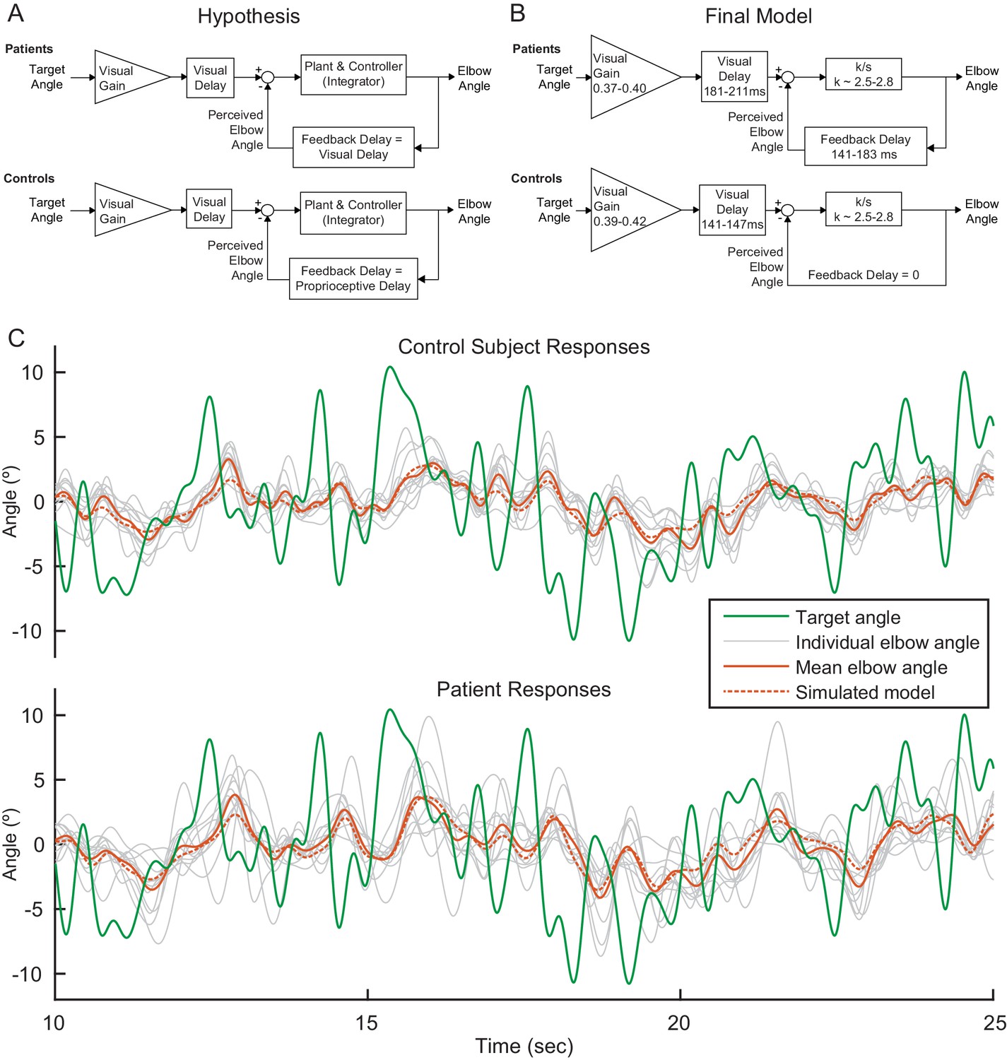
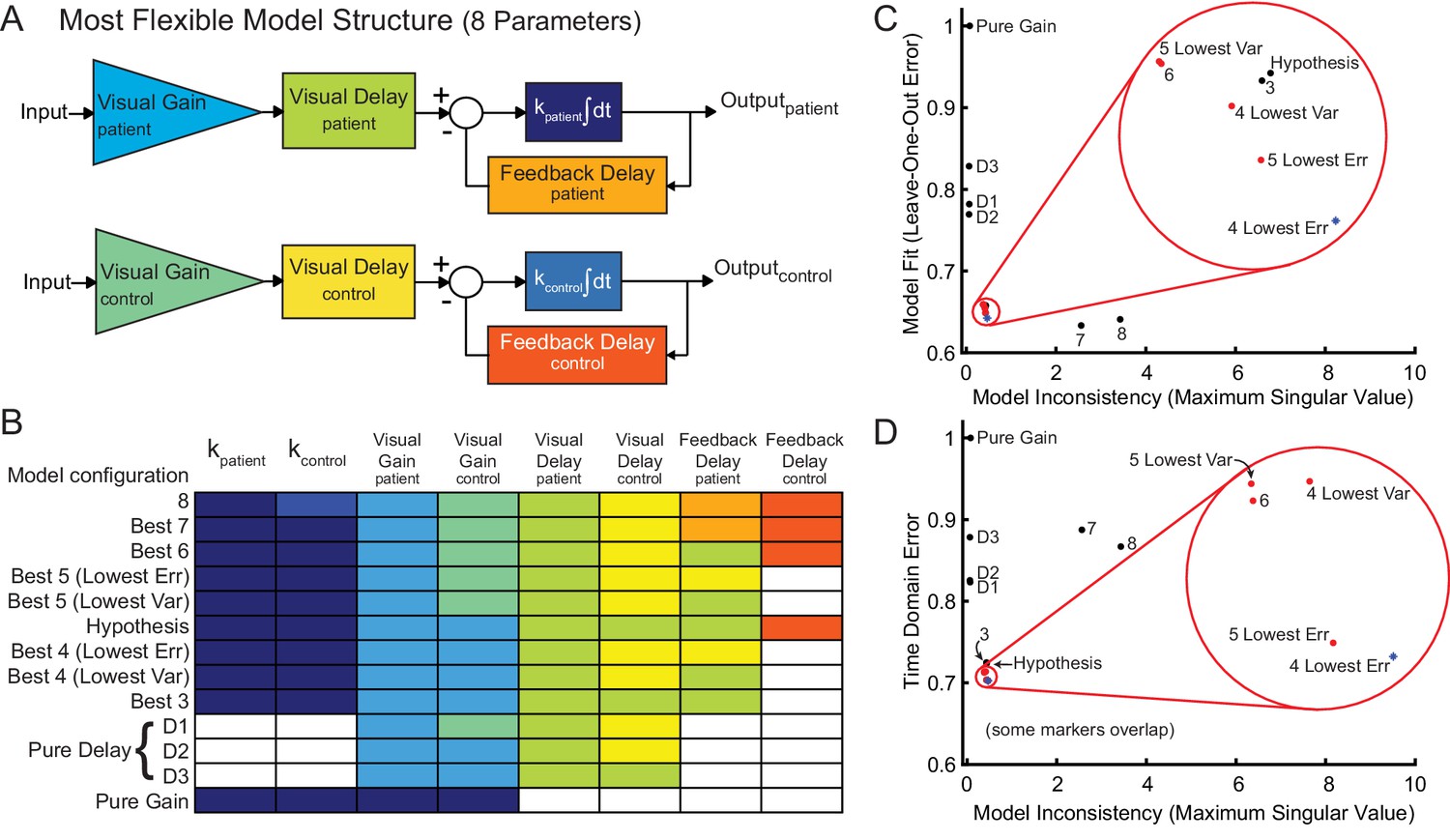
(A) Our modeling framework was based on the McRuer Crossover model (McRuer and Krendel, 1974). This simple model structure lumps the controller and plant as a scaled integrator, and assigns different delays to the measurement of the target from that of self-movement feedback. We hypothesized that the patient and control models would be equivalent except for the magnitude of the feedback delay. The Visual Gain is necessary because, given the complexity and speed of the signal, participants were unable to match the full magnitude of the signal. (B) After our model selection procedure, the Final Model structure was distilled from the top models to capture the general features shared among them. It is similar to our hypothetical model, but with subtle differences: the feedback delay for the controls was determined to be zero instead of equivalent to the proprioceptive delay, the feedback delay for patients was shorter than or equal to the visual delay, and the visual delay for patients was slightly longer than healthy controls. (C) Time domain visualization of subject and model responses for a typical 15 s time window of our experiments. The same visual target trajectory (green) was played to all patients and controls and was used in simulation. Individual time-domain elbow-angle responses (light gray) are shown for the 11 control subjects (top plot) and 11 patients (bottom plot). The average subject responses (orange, solid) match with reasonable accuracy the simulated model responses (orange, dashed). The simulated model structure used here is the modeled named ‘Best 4 (Lowest Err)’ in Figure 4—figure supplement 1B.
Figure 4—figure supplement 1
Model fitting and model selection.
We used sum-of-sine data to fit the parameters of a modified McRuer Crossover model (McRuer and Krendel, 1974). (A) In the most flexible setting, there are a total of eight free parameters, allowing for patients and controls to have completely independent model parameters. (B) In the model fitting and model selection process, we tested all possible variations of the model structure, for a total of 2667 model configurations. For example, some model structures yoke parameters together or eliminate parameters, and some yoke variables together across patient and control models. Each row illustrates an individual model configuration. Variables with the same color within that row are yoked together for that model configuration and white indicates that the specified variable was removed from the model. The table includes the following: the best model structures for all possible numbers of free parameters (Best 1–8); the hypothesized model structure (Hypothesis, shown in C and D); two special pure delay (D1-2) model structures. Best 1 is a pure gain model structure. Best 2 is a pure delay (D3) model structure. The model names are shown in the left column. Lowest Err means lowest Leave-One-Out error. Lowest Var means lowest model inconsistency. (C) Results of model selection procedure in frequency domain for the models in B. The models in red dots and blue asterisk, highlighted in the red circle, provide the best trade-off between minimizing model inconsistency (i.e. minimizing parameter variability and over-fitting) and minimizing error (improving model fit). The top four models are labeled 4 Lowest Err, 4 Lowest Var, 5 Lowest Err and 5 Lowest Var. These top models had nearly equivalent performance according to the model selection criteria. (D) Time domain validation. As in (C), we plotted error versus model inconsistency, but here we used the time-domain error (see Materials and methods). Critically, the time-domain data were not used directly for model fitting, and yet the top models in left bottom corner of the frequency domain are also the top models in the time domain, validating that our frequency-domain model selection process selected the models that were also best in the best time-domain.
Figure 4—figure supplement 2
Frequency responses.
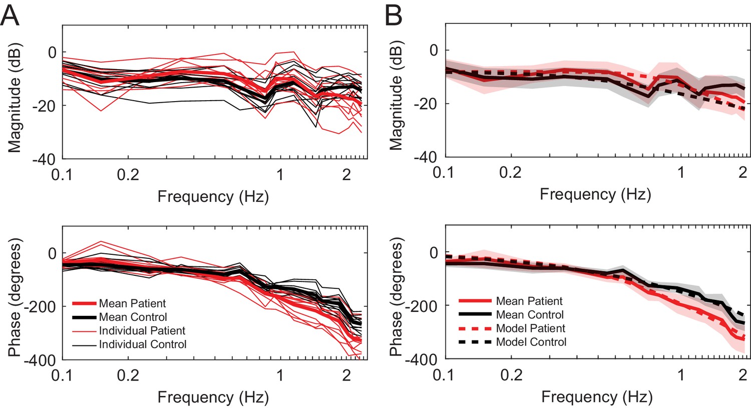
(A) Individual frequency responses for the 11 control subjects (black) and 11 patients (red). It also shows the average responses for controls (black bolded) and patients (red bolded). (B) Mean responses with standard deviation for controls (black bold line with grey shaded region) and patients (red bold line with red shaded region). The simulated model frequency responses (dashed lines) match the actual mean responses well. The frequency responses of the simulated models capture qualitative features, such as the crossing of the response curves between patients and controls both in the magnitude and phase. The simulated model here is Best 4 (Lowest Err).
Figure 5
Patients and controls have categorically different responses to single-sine and sum-of-sine stimuli.
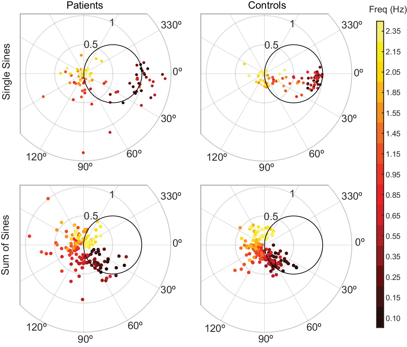
Each data point is the response at a single frequency (magnitude and phase) of a single subject. The patient data in both the single and sum-of-sines conditions are more variable than that of the control subjects. In the single-sines condition, control subjects are able to consistently remain inside the effort/error circle at low frequencies, balancing the tradeoff between effort and error, while patients are not. This result is consistent with previous studies that show patients have impaired prediction.
Figure 6
Phase lags show different patterns between groups.
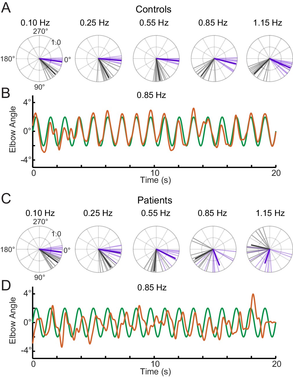
Polar plot representations showing phase lag for the five lowest frequencies common to the single-sine and sum-of-sines conditions. (A) Control group phase lags. Individual subjects are represented as lighter colored unit vectors and the group mean vector is plotted in bold. Purple indicates the single-sine condition and black represents the sum-of-sines condition. Note that only phase lag is represented on the polar plot (gain is not represented). The Control group is able to track the single-sine stimuli with little or no phase lag, but shows phase lags that increase with frequency in the sum-of-sines condition. (B) Example response from a control subject tracking a 0.85 Hz single-sine stimuli. The target sine wave is represented in green and the subject performance in orange. Note that this control could predict the single-sine and track it with little or no phase lag. (C) Cerebellar group phase lags plotted as in A. The Cerebellar patients were able to track the two slowest single-sine stimuli with little phase lag (purple, 0.10 and 0.25 Hz) but then shows increasing phase lags as a function of frequency. Note that 0.10 and 0.25 Hz are extremely slow frequencies that could be followed using only visual feedback control. In the sum-of-sines condition, the cerebellar group shows phase lags that increase with frequency. (D) Example response from a cerebellar subject tracking a 0.85 Hz single-sine stimuli. In contrast to the control subject, this cerebellar patient shows phase lags relative to the target.
Figure 7
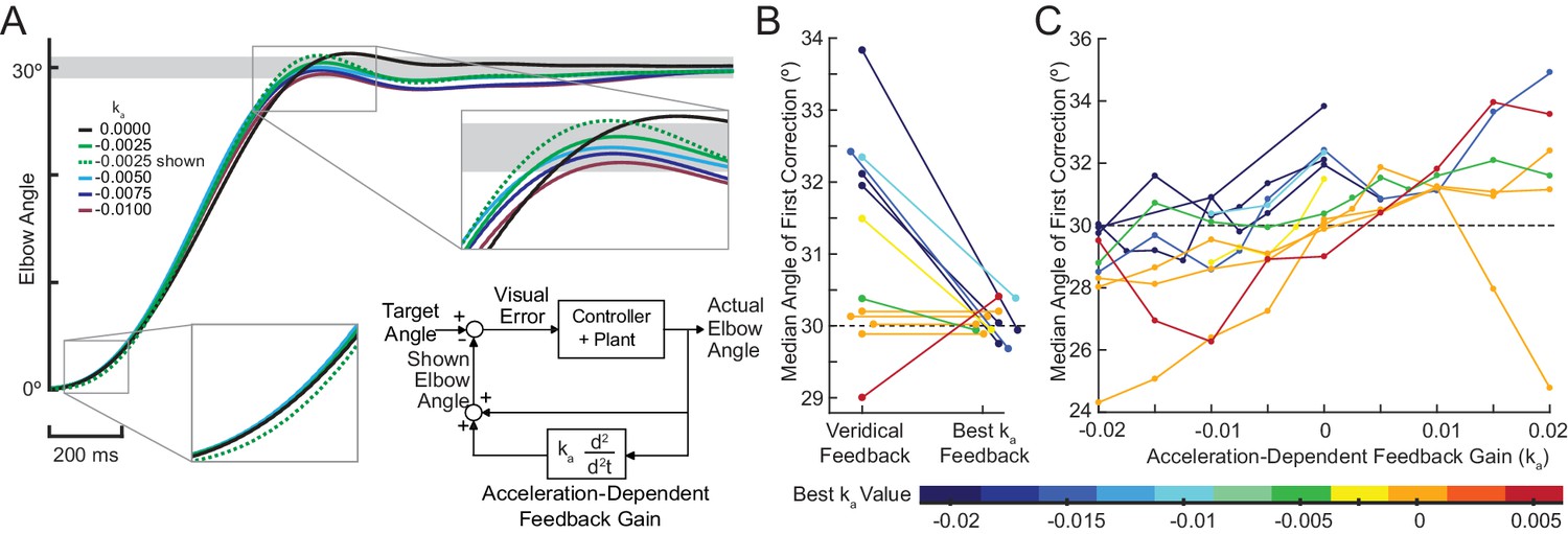
Acceleration-dependent feedback reduces dysmetria.
(A) The trajectories from a single cerebellar patient, moving to the grey target zone. Overshooting or undershooting the grey region is categorized as hypermetric or hypometric, respectively. The solid lines are average trajectories (across trials for a single subject) at a given Acceleration-Dependent Feedback Gain value. A decrease in the angle of first correction (i.e. the peak of the first peak of the elbow angle) is apparent as the Acceleration-Dependent Feedback Gain decreases. The best Acceleration-Dependent Feedback Gain for this subject was determined to be −0.0025, and the resulting movement trajectory is shown as a solid green line. The dashed green line illustrates the trajectory that is displayed to the subject on the screen for the −0.0025 condition. This example also shows that oscillation around the target remains with Acceleration-Dependent Feedback Gain. The block diagram in the lower right shows how the Acceleration-Dependent Feedback Gain was applied to the visual representation of the fingertip position. (B) The reduction in dysmetria exhibited by patients when the best Acceleration-Dependent Feedback Gain was applied. Each line represents a single cerebellar patient. Lines are color coded to indicate the best Acceleration-Dependent Feedback Gain for that subject. (C) Increasing Acceleration-Dependent Feedback Gain causes increased hypermetria. Again, each line represents a single cerebellar patient. At the highest gain values, the visual feedback diverged enough from the fingertip position so that some subjects paused mid-reach, presumably due to the conflicting visual feedback. This yielded the observed drop in median angle of first correction seen in some subjects in the higher gain conditions. This figure shows only the cerebellar patients. Control subject data is shown in Figure 8.
Figure 8
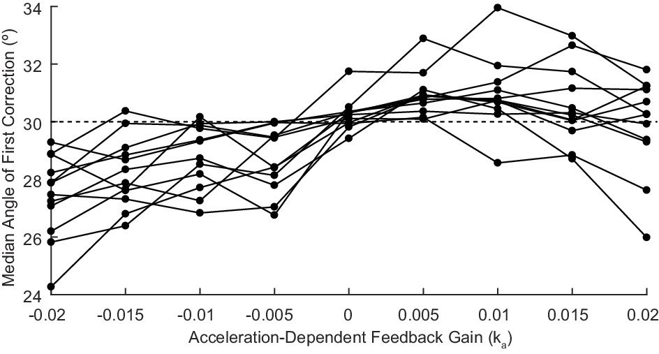
Acceleration-Dependent Feedback also affects single reaches in control subjects.
Control subjects’ median angle of first correction when completing thirty-degree flexion movements. The expected upward trend in median angle of first correction is visible across subjects. At the largest Acceleration-Dependent Feedback Gains, there is a slight drop off in median angle of first correction. At high gain values, the discrepancy between the cursor and the fingertip became more apparent, causing some subjects to pause mid-reach, resulting in a lower median angle of first correction for these high gain conditions.
Figure 9

Our modeling results agree with the theory of the cerebellum as a Smith Predictor.
A basic model for the control system is shown in the top panel. In our experiment, the plant, P, represents the entire mechanical arm system, including the robot exoskeleton arm. A single visual delay block delays the input from both the reference signal and the feedback information. A visual gain scales the amount of the input the subject will attempt to replicate. The brain, illustrated by a dashed box, can be modeled as containing just a controller, C, as shown on the right side. Or, the brain can be modeled as a controller with an accompanying Smith Predictor, as shown on the left side. When these two alternate structures are simplified, we are left with the exact model structures yielded by our previous modeling results.
Author response image 1

Author response image 2
Tables
Table 1
The cerebellar patient population that was tested.
Not all subjects completed all experiments. Some subjects completed the experiments over two visits. Upper Limb ICARS contains the sum of the upper-limb kinetic function elements of the test (ICARS subsections 10–14, out of 20).
| Subject no. | Patient age | Sex | Pathology | Icars | Upper limb ICARS | Experiments |
|---|---|---|---|---|---|---|
| P1 | 44 | M | SCA8 | 62 | 17 | 1,2,3 |
| P2 | 52 | M | ADCAIII | 28 | 8 | 3 |
| P3 | 53 | M | Sporadic | 59 | 19 | 1,2,3 |
| P4 | 55 | F | SCA8 | 41 | 17 | 3 |
| P5 | 55 | M | OPCA | 46 | 14 | 1,2 |
| P6 | 60 | M | MSA-C | 63 | 14 | 1,2,3 |
| P7 | 62 | F | Sporadic | 36 | 16 | 1,2 |
| P8 | 62 | M | SCA6/8 | 62 | 19 | 1,2,3 |
| P9 | 63 | M | SCA6 | 41 | 10 | 3 |
| P10 | 64 | F | SCA6 | 58 | 13 | 1,2 |
| P11 | 64 | M | ADCAIII | 11 | 3 | 1,2,3 |
| P12 | 65 | M | Idiopathic | 34 | 10 | 3 |
| P13 | 66 | F | SCA6 | 41 | 11 | 1,2 |
| P14 | 67 | F | Left cerebellar stroke | 27 | 10 | 1,2,3 |
| P15 | 69 | F | ADCAIII | 52 | 13 | 3 |
| P16 | 72 | F | SCA6 | 49 | 18 | 3 |
| P17 | 78 | M | Sporadic (Vermis Degen.) | 39 | 6 | 1,2 |
Table 2
Model parameters with standard deviation for the top models (Best 5 and Best 4).
Variables with the same color within a row are yoked together for that model configuration. Top models are similar; the feedback delay was smaller than or equal to the visual delay for the patients, and zero for controls, and the patient visual delay was longer than that of the healthy controls.
| Model | kpatient | kcontrol | Visual Gainpatient | Visual Gaincontrol | Visual Delaypatient (ms) | Visual Delaycontrol (ms) | Feedback Delaypatient (ms) | Feedback Delaycontrol (ms) |
|---|---|---|---|---|---|---|---|---|
| Best 5 (Lowest Err) | 2.8 (0.09) | 2.8 (0.09) | 0.38 (0.01) | 0.41 (0.02) | 211 (0.008) | 143 (0.003) | 143 (0.003) | 0 |
| Best 5 (Lowest Var) | 2.6 (0.08) | 2.6 (0.08) | 0.37 (0.01) | 0.42 (0.02) | 183 (0.005) | 147 (0.003) | 183 (0.005) | 0 |
| Best 4 (Lowest Err) | 2.7 (0.10) | 2.7 (0.10) | 0.39 (0.01) | 0.39 (0.01) | 210 (0.007) | 141 (0.003) | 141 (0.003) | 0 |
| Best 4 (Lowest Var) | 2.5 (0.09) | 2.5 (0.09) | 0.40 (0.01) | 0.40 (0.01) | 181 (0.005) | 145 (0.003) | 181 (0.005) | 0 |
Table 3
Hypothesized changes in model parameters under different Feedback Gains.
The table shows how we expect the model parameter values indicated in the bottom two rows (1.35 and 0.65 Feedback Gain) to change (with respect to the value obtained in the veridical Feedback Gain condition, Feedback Gain = 1.0) with changing Feedback Gains. We expect Visual Delay of approximately 140 to 250 ms, and Proprioceptive Delay approximately 110 to 150 ms (Cameron et al., 2014). We also expect Visual Gain to be less than one in the veridical feedback condition because we do not expect the subjects to attempt to replicate the full magnitude of the signal, given that it is a challenging, fast, and unpredictable task.
| Feedback Gain | K | Visual gain | Visual delay (s) | Feedback Delaypatient (s) | Feedback Delaycontrol (s) |
|---|---|---|---|---|---|
| 1.0 | <1 | Visual Delay | Visual Delay | Proprioceptive Delay | |
| 1.35 | Decrease | Increase | Unchanged | Unchanged | Unchanged |
| 0.65 | Increase | Decrease | Unchanged | Unchanged | Unchanged |
Table 4
The model (Best 4 Lowest Err) parameters changed with different applied Feedback Gains in a manner consistent with our prediction.
| Feedback Gain | kpatient | kcontrol | Visual Gainpatient | Visual Gaincontrol | Visual Delaypatient (ms) | Visual Delaycontrol (ms) | Feedback Delaypatient (ms) | Feedback Delaycontrol (ms) |
|---|---|---|---|---|---|---|---|---|
| 1 | 2.7 | 2.7 | 0.39 | 0.39 | 210 | 141 | 141 | 0 |
| 1.35 | 2.2 | 2.2 | 0.44 | 0.44 | 209 | 140 | 140 | 0 |
| 0.65 | 3.6 | 3.6 | 0.33 | 0.33 | 210 | 144 | 144 | 0 |
Additional files
Download links
A two-part list of links to download the article, or parts of the article, in various formats.
Downloads (link to download the article as PDF)
Open citations (links to open the citations from this article in various online reference manager services)
Cite this article (links to download the citations from this article in formats compatible with various reference manager tools)
Cerebellar patients have intact feedback control that can be leveraged to improve reaching
eLife 9:e53246.
https://doi.org/10.7554/eLife.53246


