Top-down machine learning approach for high-throughput single-molecule analysis
- Department of Neuroscience, University of Wisconsin-Madison, United States
- Department of Chemistry, University of Wisconsin-Madison, United States
- Department of Neuroscience, University of Texas at Austin, United States
- Department of Biomolecular Chemistry University of Wisconsin-Madison, United States
Figures
Figure 1 with 1 supplement
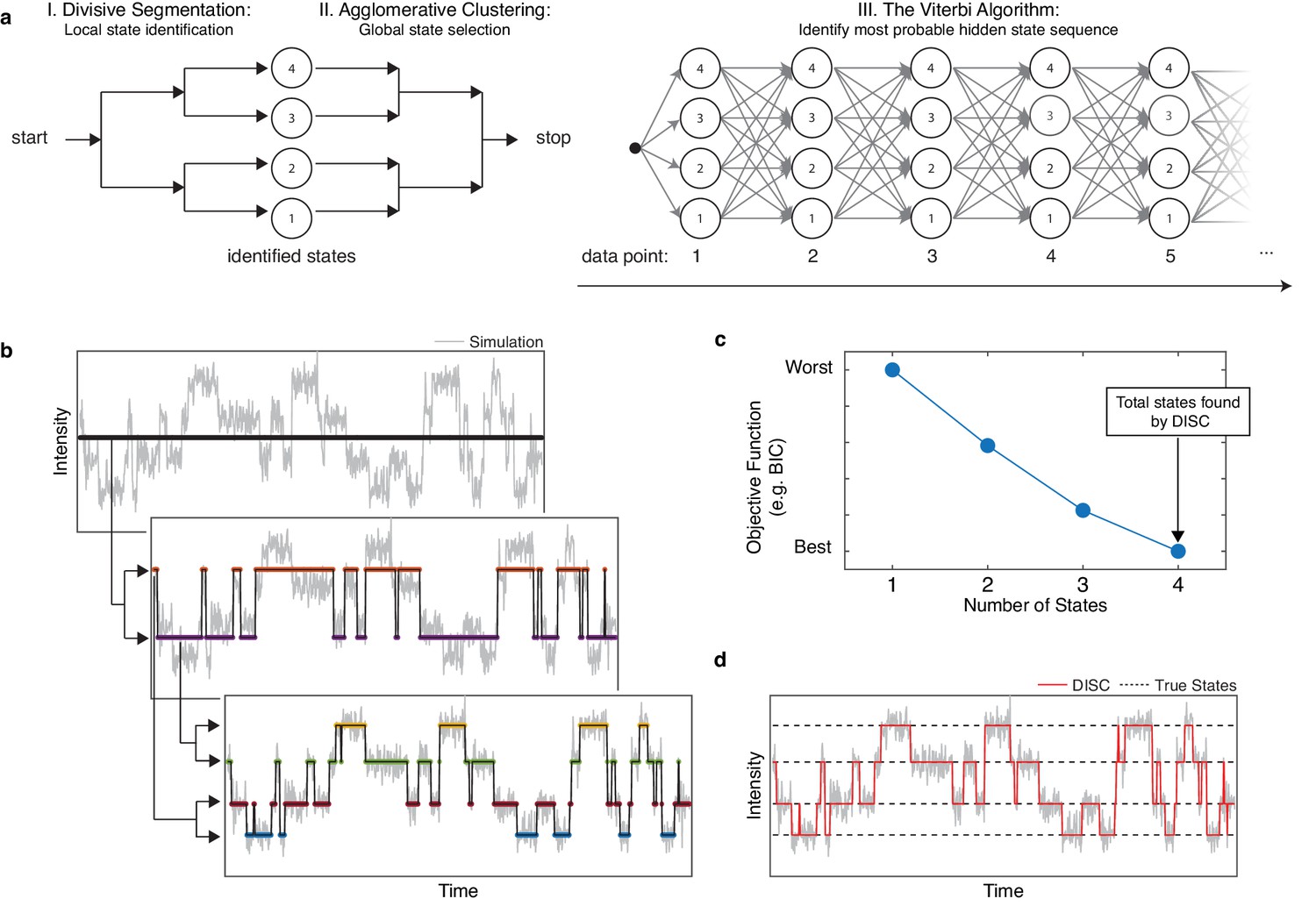
Overview of DISC.
(a) The major steps of the DISC algorithm combining unsupervised statistical learning with the Viterbi algorithm. (b) Stepwise discovery of states locally through divisive segmentation on a simulated trajectory. (c) HAC iteratively groups identified states to minimize an objective function for the fit of the whole trajectory to avoid overfitting. (d) The Viterbi algorithm is applied to identify the most probable hidden state sequence. The final fit by DISC (red) is overlaid against the true states in the simulation (dashed).
-
Figure 1—source data 1
Plotted simulated data with DISC fit.
- https://cdn.elifesciences.org/articles/53357/elife-53357-fig1-data1-v2.xlsx
Figure 1—figure supplement 1
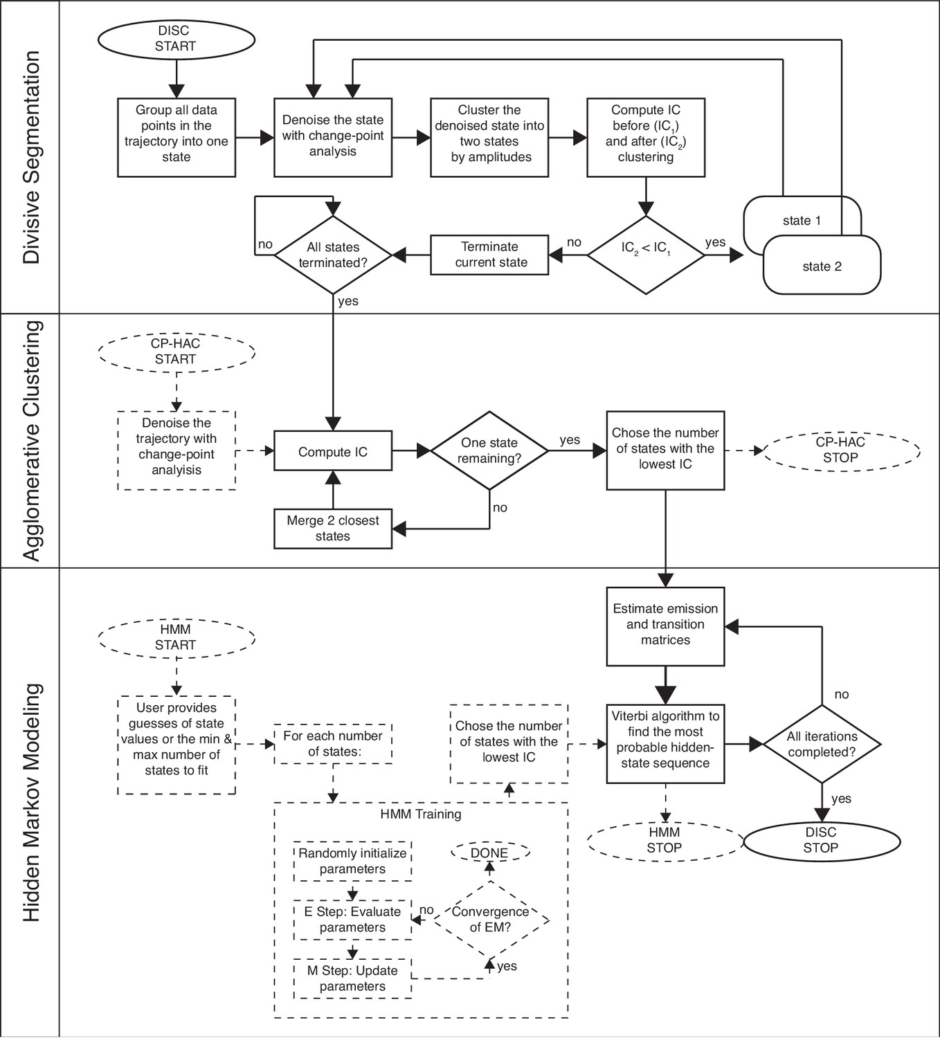
Workflow of DISC.
Solid lines indicate the path DISC takes through divisive segmentation, hierarchical agglomerative clustering, and the Viterbi algorithm. IC = information criterion. General CP-HAC and HMM approaches are shown for comparison. Dotted lines indicate steps that do not overlap with DISC. Ovals indicate start/stop; rectangles indicate a process or computation; diamonds represent decisions. Note, most current uses of HMMs involve a single user-defined number of states.
Figure 2 with 1 supplement
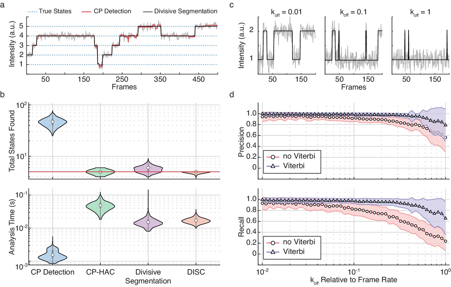
Refinement of divisive segmentation.
(a) Example trajectory simulated with five states (blue) at a SNR = 5 overlaid with fits obtained from change-point detection (red) and divisive segmentation (black). (b) Violin plots showing the number of identified states (top) and analysis time (bottom) of each algorithm across 500 simulated trajectories featuring five true states (red line). (c) Example simulations of a two-state system with a kon = 0.02 frames−1 and varying koff. (d) Precision (top) and recall (bottom) values obtained with CP detection (no Viterbi) and Viterbi refinement obtained across 100 trajectories per koff (mean ± s.d.).
-
Figure 2—source data 1
Simulated data of varying dynamics.
- https://cdn.elifesciences.org/articles/53357/elife-53357-fig2-data1-v2.xlsx
Figure 2—figure supplement 1
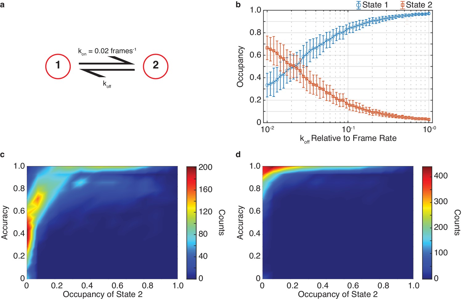
The effect of state occupancy on DISC.
(a) Simulated kinetic scheme of Figure 2 featuring two states with a constant kon (kon = 0.02 frames−1) and varying koff. (b) Occupancy of state 1 (blue circles) and state 2 (orange squares) for different simulated koff values (mean ± s.d.). (c, d) Density plot of idealization accuracy per trajectory vs the occupancy of state two across all simulations (N = 5000) for results obtained without (c) and with Viterbi refinement (d).
Figure 3 with 3 supplements

Standardizing performance.
(a) Average accuracy (top), precision (middle) and recall values (bottom) computed for DISC, STaSI, and vbFRET across 100 trajectories at the specified signal to noise and number of states (Materials and methods). (b) Example simulated trajectory with four true states (red) fit and added Gaussian noise (grey) to SNR = 6 overlaid with fits (black) from DISC (top), STaSI (middle), or vbFRET (bottom).
-
Figure 3—source data 1
Algorithm results of CNBD simulations.
- https://cdn.elifesciences.org/articles/53357/elife-53357-fig3-data1-v2.xlsx
Figure 3—figure supplement 1
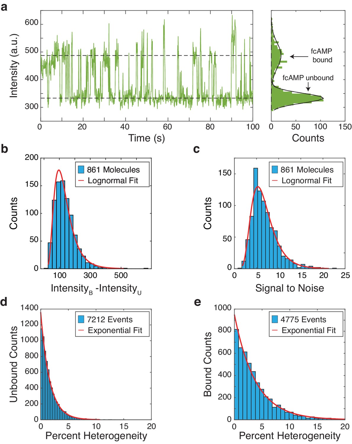
Characterization of fcAMP binding to monomeric CNBDs in ZMWs.
(a) Representative trajectory of a fcAMP binding to a monomeric CNBD in a ZMW (b) Intensity difference of bound (B) and unbound (U) states per trajectory with a log-normal fit (µ = 4.79, σ = 0.47, N = 861) (c) Signal-to-noise per trajectory with a log-normal fit (µ = 1.84, σ = 0.41, N = 861) (c). Quantification of unbound (d) and bound (e) event heterogeneity overlaid with exponential fits (unbound µ = 1.62, bound µ = 3.81).
Figure 3—figure supplement 2
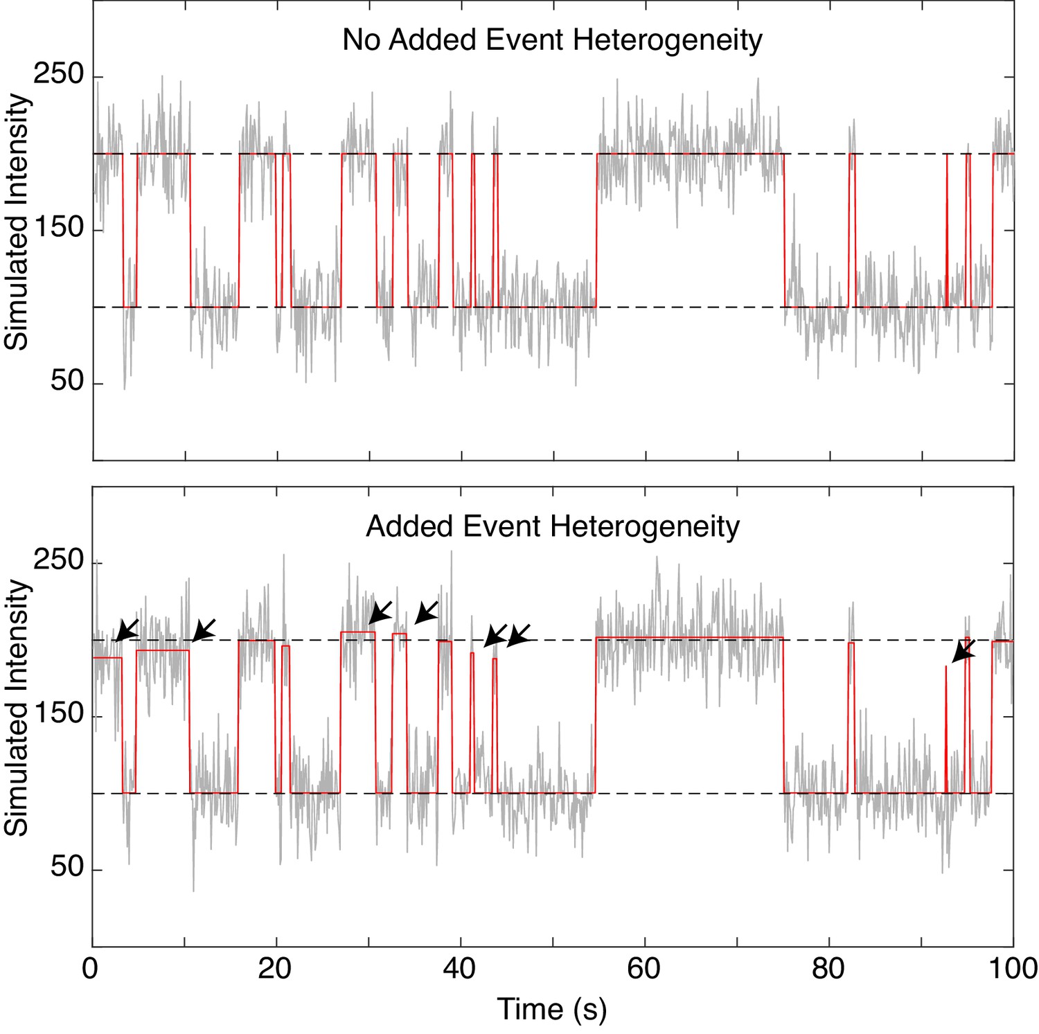
Simulation with heterogenous fcAMP emission.
Representative SM simulation of a two-state system both without (top) and without (bottom) heterogeneous emission of fcAMP upon binding. Plots show simulated trajectory (red) overlaid with the addition of Gaussian noise (grey) and the average intensity value of each state (dashed black). Arrows indicate events where the heterogeneous intensities show prominent deviations away from the mean state value.
Figure 3—figure supplement 3
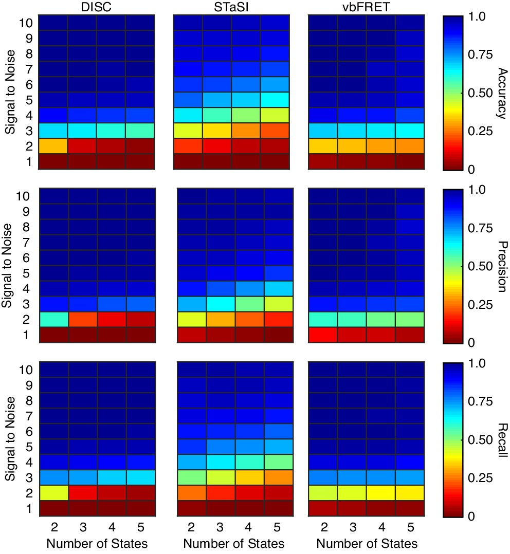
Algorithm performance on simulations without heterogenous fcAMP emission.
Recreation of simulations from Figure 3 of the main text without the inclusion of heterogenous intensities per binding event. Each value is the average accuracy (top), precision (middle), and recall (bottom) across 100 trajectories 200-second-long trajectories collected at 10 Hz at the indicated SNR and number of states (Materials and methods).
Figure 4 with 1 supplement

The effect of trajectory length on DISC performance.
(a) Computational time (mean ± s.d.) of each algorithm for analyzing single trajectories of varying lengths. The test was performed with an Intel Xeon, 3.50 GHz processor running MATLAB 2017a. (b) Accuracy (mean ± s.d., N = 5000) of DISC for simulated trajectories of a two-state model with varying SNR and total number of data points.
-
Figure 4—source data 1
Algorithm results across varying trajectory length.
- https://cdn.elifesciences.org/articles/53357/elife-53357-fig4-data1-v2.xlsx
Figure 4—figure supplement 1
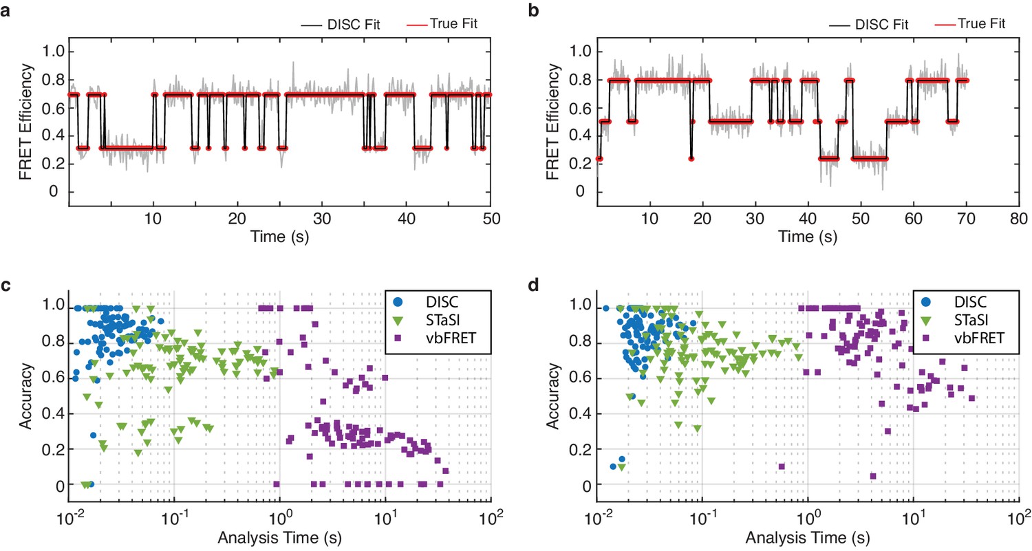
Algorithm performance on simulated smFRET data.
(a, b) Representative fits of simulated smFRET data with 2 (a) or 3 (b) states (red) overlaid with the idealized fits from DISC (black). (c, d) Scatter plot of accuracy vs analysis time of 100 simulated smFRET trajectories featuring 2 (c) or 3 (d) states analyzed by DISC (blue circles), STaSI (green triangles) and vbFRET (purple squares).
Figure 5 with 5 supplements
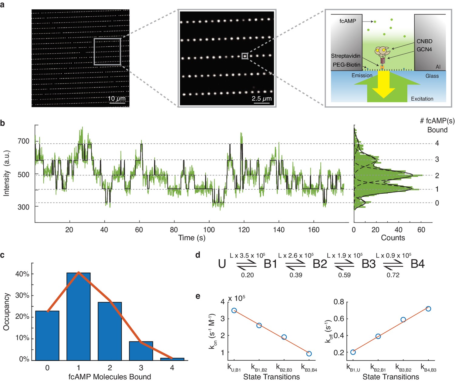
DISC analysis of HCN CNBDs.
(a) Representative ZMW arrays for observing fcAMP binding to tethered tetrameric CNBD. (b) Representative time series of 1 µM fcAMP binding to tetrameric CNBD fit with DISC with up to four fcAMP molecules binding simultaneously. (c) Observed distribution of fcAMP occupancy fit with a binomial distribution (orange). (d) Sequential model of four binding steps and one unbound state with globally optimized rate constants. The rate constants are given as s−1 or s−1M−1 where L is the ligand concentration in M. (e) Linear regression of rate constants kon (m = −8.5×10⁴ s−1M−1, b = 4.35×10⁵ s−1M−1, R2 = 0.99) and koff (m = 0.18 s−1, b = 0.035 s−1, R2 = 0.99) for each sequential state.
-
Figure 5—source data 1
Plotted data and fits of tetrameric CNBD dynamics.
- https://cdn.elifesciences.org/articles/53357/elife-53357-fig5-data1-v2.xlsx
Figure 5—figure supplement 1
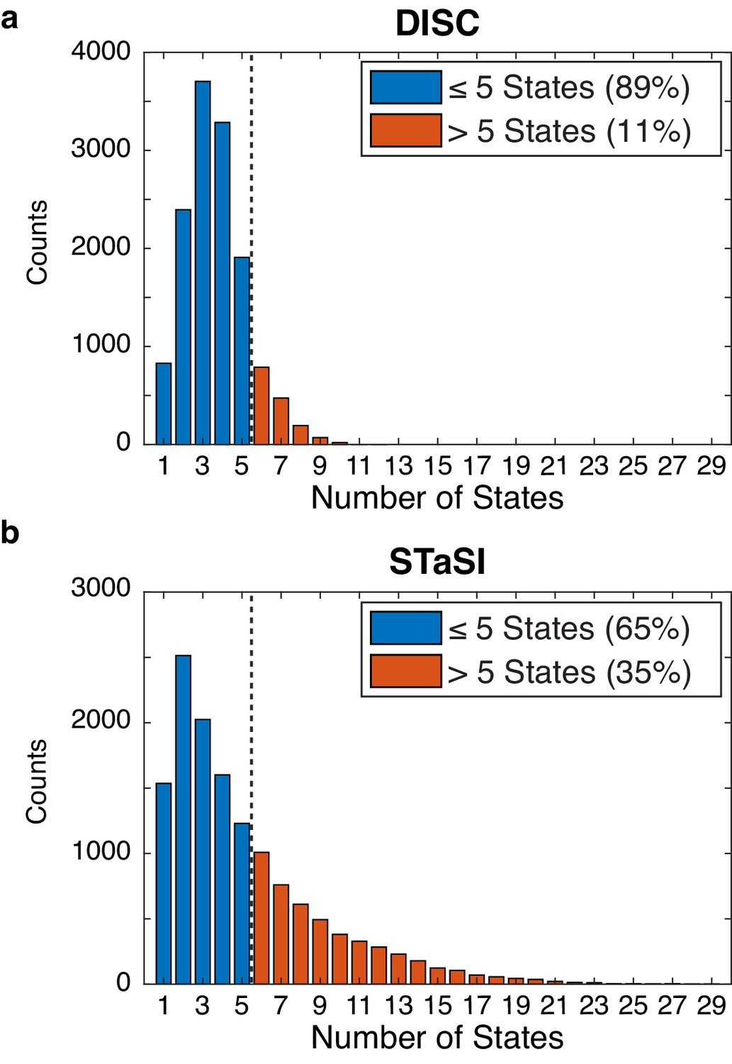
Tetrameric CNBD analysis by DISC and STaSI.
Initial number of states found by DISC (a) and STaSI (b) when run on the tetrameric CNBD data set across 13,670 trajectories prior to trace selection (Materials and methods). The expected distribution is between 1 and 5 states per trajectory to account for empty ZMWs and fully occupied tetrameric CNBDs (four fcAMP bound states plus one unbound state). This analysis was not repeated using vbFRET as we estimated the process would take weeks to complete.
Figure 5—figure supplement 2
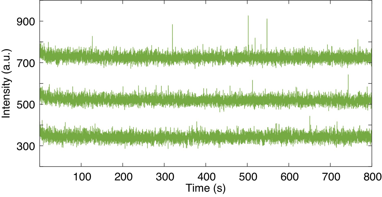
Non-specific fcAMP binding in ZMWs.
Representative trajectories of unoccupied ZMWs in the presence of 1 µM fcAMP. Trajectories are offset by 200 arbitrary units (a.u.) for visualization.
Figure 5—figure supplement 3
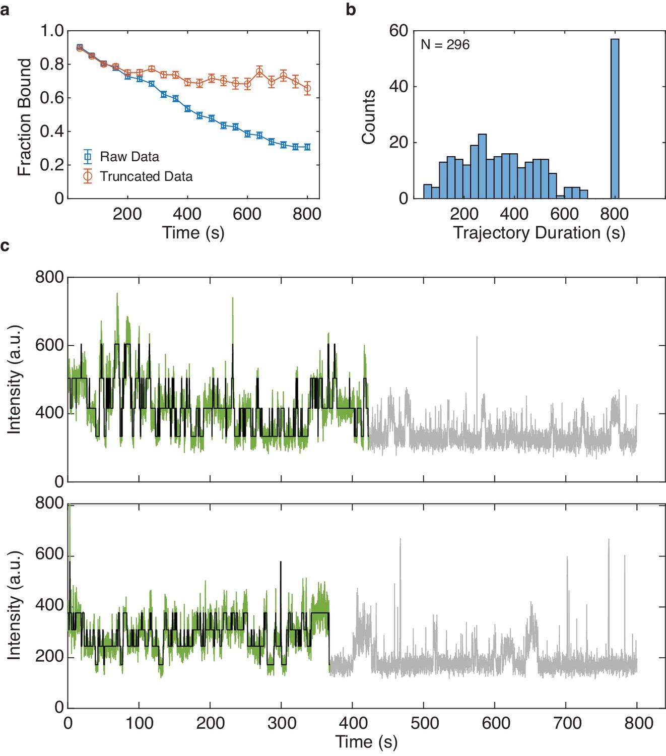
Asynchronous decay of tetrameric CNBD activity over excitation time.
(a) Average fraction bound of each molecule over time (binned every 40 s) before and after trajectory truncation (mean ± s.e.m., see Materials and methods). (b) Distribution of trajectory durations following truncation (N = 296). Each trajectory was initially 800 s. (c) Representative trajectories showing the truncated data kept for analysis (green) with idealized fit by DISC (black) and the discarded frames (grey).
Figure 5—figure supplement 4
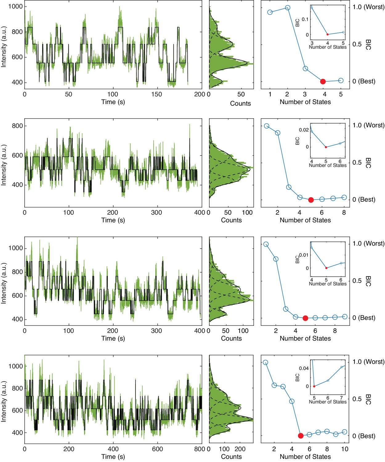
Example trajectories of 1 µM fcAMP binding to tetrameric CNBDs in ZMWs.
Representative trajectories featuring up to 3 or four bound fcAMP molecules analyzed by DISC (left) with distribution fits (middle) and BIC curves for optimal state selection (right). Inset shows a zoomed portion of BIC curve to highlight the minimum BIC value identified. The lowest BIC value is indicated in red which corresponds to the final number of states fit to the trajectory. Each BIC plot may feature a different number of total possible states owning to the trajectory-by-trajectory results from divisive segmentation.
Figure 5—figure supplement 5
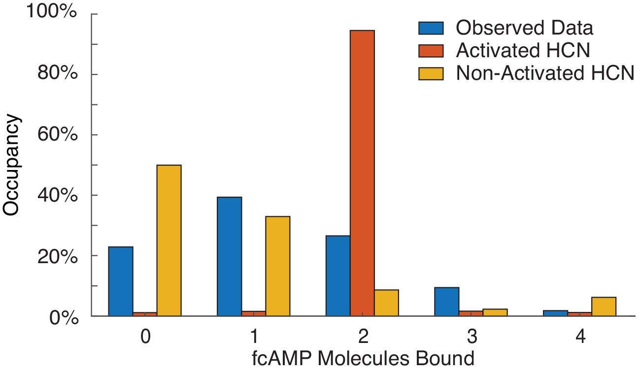
Model comparison of HCN CNBDs.
Comparison of obtained state-occupancy distribution from single-molecule experiments with expected values from activated and non-activated HCN channel models.
Tables
Key resources table
| Reagent type (species) or resource | Designation | Source or reference | Identifiers | Additional information |
|---|---|---|---|---|
| Biological sample | GCN4pLI-HCN2 tetramer | DOI: 10.7554/eLife.20797 | ||
| Chemical compound, drug | Protocatechuate 3,4-Dioxygenase | Millipore-Sigma | cas no. 9029-47-4 | from Pseudomonas sp. |
| Chemical compound, drug | 3,4-Dihydroxybenzoic acid | Millipore-Sigma | cas no. 99-50-3 | Protocatechuic Acid |
| Chemical compound, drug | (±)-6-Hydroxy-2,5,7,8-tetramethylchromane-2-carboxylic acid | Millipore-Sigma | cas no. 53188-07-1 | Trolox |
| Chemical compound, drug | 8-[DY-547]-AET-cAMP | BIOLOG | Cat. No.: D 109 | DOI:10.1016/j.neuron.2010.05.022 |
| Software, algorithm | MATLAB | MathWorks | RID:SCR_001622 | |
| Software, algorithm | QuB | DOI: 10.1142/1793048013300053 | https://qub.mandelics.com/ | |
| Software, algorithm | DISC | This work | https://github.com/ChandaLab/DISC | |
| Software, algorithm | vbFRET | DOI: 10.1016/j.bpj.2009.09.031 | http://vbfret.sourceforge.net/ | |
| Software, algorithm | STaSI | DOI: 10.1021/jz501435p | https://github.com/LandesLab/STaSI | |
| Other | Zero-Mode Waveguide | Pacific Biosciences | Non-Commercial Zero-Mode Waveguides (Astro Chips) |
Additional files
Download links
A two-part list of links to download the article, or parts of the article, in various formats.
Downloads (link to download the article as PDF)
Open citations (links to open the citations from this article in various online reference manager services)
Cite this article (links to download the citations from this article in formats compatible with various reference manager tools)
Top-down machine learning approach for high-throughput single-molecule analysis
eLife 9:e53357.
https://doi.org/10.7554/eLife.53357


