NeuroQuery, comprehensive meta-analysis of human brain mapping
- Inria, CEA, Université Paris-Saclay, France
- Stanford University, United States
- Inria, France
- University of Texas at Austin, United States
- Télécom Paris University, France
- Montréal Neurological Institute, McGill University, Canada
Figures
Figure 1
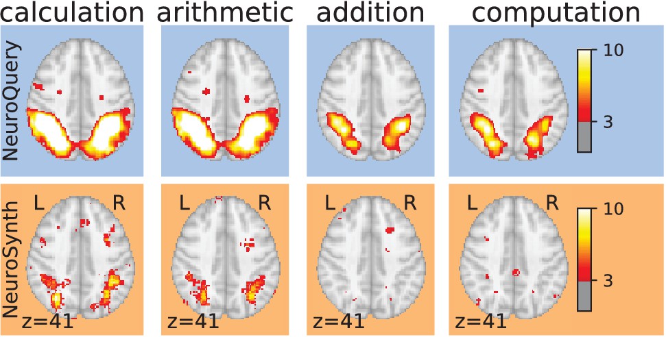
Taming query variability Maps obtained for a few words related to mental arithmetic.
By correctly capturing the fact that these words are related, NeuroQuery can use its map for easier words like ‘calculation’ and ‘arithmetic’ to encode terms like ‘computation’ and ‘addition’ that are difficult for meta-analysis.
Figure 2
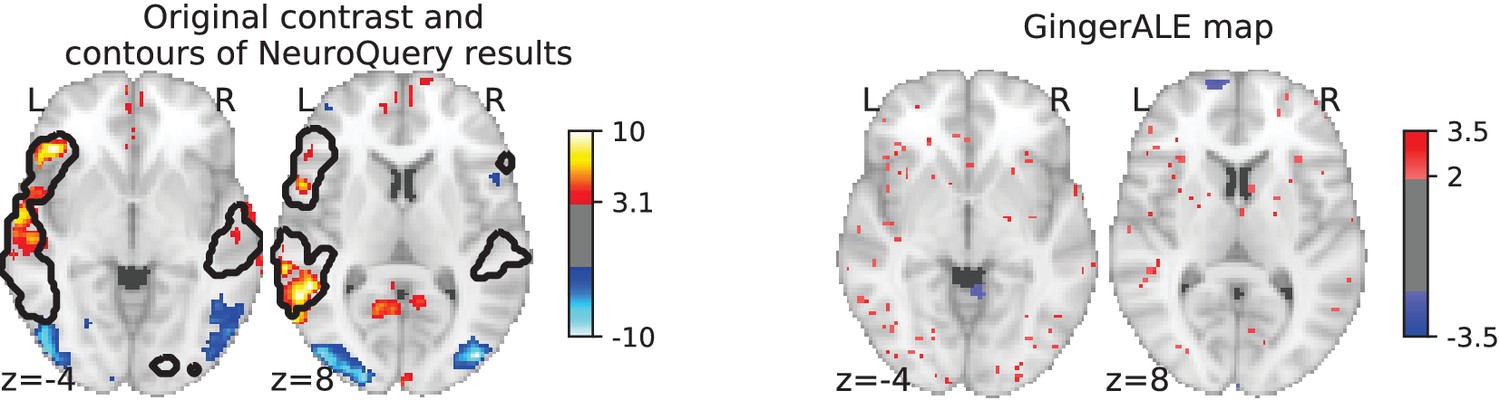
Illustration: studying the contrast ‘Read pseudo words vs. consonant strings’.
Left: Group-level map from the IBC dataset for the contrast ‘Read pseudo-words vs. consonant strings’ and contour of NeuroQuery map obtained from this query. The NeuroQuery map was obtained directly from the contrast description in the dataset’s documentation, without needing to manually select studies for the meta-analysis nor convert this description to a string pattern usable by existing automatic meta-analysis tools. The map from which the contour is drawn, as well as a NeuroQuery map for the page-long description of the RSVP language task, are shown in Section 'Example Meta-analysis results for the RSVP language task from the IBC dataset', in Section 'Example Meta-analysis results for the RSVP language task from the IBC dataset' c and Section 'Example Meta-analysis results for the RSVP language task from the IBC dataset'd respectively. Right: ALE map for 29 studies that contain all terms from the IBC contrast description. The map was obtained with the GingerALE tool (Eickhoff et al., 2009). With only 29 matching studies, ALE lacks statistical power for this contrast description.
Figure 3
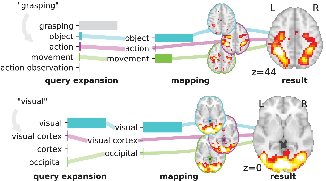
Overview of the NeuroQuery model: two examples of how association maps are constructed for the terms ‘grasping’ and ‘visual’.
The query is expanded by adding weights to related terms. The resulting vector is projected on the subspace spanned by the smaller vocabulary selected during supervised feature selection. Those well-encoded terms are shown in color. Finally, it is mapped onto the brain space through the regression model. When a word (e.g., ‘visual’) has a strong association with brain activity and is selected as a regressor, the smoothing has limited effect. Details: the first bar plot shows the semantic similarities of neighboring terms with the query. It represents the smoothed TFIDF vector. Terms that are not used as features for the supervised regression are shown in gray. The second bar plot shows the similarities of selected terms, rescaled by the norms of the corresponding regression coefficient maps. It represents the relative contribution of each term in the final prediction. The coefficient maps associated with individual terms are shown next to the bar plot. These maps are combined linearly to produce the prediction shown on the right.
Figure 4
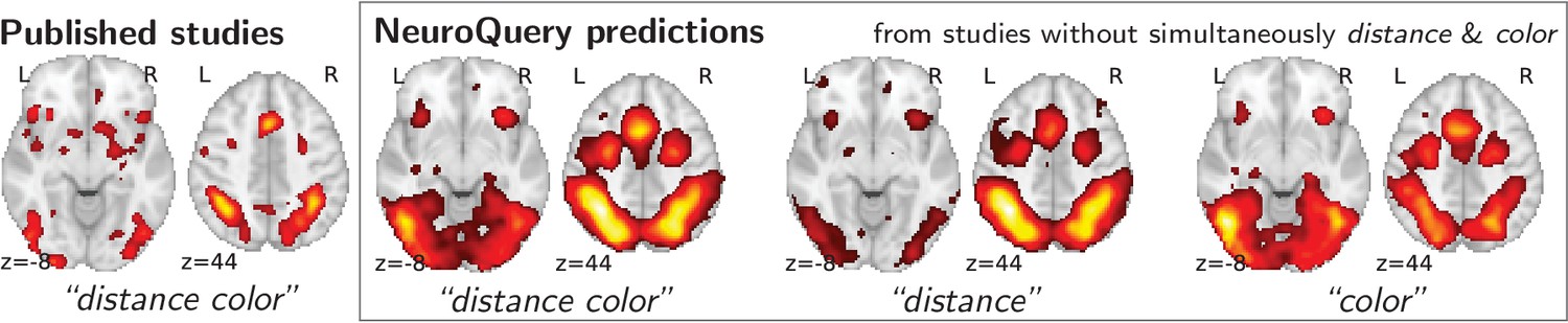
Mapping an unseen combination of terms.
Left The difference in the spatial distribution of findings reported in studies that contains both ‘distance’ and ‘color’ (), and the rest of the studies. – Right Predictions of a NeuroQuery model fitted on the studies that do not contain simultaneously both terms ‘distance’ and ‘color’.
Figure 5
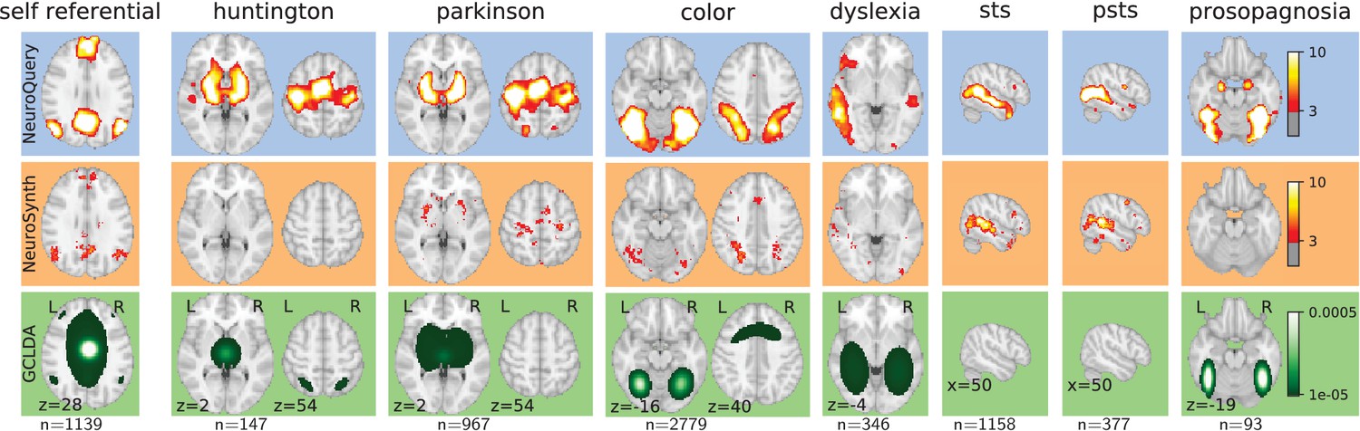
Examples of maps obtained for a given term, compared across different large-scale meta-analysis frameworks.
‘GCLDA’ has low spatial resolution and produces inaccurate maps for many terms. For relatively straightforward terms like ‘psts’ (posterior superior temporal sulcus), NeuroSynth and NeuroQuery give consistent results. For terms that are more rare or difficult to map like ‘dyslexia’, only NeuroQuery generates usable brain maps.
Figure 6
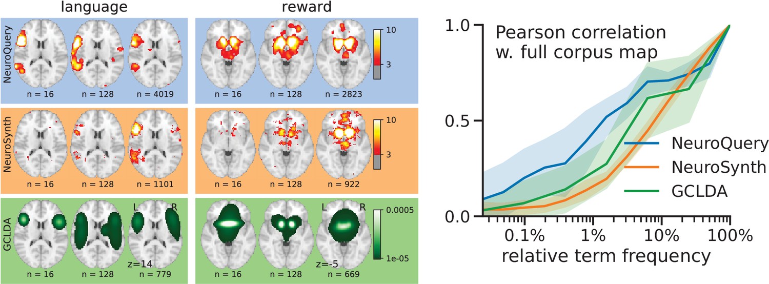
Learning good maps from few studies.
left: maps obtained from subsampled corpora, in which the encoded word appears in 16 and 128 documents, and from the full corpus. NeuroQuery needs less examples to learn a sensible brain map. NeuroSynth maps correspond to NeuroSynth’s Z scores for the ‘association test’ from neurosynth.org. NeuroSynth’s ‘posterior probability’ maps for these terms for the full corpus are shown in Figure 19. Each tool is trained on its own dataset, which is why the full-corpus occurrence counts differ. right: convergence of maps toward their value for the full corpus, as the number of occurrences increases. Averaged over 13 words: ‘language’, ‘auditory’, ‘emotional’, ‘hand’, ‘face’, ‘default mode’, ‘putamen’, ‘hippocampus’, ‘reward’, ‘spatial’, ‘amygdala’, ‘sentence’, ‘memory’. On average, NeuroQuery is closer to the full-corpus map. This confirms quantitatively what we observe for the two examples ‘language’ and ‘reward’ on the left. Note that here convergence is only measured with respect to the model’s own behavior on the full corpus, hence a high value does not indicate necessarily a good face validity of the maps with respect to neuroscience knowledge. The solid line represents the mean across the 13 words and the error bands represent a 95% confidence interval based on 1 000 bootstrap repetitions.
Figure 7
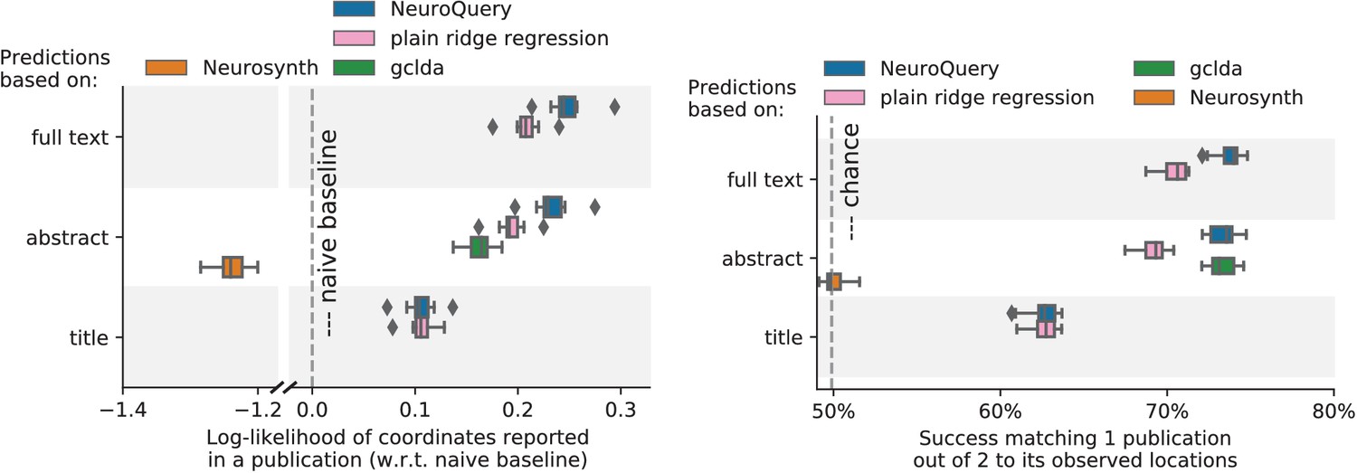
Explaining coordinates reported in unseen studies.
Left: log-likelihood for coordinates reported in test articles, relative to the log-likelihood of a naive baseline that predicts the average density of the training set. NeuroQuery outperforms GCLDA, NeuroSynth, and a ridge regression baseline. Note that NeuroSynth is not designed to make encoding predictions for full documents, which is why it does not perform well on this task. – Right: how often the predicted map is closer to the true coordinates than to the coordinates for another article in the test set (Mitchell et al., 2008). The boxes represent the first, second and third quartiles of scores across 16 cross-validation folds. Whiskers represent the rest of the distribution, except for outliers, defined as points beyond 1.5 times the IQR past the low and high quartiles, and represented with diamond fliers.
Figure 8
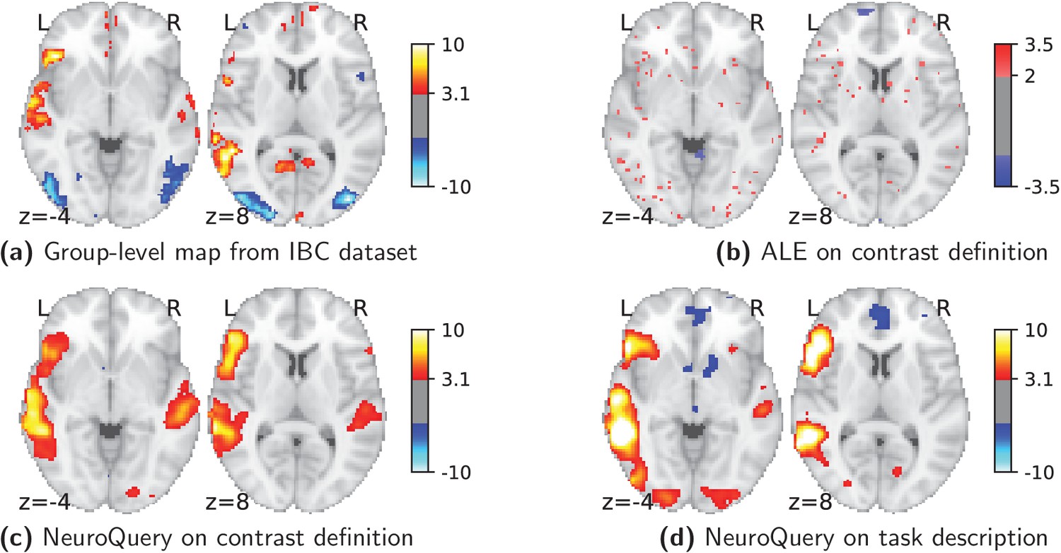
Using meta-analysis to interpret fMRI maps.
Example of the ‘Read pseudo-words vs. consonant strings’ contrast, derived from the RSVP language task in the IBC dataset. (a): the group-level map obtained from the actual fMRI data from IBC. (b): ALE map using the 29 studies in our corpus that contain all five terms from the contrast name. (c): NeuroQuery map obtained from the contrast name. (d): NeuroQuery map obtained from the page-long RSVP task description in the IBC dataset documentation: https://project.inria.fr/IBC/files/2019/03/documentation.pdf.
Figure 9
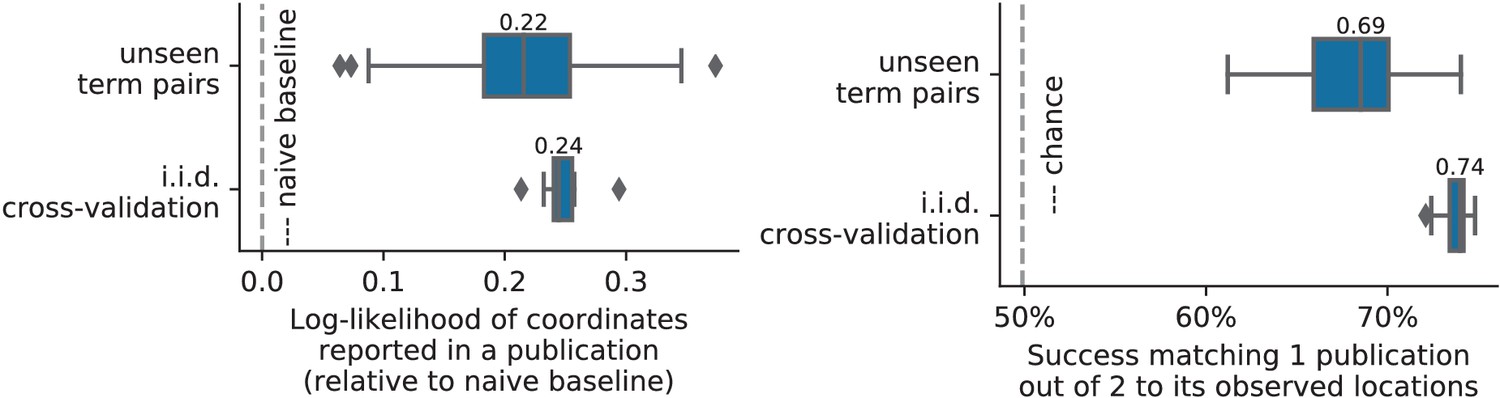
Quantitative evaluations on unseen pairs.
A quantitative comparison of prediction on random unseen studies (i.i.d.cross-validation) to prediction on studies containing pairs of terms never seen before, using the two measures of predictions performance (as visible on Figure 7 for standard cross-validation).
Figure 10
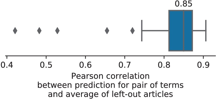
Consistency between prediction of unseen pairs and meta-analysis.
The Pearson correlation between the map predicted by NeuroQuery on a pair of unseen terms and the average density of locations reported on the studies containing this pair of terms (hence excluded from the training set of NeuroQuery).
Figure 11
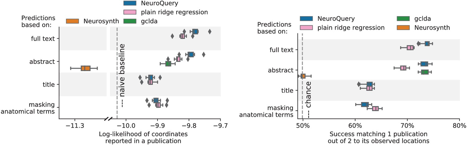
Explaining coordinates reported in unseen studies.
left: log-likelihood of reported coordinates in test articles. right: how often the predicted map is closer to the true coordinates than to the coordinates for another article in the test set [mitchell2008predicting, ]. The boxes represent the first, second and third quartiles of scores across 16 cross-validation folds. Whiskers represent the rest of the distribution, except for outliers, defined as points beyond 1.5 times the IQR past the low and high quartiles, and represented with diamond fliers.
Figure 12

Taming arbitrary query variability Maps obtained for a few words related to mental arithmetic.
By correctly capturing the fact that these words are related, NeuroQuery can use its map for easier words like ‘calculation’ and ‘arithmetic’ to encode terms like ‘computation’ and ‘addition’ that are difficult for meta-analysis.
Figure 13
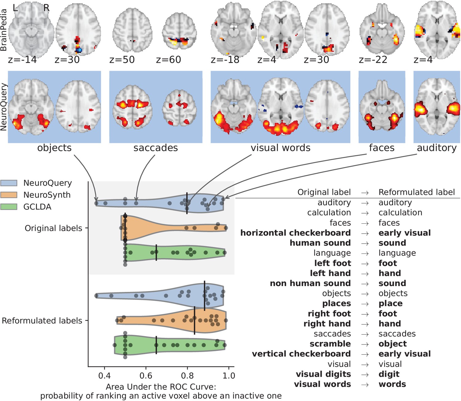
Comparison of CBMA maps with IBMA maps from the BrainPedia study.
We use labelled and thresholded maps resulting from a manual IBMA. The labels are fed to NeuroQuery, NeuroSynth and GCLDA and their results are compared to the reference by measuring the Area under the ROC Curve. The black vertical bars show the median. When using the original BrainPedia labels, NeuroQuery performs relatively well but NeuroSynth fails to recognize most labels. When reformulating the labels, that is replacing them with similar terms from NeuroSynth’s vocabulary, both NeuroSynth and NeuroQuery match the manual IBMA reference for most terms. On the top, we show the BrainPedia map (first row) and NeuroQuery prediction (second row) for the quartiles of the AUC obtained by NeuroQuery on the original labels. A lower AUC for some concepts can sometimes be explained by a more noisy BrainPedia reference map.
Figure 14
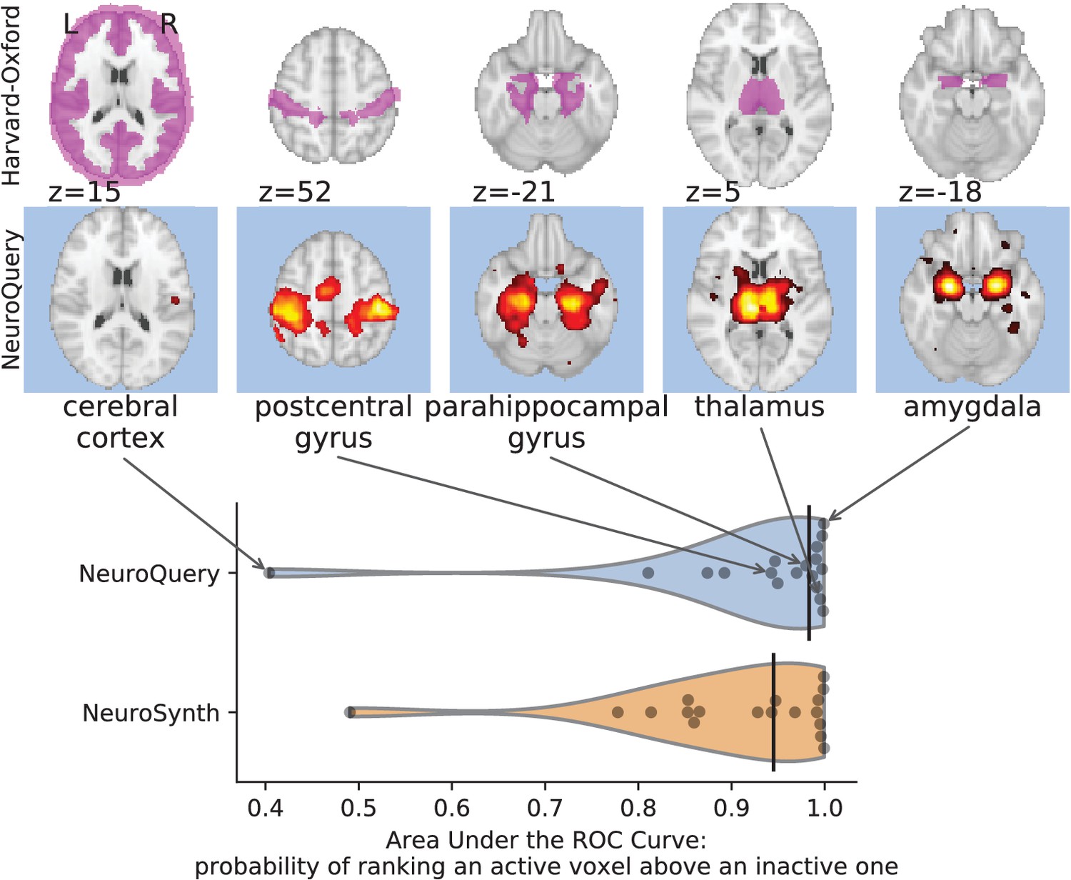
Comparison of predictions with regions of the Harvard-Oxford anatomical atlas.
Labels of the Harvard-Oxford anatomical atlas present in NeuroSynth’s vocabulary are fed to NeuroSynth and NeuroQuery. The meta-analytic maps are compared to the manually segmented reference by measuring the Area Under the ROC Curve. The black vertical bars show the median. Both NeuroSynth and NeuroQuery achieve a median AUC above 0.9. On the top, we show the atlas region (first row) and NeuroQuery prediction (second row) for the quartiles of the NeuroQuery AUC scores.
Figure 15
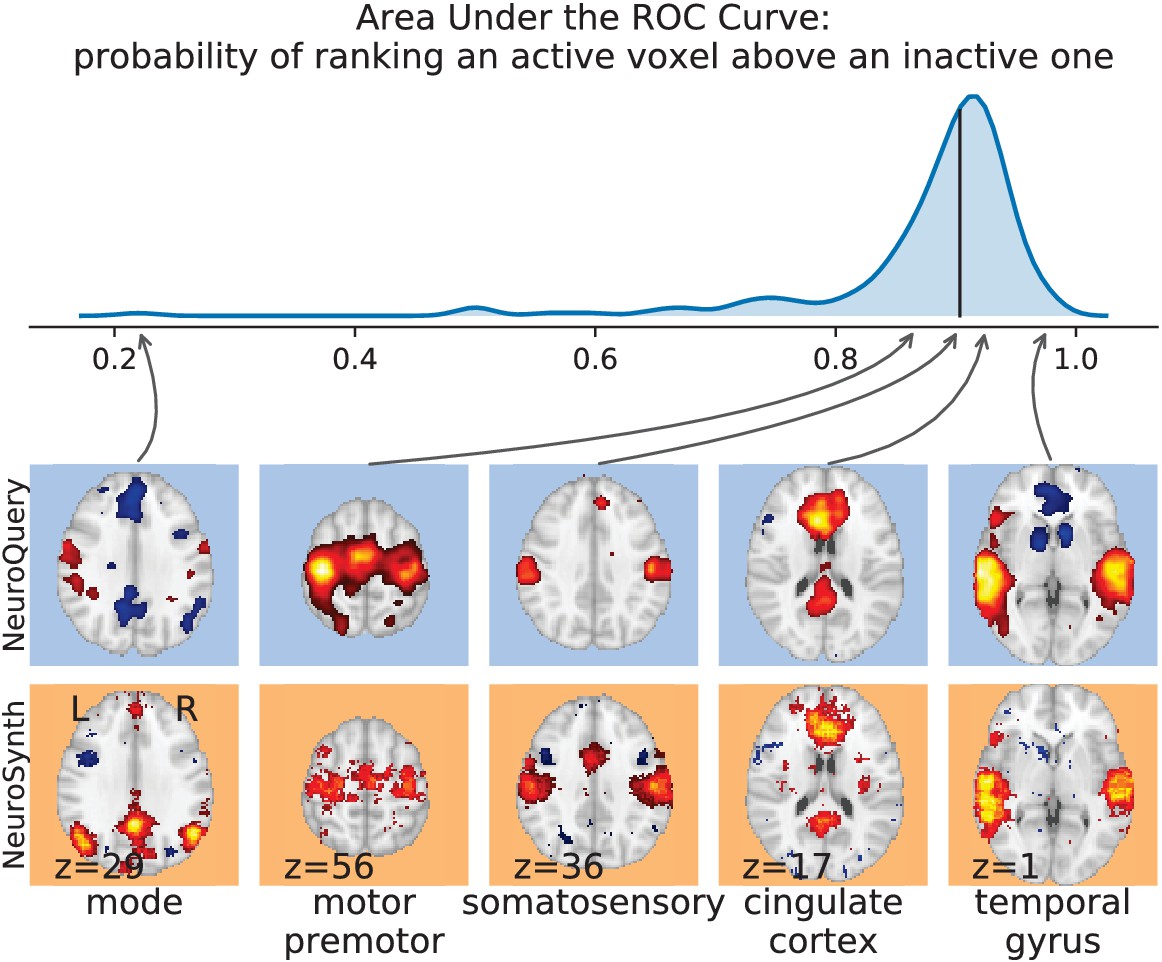
Comparison with NeuroSynth.
NeuroSynth maps are thresholded controlling the FDR at 1%. The 200 words with the largest number of active voxels are selected and NeuroQuery predictions are compared to the NeuroSynth activations by computing the Area Under the ROC Curve. The distribution of the AUC is shown on the top. The vertical black line shows the median (0.90). On the bottom, we show the NeuroQuery maps (first row) and NeuroSynth activations (second row) for the quartiles of the NeuroQuery AUC scores.
Figure 16
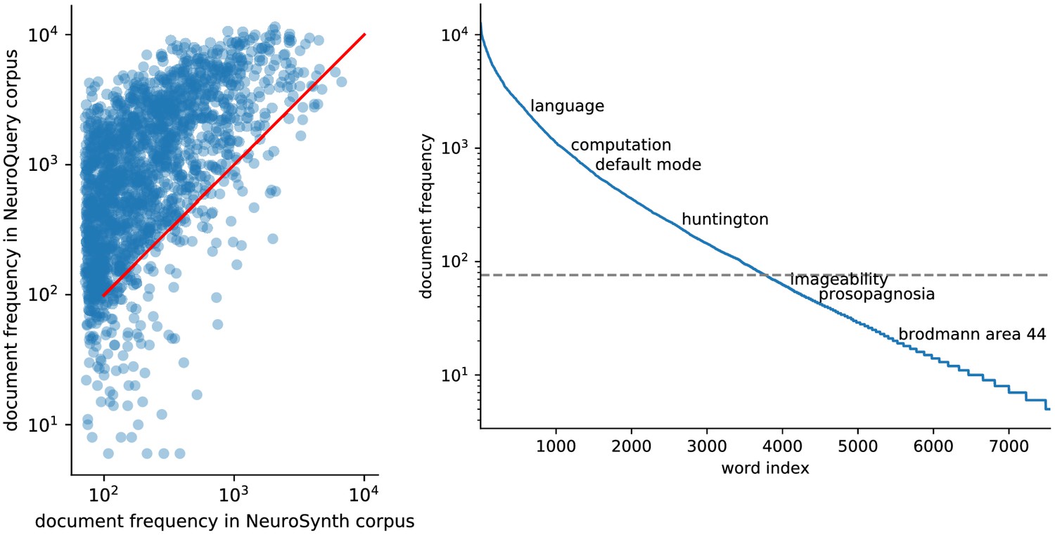
Right: benefit of using full-text articles.
Document frequencies (number of documents in which a word appears) for terms from the NeuroSynth vocabulary, in the NeuroSynth corpus ( axis) and the NeuroQuery corpus ( axis). Words appear in much fewer documents in the NeuroSynth corpus because it only contains abstracts. Even when considering only terms present in the NeuroSynth vocabulary, the NeuroQuery corpus contains over 3M term-study associations – 4.6 times more than NeuroSynth. Left: Most terms occur in few documents Plot of the document frequencies in the NeuroQuery corpus, for terms in the vocabulary, sorted in decreasing order. While some terms are very frequent, occurring in over 12 000 articles, most are very rare: half occur in less than 76 (out of 14 000) articles.
Figure 17
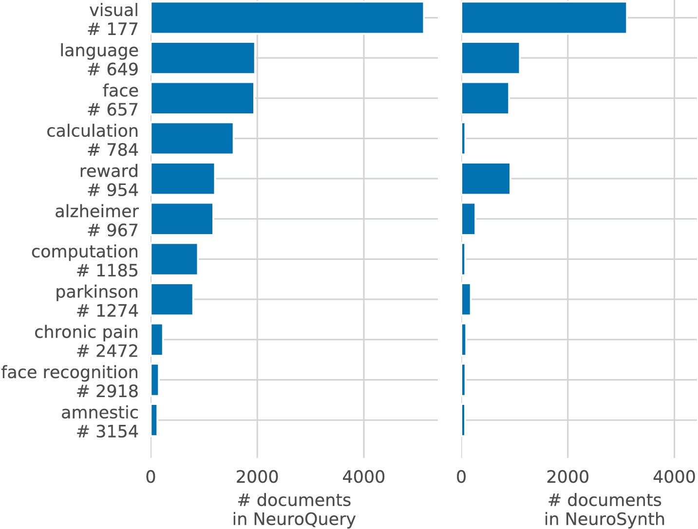
Document frequencies for some example words, in NeuroQuery’s and NeuroSynth’s corpora.
Figure 18
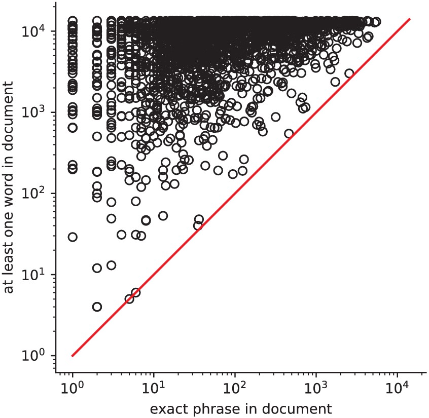
Occurrences of phrases versus its constituents How often a phrase from the vocabulary (e.g.
‘face recognition’) occurs, versus at least one of its constituent words (e.g. ‘face’). Expressions involving several words are typically very rare.
Figure 19

NeuroSynth posterior probability maps for ‘language’ (top) and ‘reward’ (bottom), using the full corpus.
Tables
Table 1
Diversity of vocabularies: there is no established lexicon of neuroscience, even in hand-curated reference vocabularies, as visible across CognitiveAtlas (Poldrack and Yarkoni, 2016), MeSH (Lipscomb, 2000), NeuroNames (Bowden and Martin, 1995), NIF (Gardner et al., 2008), and NeuroSynth (Yarkoni et al., 2011).
Our dataset, NeuroQuery, contains all the terms from the other vocabularies that occur in more than 5 out of 10 000 articles. ‘MeSH’ corresponds to the branches of PubMed’s MEdical Subject Headings related to neurology, psychology, or neuroanatomy (see Section 'The choice of vocabulary'). Many MeSH terms are hardly or never used in practice – For example variants of multi-term expressions with permuted word order such as ‘Dementia, Frontotemporal’, and are therefore not included in NeuroQuery’s vocabulary. Numbers above 25% are shown in bold.
| % of ↓ contained in → | Cognitive Atlas (895) | MeSH (21287) | NeuroNames (7146) | NIF (6912) | NeuroSynth (1310) | NeuroQuery(7547) |
|---|---|---|---|---|---|---|
| Cognitive Atlas | 100% | 14% | 0% | 3% | 14% | 68% |
| MeSH | 1% | 100% | 3% | 4% | 1% | 9% |
| NeuroNames | 0% | 9% | 100% | 29% | 1% | 10% |
| NIF | 0% | 12% | 30% | 100% | 1% | 10% |
| NeuroSynth | 9% | 14% | 5% | 5% | 100% | 98% |
| NeuroQuery | 8% | 25% | 9% | 9% | 17% | 100% |
Table 2
Number of extracted coordinate sets that contain at least one error of each type, out of 40 manually annotated articles.
The articles are chosen from those on which NeuroSynth and NeuroQuery disagree – the ones most likely to contain errors.
| False positives | False negatives | |
|---|---|---|
| NeuroSynth | 20 | 28 |
| NeuroQuery | 3 | 8 |
Table 3
Comparison with NeuroSynth.
‘voc intersection’ is the set of terms present in both NeuroSynth’s and NeuroQuery’s vocabularies. The ‘conflicting articles’ are papers present in both datasets, for which the coordinate extraction tools disagree, 40 of which were manually annotated.
| NeuroSynth | NeuroQuery | |
|---|---|---|
| Dataset size | ||
| articles | 14 371 | 13 459 |
| terms | 3 228 (1 335 online) | 7 547 |
| journals | 60 | 458 |
| raw text length (words) | ≈4 M | ≈75 M |
| unique term occurrences | 1 063 670 | 5 855 483 |
| unique term occurrences in voc intersection | 677 345 | 3 089 040 |
| coordinates | 448 255 | 418 772 |
| Coordinate extraction errors on conflicting articles | ||
| articles with false positives / 40 | 20 | 3 |
| articles with false negatives / 40 | 28 | 8 |
Table 4
Atlases included in NeuroQuery’s vocabulary.
Additional files
-
Source data 1
Source code for figures and tables.
- https://cdn.elifesciences.org/articles/53385/elife-53385-data1-v2.zip
-
Transparent reporting form
- https://cdn.elifesciences.org/articles/53385/elife-53385-transrepform-v2.docx
Download links
A two-part list of links to download the article, or parts of the article, in various formats.
Downloads (link to download the article as PDF)
Open citations (links to open the citations from this article in various online reference manager services)
Cite this article (links to download the citations from this article in formats compatible with various reference manager tools)
NeuroQuery, comprehensive meta-analysis of human brain mapping
eLife 9:e53385.
https://doi.org/10.7554/eLife.53385


