The frequency gradient of human resting-state brain oscillations follows cortical hierarchies
- Institute for Biomagnetism and Biosignalanalysis (IBB), University of Muenster, Germany
- Radboud University Nijmegen, Donders Institute for Brain, Cognition and Behaviour, Netherlands
- Psychology, University of Dundee, Scrymgeour Building, United Kingdom
- Centre for Cognitive Neuroimaging (CCNi), University of Glasgow, United Kingdom
- Otto-Creutzfeldt-Center for Cognitive and Behavioral Neuroscience, University of Muenster, Germany
Figures
Figure 1 with 2 supplements
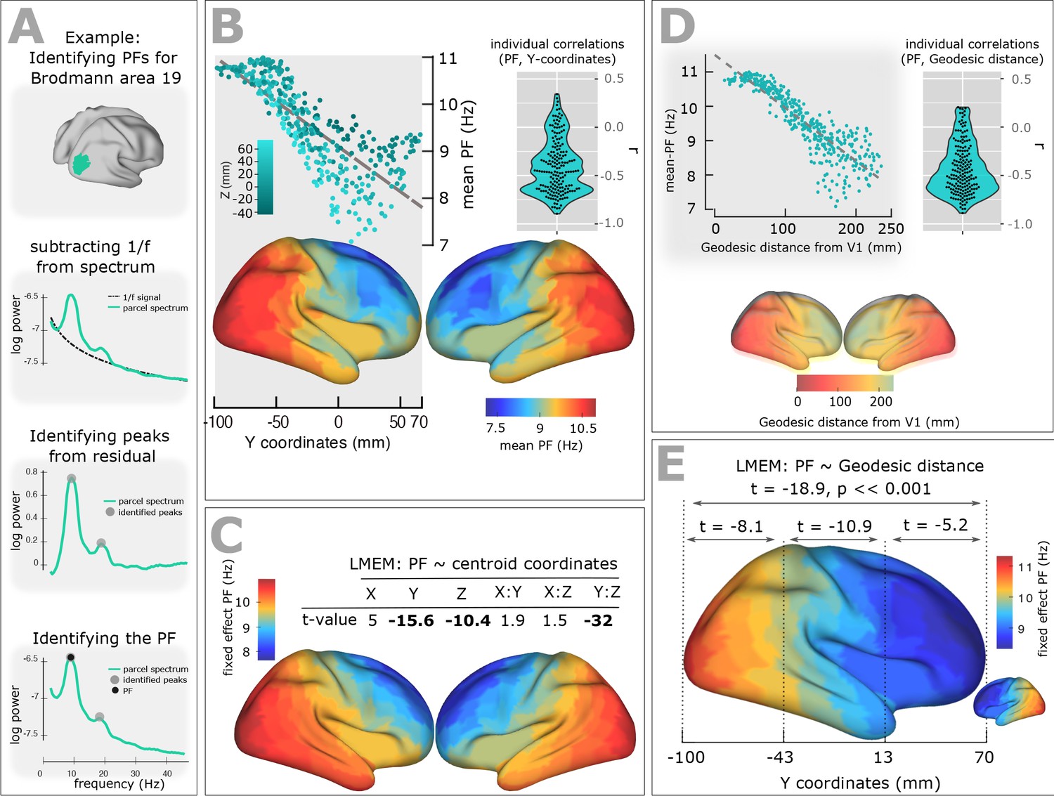
Spatial gradient of peak frequency (PF) across the human cortex follows the posterior-anterior hierarchy.
(A) Estimating the power spectrum for each cortical region, and identifying peak frequencies after fitting and subtracting the arrhythmic 1/f component. (B) Top-left panel shows the distribution of PF as a function of the ROI’s location along the y-axis of the coordinate system (posterior to anterior). Each point represents the trimmed mean across participants of the PF for one ROI (r = −0.84, p<<0.001). Points are colored according to their Z coordinates. Bottom panel: distribution of trimmed mean PFs across 384 cortical ROIs. Top-right panel: Individual level correlation values computed between PF and y-coordinates across ROIs (significant for 84% of participants, p<0.05) and their consistency across all individuals (t-value = −15.52, p<0.001). (C) Top panel: t-values obtained from linear mixed effect modeling of PF as a function of the coordinates of the ROI centroids. Bottom panel: cortical map of the corresponding fixed effect parameters (see Equation 2 for details). (D) Top-left panel: correlation between trimmed mean PF and geodesic distance (r = −0.89, p<<0.001). Top-right panel: individual correlation values (significant for 88% of participants, p<0.05) and their consistency across all individuals (t-value = −17.32, p<0.001). Bottom panel illustrates geodesic distance values mapped on the cortical surface. Geodesic distance was computed between centroid of all ROIs and the centroid of V1 and used this as a new axis to explain the posterior-anterior direction in the cortex. (E) LMEM of PF as a function of geodesic distance performed, separately, for all cortical ROIs, posterior-parietal ROIs (Y < −43 mm), central ROIs (−43 < Y < 13), and frontal ROIs (Y > 13). To assess the distribution of PF along the posterior-anterior axis while accounting for the inter-individual variability, LMEM was applied between the PF as a response variable and the geodesic distance values as an independent variable, and identified a highly significant gradient of PF along the specified geodesic distance (t = −18.9, p<<0.001). Furthermore, to test whether the spatial gradient of PF constantly exists in different areas of the cortex, the cortical surface was split to three equal, consecutive and non-overlapping windows (about 4 cm) based on its Y axis. For each window, LMEM was applied between PF and geodesic distance, and found a significant gradient (window 1: t = −8.1, window 2: t = −10.9, window 3: t = −5.2, all p<0.001). Indeed, our analysis demonstrates a significant organization of PF along the posterior-anterior direction for all windows indicating that this axis constitutes a systematic and constant gradient of PF.
Figure 1—figure supplement 1
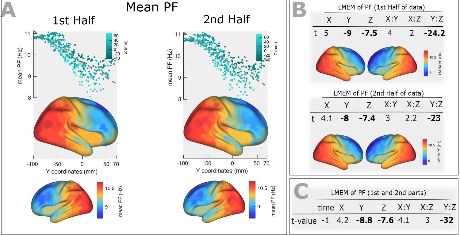
Stability of the PF gradient over time PF gradient along the posterior-anterior direction computed for 1 st and 2nd halves after splitting the time course to two equal segments.
(A) Top panels: correlation between trimmed mean PF (187 participants, 384 ROIs) and ROI’s location along the y-axis (posterior to anterior) computed for the first (r = −0.82, p<0.001) and second (r = −0.81, p<0.001) halves of the time course. Points are colored according to their Z coordinates. Bottom panel: trimmed mean PF values mapped on the cortex surface. (B) T-values obtained from linear mixed effect modeling of PF as a function of coordinates of the ROI centroids, obtained from the first half (top panel) and the second half (bottom panel) of the time course. Cortical maps below each table shows the fixed effects of the LMEM. (C) Linear mixed effect modeling of PF as a function of the time and centroid coordinates. We defined the time as a categorical variable (‘1 st half’, ‘2nd half’) and added it to our LMEM, where we defined PF as a function of centroid coordinates, their interactions and time. The statistical model showed a non-significant effect of time (t = −1, p>0.05) on our results. This analysis shows that the spatial gradient of PF along the posterior-anterior direction is stable over time.
Figure 1—figure supplement 2
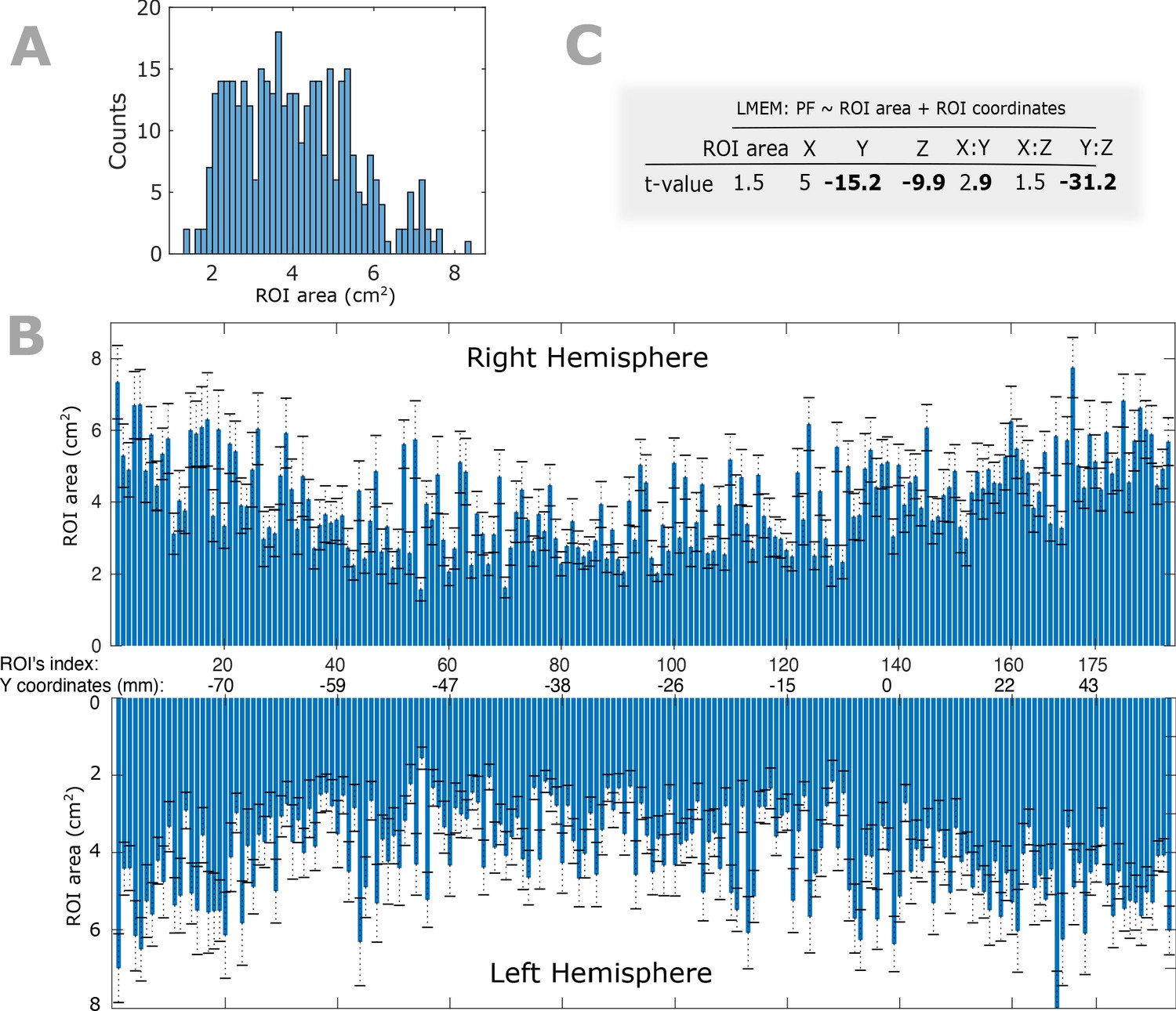
Within- and between-participant variability of ROIs’ size and their impact on PF gradient.
(A) Histogram of ROIs’ size for a given participant. (B) Bar plots depicting the between-participant variability of the ROIs’ area. Bars represent the mean and error bars show the standard deviation of a given ROI’s cortical area across all participants. In our main analysis, we down-sampled the individual cortical surfaces to 8196 vertices and 16384 (triangular) faces and co-registered to a finer version of Conte69 atlas. The atlas provides anatomical labels for each vertex but not for the faces. To obtain the area of a given ROI, we first assigned a label to each face based on the label of the nearest vertex (Euclidean distance was computed between centroid of the given face and all vertices) and summed across the area values of the identically labeled faces. (C) To assess the impact of ROI size on spatial gradient of PF, we used an LMEM according to Equation 1 of the manuscript where we included ROIs’ size as an additional fixed effect variable. We found no significant impact of ROIs’ size on spatial gradients of PF along the Z and Y axes (ROI size: t = 1.5, p>0.05; Y: t = −15.2, Z: t = −9.9, Y:Z: t = −31).
Figure 2

Spatial distribution of 1/f components (offset and slope) across human cortex.
(A) Top panel: t-values obtained from linear mixed effect modeling of 1/f offset as a function of the coordinates of ROI centroids. Bottom panel: cortical map of the corresponding fixed effects. (B) LMEM was applied on 1/f slope, analogous to the 1/f offset. The slope and offset of 1/f component were estimated for each ROI and participant, using the FOOOF package (see Materials and methods section for further details). (C) Correlation between trimmed mean PFres (187 participants, 384 ROIs) and ROI’s location along the y-axis (posterior to anterior) (r = −0.63, p<<0.001). The residual PF scores (PFres) were obtained after regressing out the contribution of 1/f offset and slope values (fixed effect) from PF, using LMEM. (D) t-values obtained from linear mixed effect modeling of PF as a function of the coordinates of the ROI centroids (LMEM; t-values: Y = −8.3, Z = −4.3, Y:Z = −16; all p<0.001). The cortical maps show the corresponding fixed effects.
Figure 3 with 2 supplements
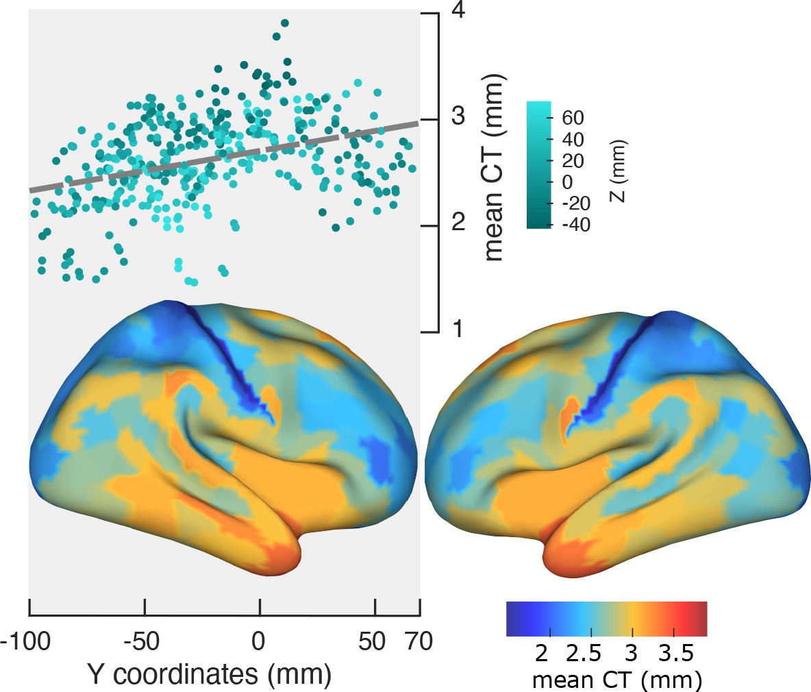
Spatial gradient of cortical thickness along the posterior-to-anterior direction.
Top panel: correlation between mean cortical thickness and ROI’s location along the y-axis (posterior to anterior) (r = −0.84, p<<0.001). Bottom panel: cortical map of trimmed mean PF across 384 cortical ROIs.
Figure 3—figure supplement 1

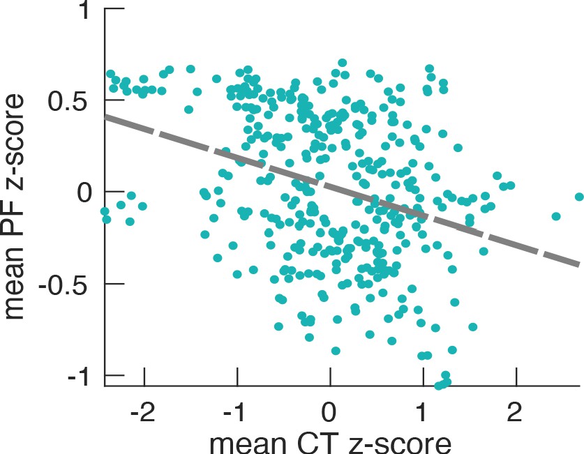
Relationship between PF (187 participants, 384 ROIs) and CT, after regressing out the effect of ROI coordinates.
We factored out the impact of ROI coordinates (x,y,z) from both PF and CT using LMEM according to Equation 1, and obtained the residuals, PFres and CTres. These residuals describe individual spatial variations of PF and CT that cannot be explained by a linear model of their spatial location. We again applied LMEM defining PFres as a function of CTres and found a significant relationship (LMEM: t = −6.9, p<<0.001). The scatter plot represents the relationship between the mean PFres and the mean CTres across cortical ROIs. This significant relationship demonstrates that they are more directly related to each other than can be explained by their individual dependency on location (x,y,z). This result proposes that peak frequency is related to structural features that likely represent cortical hierarchies.
Figure 3—figure supplement 2
Relationship between PF (187 participants, 384 ROIs) and CT.
The scatter plot represents the dependency between the trimmed mean PF and the trimmed mean-CT and their correlation (r = −0.14, p<0.001). This low correlation (although very significant) actually reflects the fact that correlation analysis is not optimal in this case. It does not take into consideration the variability between participants (e.g. the fact that some participants have an overall higher occipital alpha frequency compared to others). This is also one of the reasons for the large scattering of values in the plot. Therefore, LMEM is the preferred statistical tool because it models specifically the inter-individual differences and, as a result, leads to more robust and highly significant results.
Figure 4 with 2 supplements
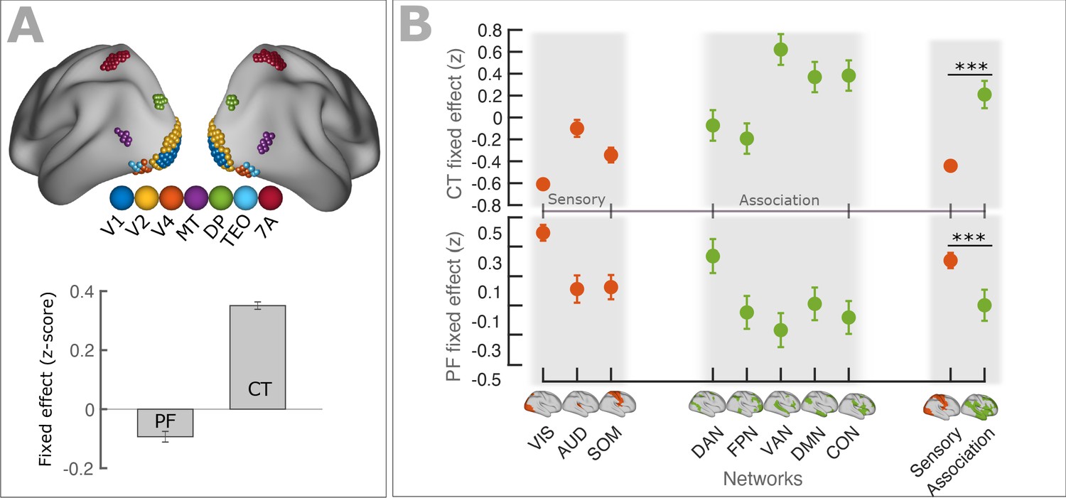
PF and CT variation along the cortex follows anatomical hierarchies.
(A) Top panel: Schematic representation of seven regions (V1, V2, V4, MT, DP, TEO, 7A) used for defining visual hierarchy. Bottom panel: Each bar shows the fixed effect of the LMEM where the PF/CT was defined as a response variable and the visual hierarchy as an independent variable. We found a significant decrease of PF (t = −10.1, p<<0.001) but a significant increase of CT (t = 54.9, p<<0.001) along the visual hierarchy. To impose the hierarchical order of the seven ROIs in an LMEM, we defined a seven-element hierarchy vector for each participant and hemisphere (V = [1, 2, 3, …, 7]), whose elements refer to the hierarchical level of the corresponding ROI. The random effect was specified as in Equation 1. PF/CT values were standardized before LMEM analysis. This model tests the significance of PF/CT changes along the specified hierarchy. (B) Fixed effect per network obtained from linear mixed effect modeling of CT (top panel) and PF (bottom panel) as a function of networks (independent variable), where networks were specified as a categorical variable. The random structure was defined as in Equation 1. Fixed effect per network indicates the effect of that network on PF/CT. The network variable was defined as a categorical variable by assigning cortical regions to eight functional resting-state networks comprising three sensory (‘VIS’, visual; ‘AUD’, auditory; and ‘SOM’, somatomotor) and five association (‘DAN’, dorsal 670 attention; ‘FPN’, frontoparietal; ‘VAN’, ventral attention; ‘DMN’, default mode; and ‘CON’, cingulo-opercular) networks. We applied ANOVA on LMEM fit and computed F-stat for the fixed effect. (PF: F-stats = 264, p<<0.001; CT: F-stats = 746, p<<0.001). PF values were significantly lower in association RSNs (except for DAN) than in sensory RSNs (t = −11.1, p<<0.001), whereas CT values were significantly higher in association RSNs than in sensory RSNs (t = 14.1, p<<0.001). Error bar indicates the lower and upper bounds of LMEM for the fixed effect.
Figure 4—figure supplement 1
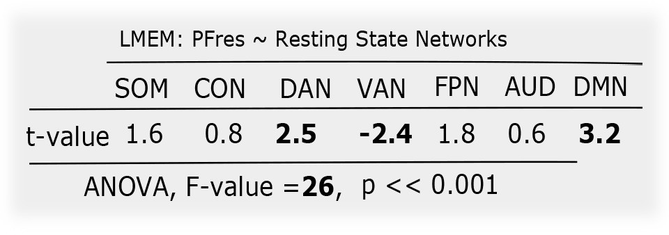
Distribution of the location independent PF (PFres) among resting state networks.
T-values obtained from linear mixed effect modeling of the location independent PF among resting state networks. The network variable was defined as described in Figure 4. Here, we asked the question of whether the PF differs between resting state networks irrespective of its location? To answer this, we first regressed out from PF the changes that can be explained by linear dependencies on x,y,z, using LMEM, and again performed LMEM analysis (between PF and networks) as described for Figure 4. Interestingly, we found a significant difference among networks for PF. This was the case when looking at the standard resting-state networks and also when testing sensory against association areas. These results indicate that, beyond a global effect of location, networks still differ significantly in PF after removing the linear effects of location.
Figure 4—figure supplement 2
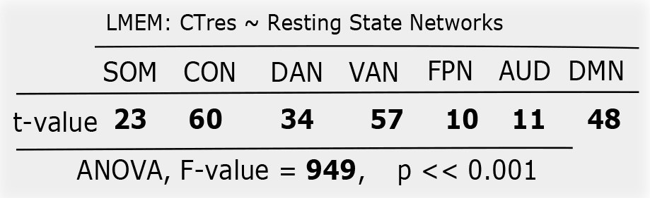
Distribution of location independent CT (CTres) among resting state networks.
Similar to Figure 4—figure supplement 1, LMEM was performend on CT values, and found a significant difference between network. This result turns out that the significant impact of networks on CT is independent of location.
Figure 5
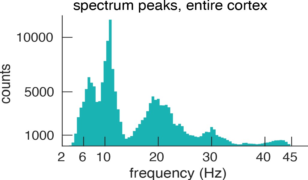
Histogram of spectral peaks.
Histogram of all detected spectral peaks (across ROIs and participants) delineates the classical frequency bands used in the EEG and MEG literature (theta 3.5–7.5 Hz, alpha 8.5–13 Hz, low-beta 15–25 Hz and high-beta 27.5–34).
Figure 6 with 2 supplements
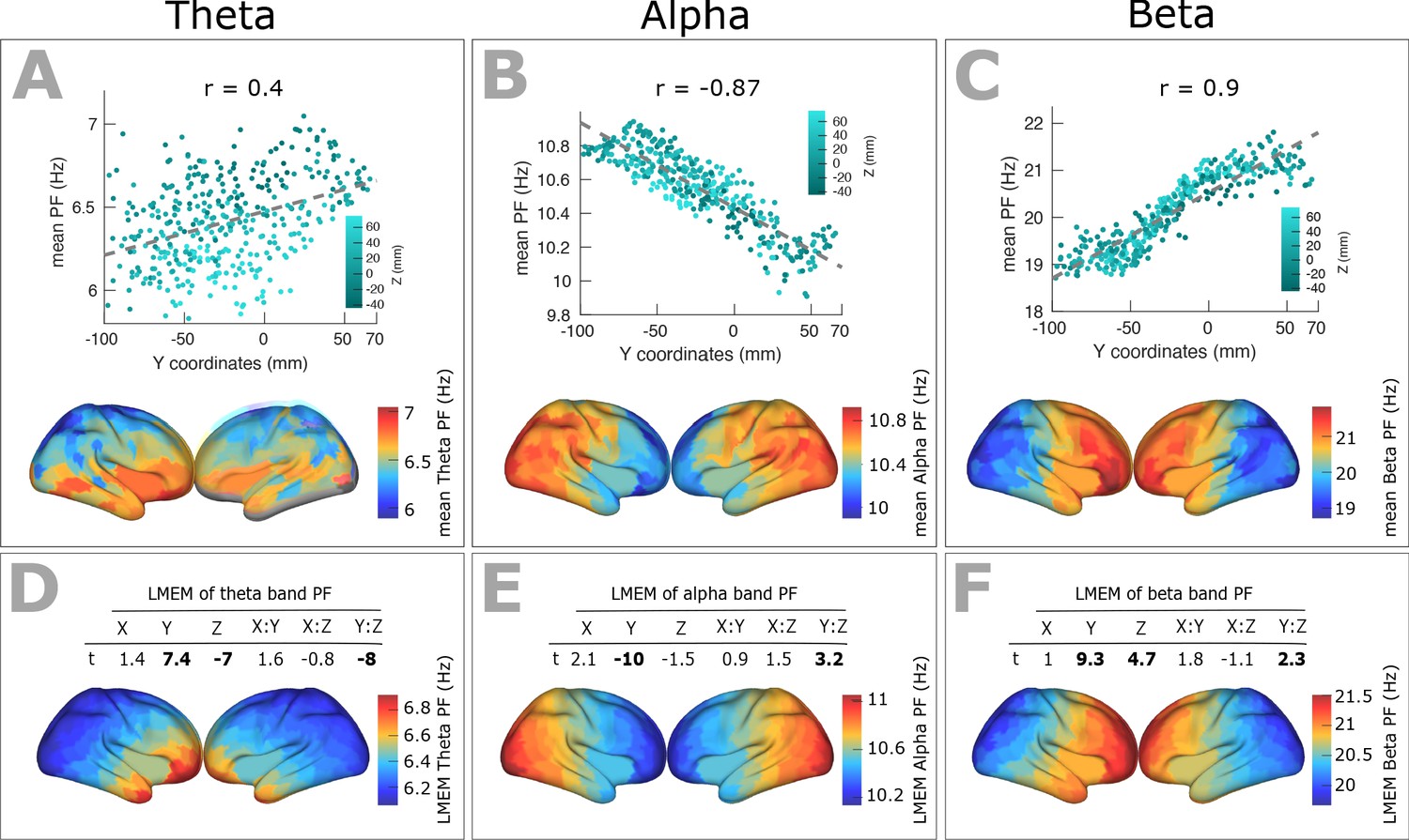
Spatial gradients of band-specific PFs across human cortex follows the posterior-anterior direction.
(A, B, and C) Top panel: Dependency between the trimmed mean of band-specific PF (187 participants, 384 ROIs) and the ROI’s location along the y-axis (posterior to anterior) for theta (r = 0.4, p<0.001), alpha (r = −0.87, p<0.001), and beta (r = 0.9, p<0.001) bands, respectively. Points are colored according to their Z coordinates. Bottom panel: distribution of trimmed mean band-specific PFs across 384 cortical ROIs. (D, E, and F) Top panel: t-values obtained from linear mixed effect modeling of band-specific PF (theta, alpha, and beta bands, respectively) as a function of the coordinates of the ROI centroids. Bottom panel: cortical map of the corresponding fixed effect parameters (see Equation 2 for details).
Figure 6—figure supplement 1
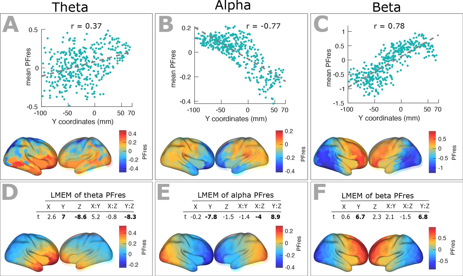
Spatial gradients of band-specific PF across the cortex after factoring out the impact of 1/f components (offset and slope).
(A) Top panel: Scatter plots representing the relationship between trimmed mean PFres (187 participants, 384 ROIs) and ROI’s location along the y-axis for theta band (r = 0.3, p<0.001), together with corresponding cortical map of trimmed mean PFres.
Panels (B) and (C) show the same results for alpha (r = −0.77, p<<0.001), and beta (r = 0.78, p<<0.001) frequency ranges. The residual PF scores (PFres) were obtained after regressing out the contribution of 1/f offset and slope values (fixed effect) from band-specific PF, using LMEM. (D) Top panel: t-values obtained from linear mixed effect modeling of band-specific PFres as a function of the coordinates of the ROI centroids for theta band (LMEM; t-values: Y = 7, Z = −8.6, Y:Z = −8.3; all p<0.001). Bottom panel: cortical map of the corresponding fixed effect parameters (see Equation 2 for details). Similarly, panels (E) and (F) show the results for alpha (LMEM; t-values: Y = −7.8, X:Z = −4, Y:Z = 8.9; all p<0.001), and beta (LMEM; t-values: Y = 6.7, Y:Z = 6.8; all p<0.001) frequency ranges, respectively. These analyses demonstrate that the spatial gradient of band-specific PFs is independent of spatial changes of 1/f slope and offset.
Figure 6—figure supplement 2

Dependency between band-specific PF and CT.
Scatter plots show the relationship between trimmed mean band-specific PF and mean CT for theta (A), alpha (B), and beta (C) frequency ranges. Robust correlation was computed between trimmed mean band-specific PF and mean CT. LMEM was applied across all cortical regions defining individual band-specific PF as a function of individual CT (fixed effects) while accounting for between-individual variability (random effect). Both correlation and LMEM analyses identified a significant positive relationship for theta and beta bands but a significant negative relationship for alpha band. This analysis shows that the dependency between PF and CT is frequency specific.
Additional files
Download links
A two-part list of links to download the article, or parts of the article, in various formats.
Downloads (link to download the article as PDF)
Open citations (links to open the citations from this article in various online reference manager services)
Cite this article (links to download the citations from this article in formats compatible with various reference manager tools)
The frequency gradient of human resting-state brain oscillations follows cortical hierarchies
eLife 9:e53715.
https://doi.org/10.7554/eLife.53715


