The head direction circuit of two insect species
- School of Informatics, University of Edinburgh, United Kingdom
- Lund Vision Group and NanoLund, Lund University, Sweden
Figures
Figure 1 with 1 supplement
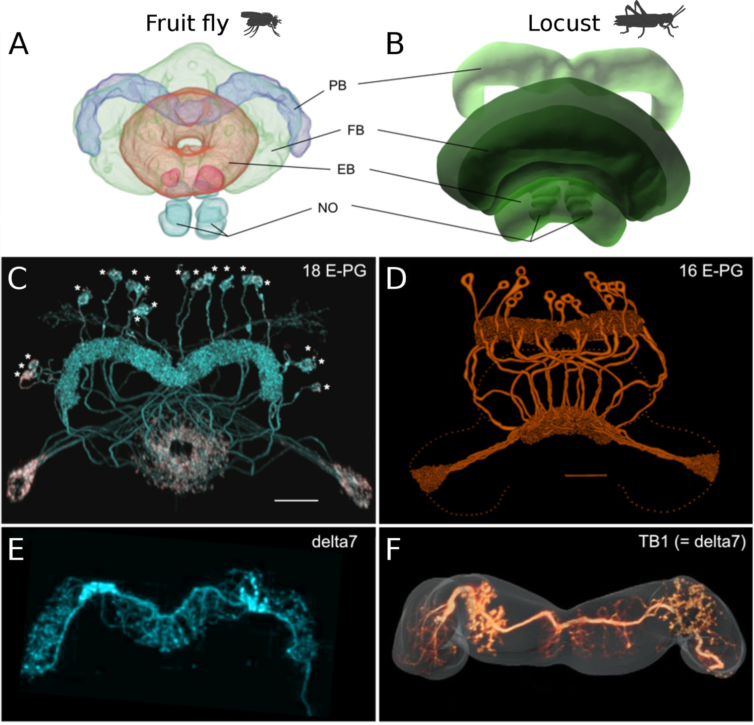
Anatomical differences between two species.
There are three apparent differences between the CX of the fruit fly (Drosophila melanogaster) and the desert locust (Schistocerca gregaria). (A, B) The ellipsoid body in the fruit fly has a toroidal shape while in the locust is crescent-shaped so its two ends are separate. (C, D) The protocerebral bridge consists of 18 glomeruli and 18 corresponding E-PG and P-EG neurons in the fruit fly (see Table 3) while in the locust there are 16 glomeruli and neurons innervating them. (E, F) The Delta7 neurons in the fruit fly have postsynaptic domains along the whole length of their neurite while in the desert locust only in specific sections with gaps in between.
© 2018 Wiley Periodicals, Inc. Panel A, C and E are reproduced and adapted from Wolff and Rubin, 2018 with permission from Wiley Periodicals, Inc. They are not covered by the CC-BY 4.0 licence and further reproduction of this panel would need permission from the copyright holder.
© 2009 Insect Brain Database. Panel B is an original image only available for non-commercial use from El Jundi et al., 2009 with permission from Insect Brain Database, https://insectbraindb.org. They are not covered by the CC-BY 4.0 licence and further reproduction of this panel would need permission from the copyright holder.
© 1998 Wiley-Liss, Inc. Panel D is reproduced from Vitzthum and Homberg, 1998 with permission from Wiley-Liss, Inc. They are not covered by the CC-BY 4.0 licence and further reproduction of this panel would need permission from the copyright holder.
© 2015 Wiley Periodicals, Inc. Panel F is reproduced from Figure 1J of Beetz et al., 2015 with permission from Wiley Periodicals, Inc. They are not covered by the CC-BY 4.0 licence and further reproduction of this panel would need permission from the copyright holder.
Figure 1—figure supplement 1
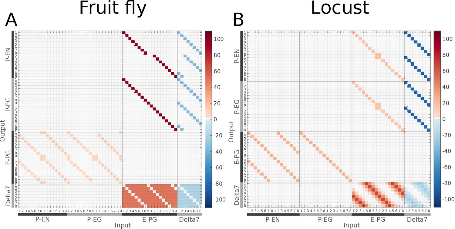
Connectivity matrices of the two species.
Connectivity matrices of the two species. The connectivity matrices derived by the exact neuronal projections of (A) the fruit fly (Drosophila melanogaster) and (B) the desert locust (Schistocerca gregaria), respectively. The difference in the distribution of Delta7 neuron synaptic domains is evident at the lower right part of the images. Synaptic strength is denoted by colour in units of postsynaptic current equivalents as described in section Materials and methods.
Figure 2
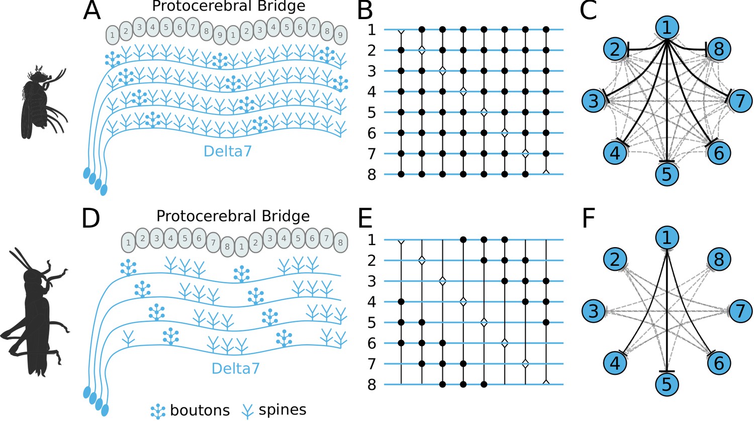
Effective connectivity of the inhibitory (Delta7) neurons.
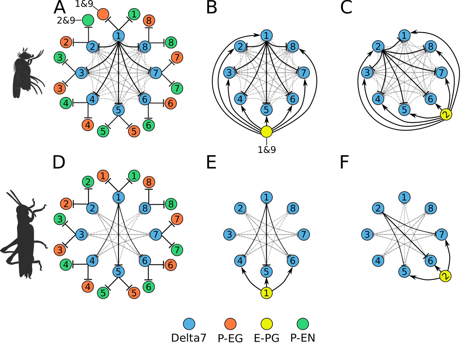
On the top row is the fruit fly circuit, on the bottom row is the locust circuit. In A and D, four examples of how the eight types of Delta7 neurons innervate the PB are illustrated. In both species, presynaptic domains are separated by seven glomeruli. (B and E) Effective connectivity. Each horizontal blue line represents one Delta7 neuron. Vertical lines represent axons, with triangles indicating outputs from Delta7 neurons and filled circles representing inhibitory synapses between axons and other Delta7 neurons. (C and F) Alternative depiction of the circuit in graph form with blue circles representing Delta7 neurons and lines representing inhibitory synapses between pairs of neurons. Each Delta7 neuron inhibits all other Delta7s in the fruit fly (C), but only more distant Delta7s in the locust (F).
Figure 3 with 3 supplements
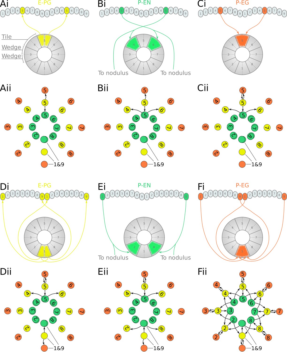
Projection patterns of the excitatory portion of the fruit fly circuit.
(Ai–Fi) Examples of E-PG (combined E-PG and E-PGT, see Table 3), P-EN and P-EG neurons with their synaptic domains and projection patterns. (Aii–Cii) Step by step derivation of the effective circuit as a directed graph network (see main text for a complete description). Each coloured disc represents a group of neurons with arrows representing excitatory synaptic connections. Pairs of E-PG and P-EG neurons can be considered to act as single units connecting the respective tile to equally numbered PB glomeruli in both hemispheres, while P-EN neurons are shown overlapped because each receives input only from its contralateral nodulus. (Dii–Eii) The connectivity also allows neurons innervating glomeruli 1 and 9 to act as a single unit. (Fii) Depiction of the complete effective connectivity of the excitatory circuit, which has an eight-fold radial symmetry.
Figure 3—figure supplement 1
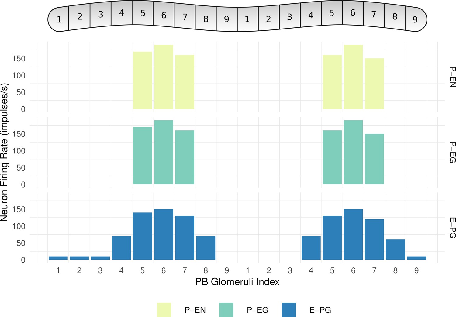
Neuronal activity across PB glomeruli.
The neuronal activity of P-EN, P-EG and E-PG neurons innervating the glomeruli of the PB for the simulated model of the fruit fly. The activity ‘bump’ is centred around identically numbered glomeruli on the two hemispheres.
Figure 3—figure supplement 2
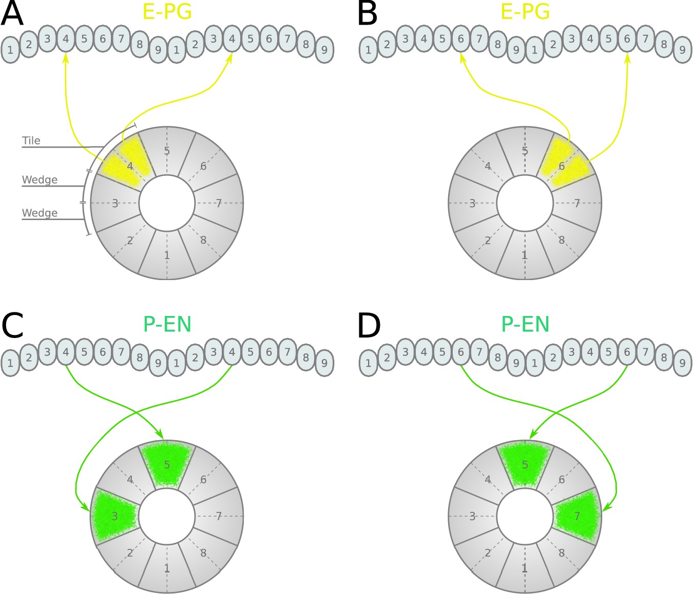
Neuronal projections in the fruit fly.
(A, B) Examples of the projection patterns of E-PG neurons (combined E-PG and E-PGT, see Table 3). (C, D) Examples of P-EN neurons with their synaptic domains and projection patterns (see main text for detailed description).
Figure 3—video 1
Animation illustrating the operation of the excitatory portion of the fruit fly circuit.
Figure 4 with 3 supplements

Projection patterns of the excitatory portion of the locust circuit.
(Ai–Ei) Examples of E-PG, P-EN and P-EG neurons with their synaptic domains and projection patterns. (Aii–Eii) Step by step derivation of the effective circuit (see main text for a complete description). Each coloured disc represents a group of neurons with arrows representing excitatory synaptic connections. Pairs of E-PG and P-EG neurons can be considered to act as single units connecting the respective tile to equally numbered PB glomeruli in both hemispheres, while P-EN neurons are shown overlapped because each receives input only from its contralateral nodulus. Note that the numbering of the EB slices is conceptual and arbitrary, chosen to assist description of the circuit organisation; what matters for the connectivity is the overlap of the synaptic domains in the EB and not the particular numbering choice. (Fi) The complete effective connectivity of the locust excitatory circuit closely resembles that of the fruit fly. (Fii) Between octants 1 and 8, the locust circuit obtains functional connectivity from P-EN8 to ‘neighbouring’ E-PG1 (red dashed arrow) via three actual connections: P-EN8 to E-PG8 to P-EN1 to E-PG1 (black arrows); and equivalently for P-EN1 to E-PG8.
Figure 4—figure supplement 1
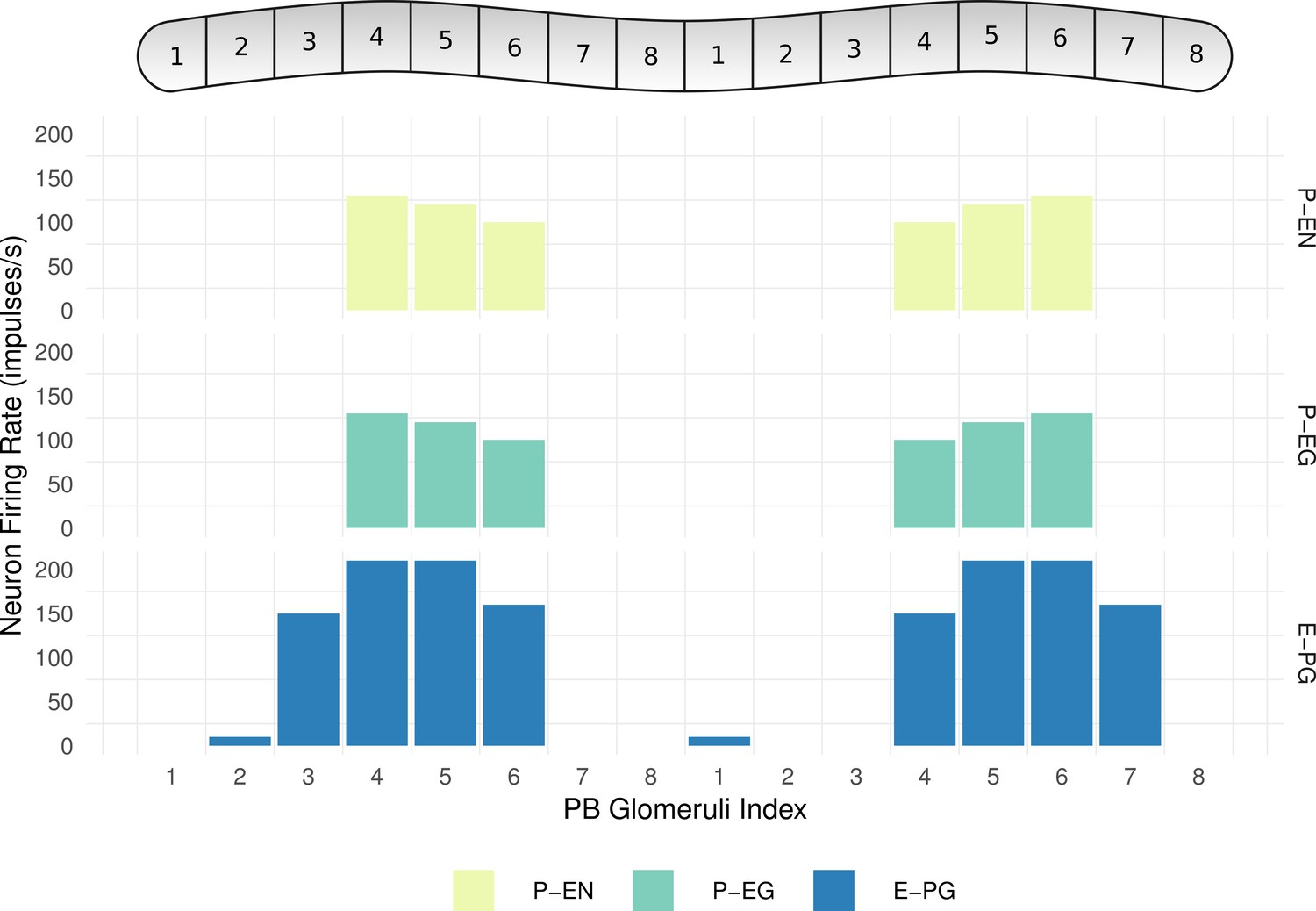
Neuronal activity across PB glomeruli.
The neuronal activity of P-EN, P-EG and E-PG neurons innervating the glomeruli of the PB for the simulated model of the locust. The activity ‘bump’ is centred around identically numbered glomeruli on the two hemispheres.
Figure 4—figure supplement 2
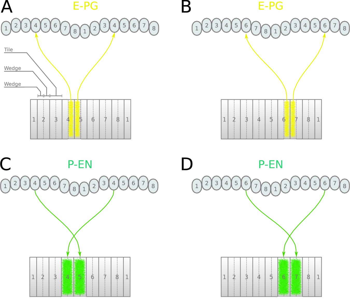
Neuronal projections in the locust.
Examples of the projection patterns of E-PG (A, B) and P-EN (C, D) neurons in the locust. The anatomy and projection patterns differ from those in the fruit fly (see main text for detailed description).
Figure 4—video 1
Animation illustrating the operation of the excitatory portion of the locust circuit.
Figure 5
Combined excitatory and inhibitory portion of the ring attractors.
Explanatory drawings of the connectivity of the inhibitory portion with the excitatory portion of the circuit for the fruit fly (A–C) and the locust (D–F). Each coloured disc represents one or more neurons with lines representing synaptic connections. (A) Conceptual depiction of effective global inhibition in the fruit fly. The connectivity of E-PG neurons is shown for two neurons only (B,C and E,F). In this conceptual effective connectivity drawing, E-PG neurons appear to be located on the one side of the ring making synapses around the ring. However, anatomically each E-PG neuron innervates one glomerulus where it makes all its synapses with postsynaptic Delta7 neurons that run along the PB.
Figure 6
Relative synaptic strengths.
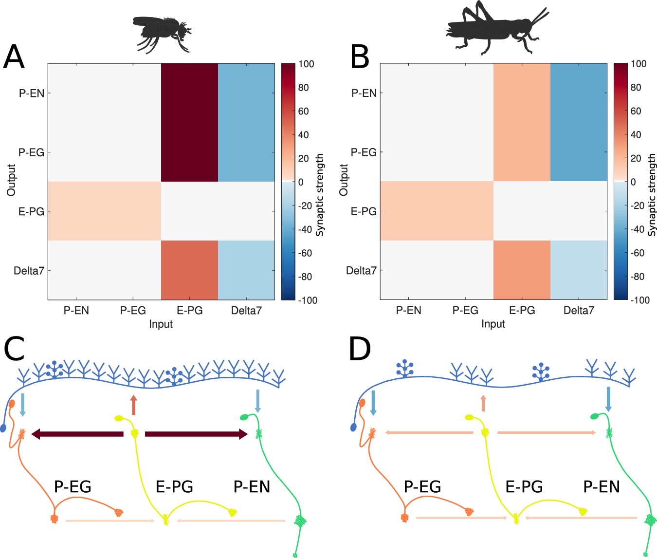
Graphical depiction of the synaptic strengths between classes of neurons. (A,C) For the fruit fly ring attractor circuit. (B,D) For the desert locust ring attractor circuit. Synaptic strengths are denoted by colour in panels A and B. In panels C and D, synaptic strengths between neurons are indicated by arrow colour and thickness in scale. Note that in the locust the synaptic strengths shown for Delta7 neurons are the peak values of the Gaussian distributed strengths shown in Figure 1—figure supplement 1.
Figure 7 with 1 supplement
Response to abrupt stimulus changes and tuning curves of neurons.
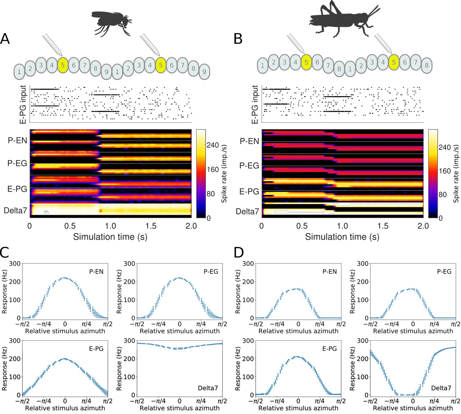
(A and B) The raster plots of the stimuli used to drive the ring attractor during the simulation are shown on top and the spiking rate activity of each neuron at the bottom. In the beginning of the simulation the stimulus spiking activity sets the ring attractor to an initial attractor state. A ‘darkness’ period of no stimulus follows. Then a second stimulus corresponding to a sudden change of heading by 120° is provided. In the lower parts of A and B, the spiking activity of each neuron, filtered along the time axis by a Gaussian low-pass filter with window of and , is shown colour coded. The order of recorded neurons is the same as shown in the connectivity matrices (Figure 1—figure supplement 1). (A) Response of the fruit fly ring attractor to sudden change of heading. (B) Response of the locust ring attractor to sudden change of heading. Even though the activity ‘bump’ in the locust model tends to start transitioning sooner, the fruit fly model completes the transition faster. (C and D) Response of individual neuron types to different stimuli azimuths (n = 40 trials in each condition). The mean and standard deviation are indicated by the error bars at the sampled azimuth points. Peak activity has been shifted to 0°. (C) Tuning curves for the fruit fly and (D) tuning curves for the locust.
Figure 7—figure supplement 1
Response of spiking and rate-based models to step change of heading.
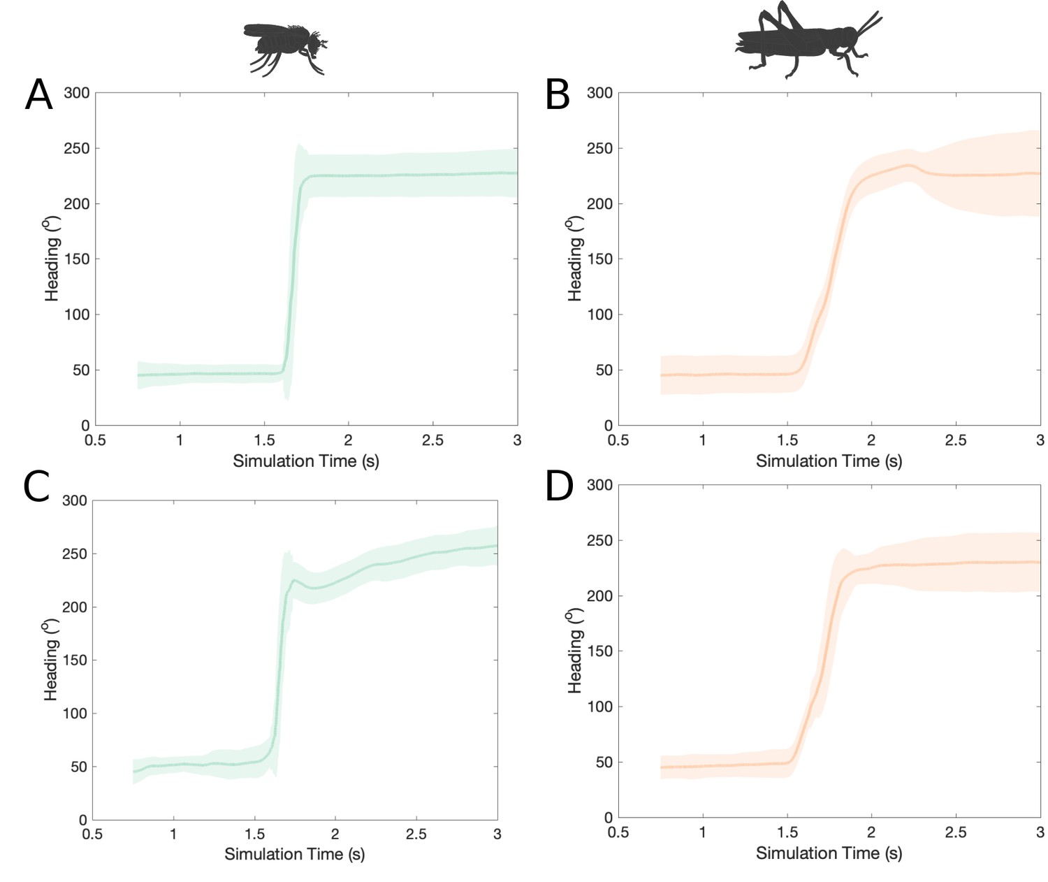
The mean activity ‘bump’ heading and corresponding standard deviation for the fruit fly and the locust models across time when stimulated with a step change of heading by 180° (80 trials each). (A, B) using spiking neuron models; (C, D) using rate-based neuron models. The activity ‘bump’ moves gradually to the new heading azimuth in the locust models (B, D) while it moves instantaneously in the fruit fly models (A, C). Note that in A and C, the transition slope does not appear exactly vertical (instantaneous) because it is the mean of multiple trials with the transition for each trial occurring with a small time lag in respect to the others.
Figure 8
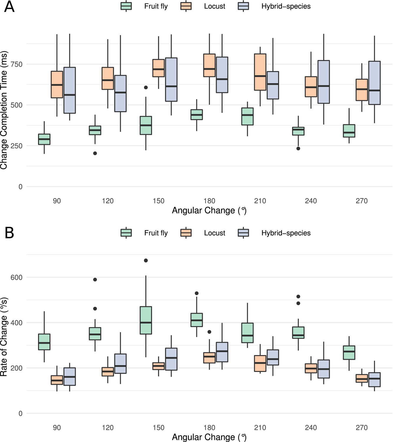
Transition time and rate of the heading signal.
(A) Time required from the onset of the stimulus until the heading signal settles to its new state. The abscissa (horizontal axis) displays the azimuthal difference between initial and target azimuth. (B) The maximum rate of angular change each model can attain computed as the ratio of shortest angular change of stimulus divided by transition duration. The values for different magnitudes of heading change are depicted as medians. The boxes indicate the 25th and 75th percentiles while the whiskers indicate the minimum and maximum value in the data after removal of the outliers (black dots). ‘Hybrid-species’ is the combination of the fruit fly model with the locust inhibition pattern.
Figure 9
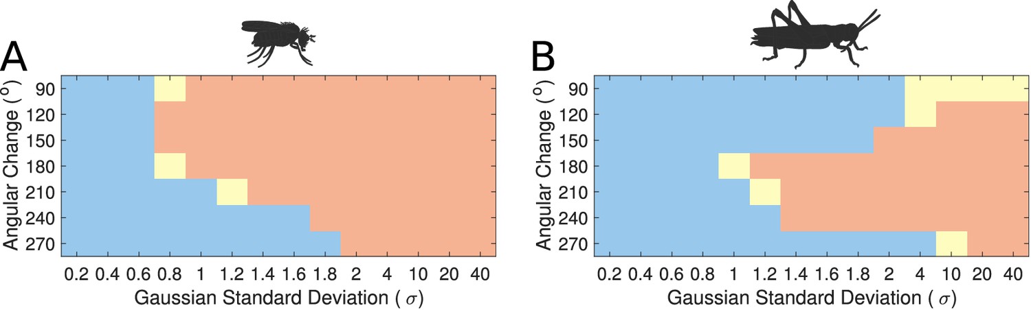
Transition regime as function of inhibitory uniformity.
Heading signal transition regime for (A) the fruit fly ring attractor circuit and (B) the desert locust ring attractor circuit. Blue denotes gradual transition of the heading signal, orange denotes abrupt transition (jump), and yellow marks trials that were producing both gradual and abrupt transitions (for definitions see section Materials and methods).
Figure 10
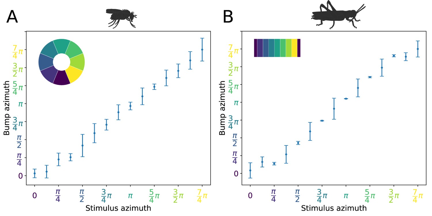
Distribution of activity ‘bump’ locations.
The distribution of azimuthal location of the heading signal 3 s after stimulus removal is plotted. On the abscissa (horizontal axis), the azimuth where the stimulus is applied is shown. On the ordinate (vertical axis), the mean location and standard deviation of the activity ‘bump’ azimuth, 3 s after the stimulus is removed, are shown. (A) for the fruit fly and (B) for the locust. Inset images depict the corresponding EB tiles in colour. Smaller standard deviation corresponds to the ‘bump’ settling more frequently to the same azimuth. This is the case when the stimulus is applied near an attractor state. Applying the stimulus equidistantly from two attractor states results in a movement of the ‘bump’ to either of them and hence the increased standard deviation. In the locust when stimulating the ring attractor at one of the attractor states the ‘bump’ tends to settle at it, indicated by the reduced standard deviation at these locations. In the fruit fly, the activity ‘bump’ is prone to noise and not as stable, thus the standard deviation is not as modulated. This means that the locust attractor states are more stable resulting to the smaller dispersion of ‘bump’ location.
Figure 11
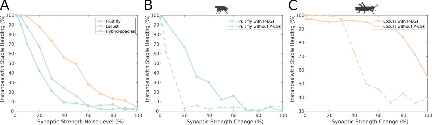
Effect of synaptic efficacy heterogeneity on ring attractor stability.
(A) Stability of the ring attractor heading signal for the fruit fly, locust and hybrid-species (fruit fly with localised inhibition) model as a function of heterogeneity in the synaptic efficacies across all synapse types (modelled as additive white Gaussian noise). (B, C) Stability of the ring attractor heading signal as a function of structural asymmetry introduced by deviating synaptic efficacies between P-EN and E-PG neurons when the circuit includes the P-EG neurons versus when they are removed. In all three plots, the percentage of trials that result in a stable activity ‘bump’ is shown. On the horizontal axis the absolute value of percentile synaptic strength change is shown. Number of trials n = 100 for each level of noise. With P-EG neurons both ring attractors are more tolerant to such structural asymmetries. The locust ring attractor is more robust to both types of structural noise.
Figure 12 with 1 supplement
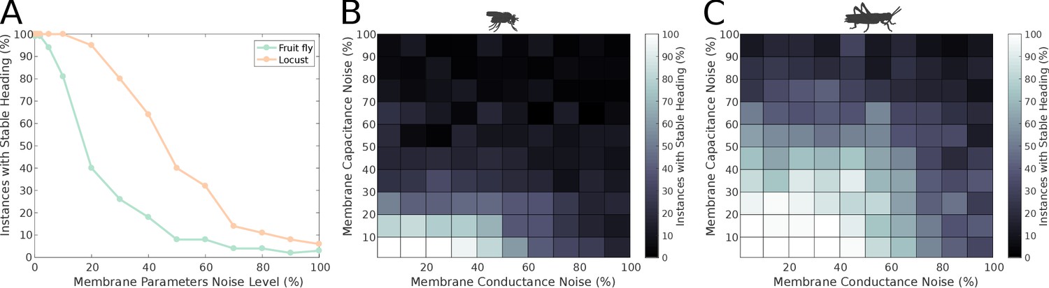
Effect of membrane parameter heterogeneity on ring attractor stability.
(A) Stability of the ring attractor heading signal for the fruit fly and the locust model when the membrane properties are heterogeneous across the neuronal population. (B, C) Stability of the ring attractor heading signal when the level of noise on conductance and capacitance is varied independently. In all three plots, the percentage of trials that result in a stable activity ‘bump’ as a function of heterogeneity in cell membrane properties is shown (number of trials n = 50 for each condition). The locust ring attractor is more robust to white Gaussian noise in both conductance and capacitance. In both cases, the activity ‘bump’ is more tolerant to conductance variation than capacitance.
Figure 12—figure supplement 1
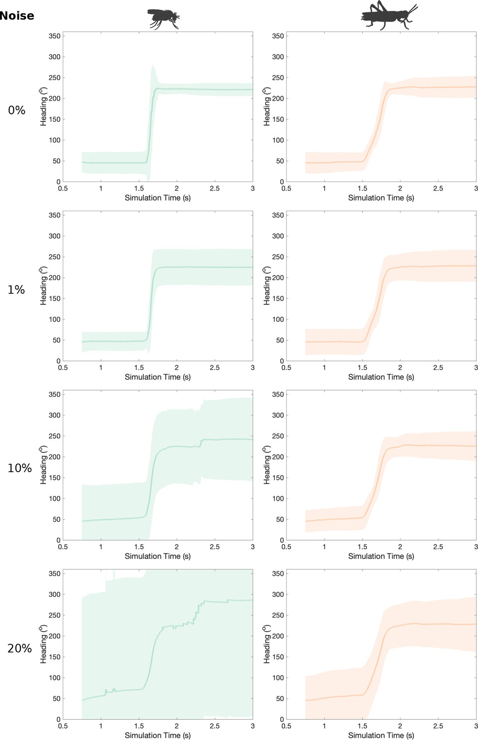
Effect of cell membrane parameter heterogeneity to transition regime.
The difference in the heading signal transition is present at different amounts of heterogeneity in neuron membrane parameters. As neuronal parameters deviate from their nominal values, from top to bottom, the stability of the heading signal deteriorates. The noise added to each membrane property (conductance and capacitance) was chosen from a normally distributed pseudorandom generator with sigma values in the range from 0 to the nominal value of the parameter and the resulting values were clipped to 0 so they are never negative.
Figure 13
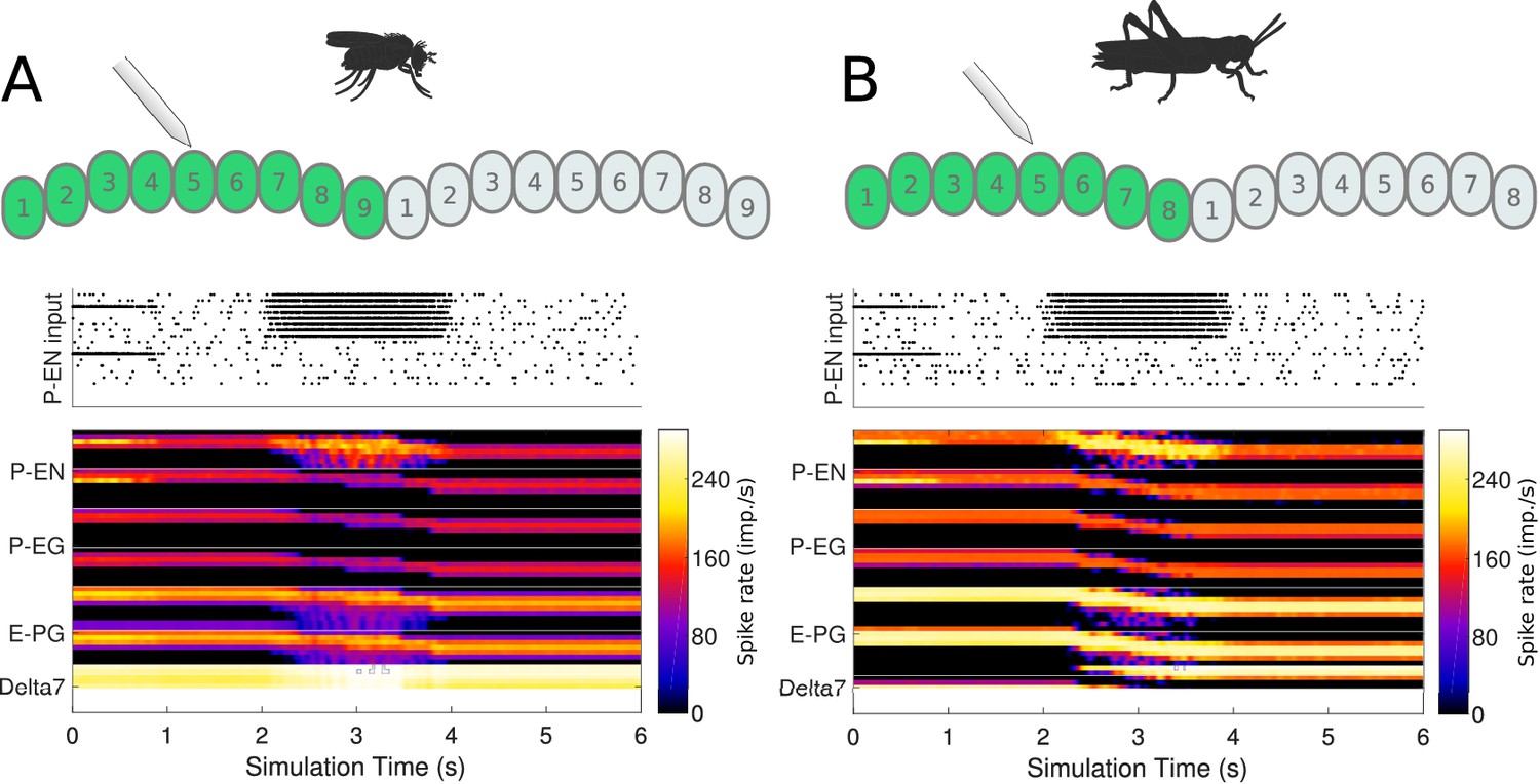
Response to uni-hemispheric stimulation.
Upper plots show the P-EN stimulation protocol and corresponding induced P-EN activity; lower plots show the response of the ring attractor for (A) the fruit fly circuit and (B) the locust circuit. The initial bilateral stimulation initialises a persistent activity ‘bump’, which moves around the circuit in response to stimulation of P-ENs in all the columns in one hemisphere only.
Figure 14
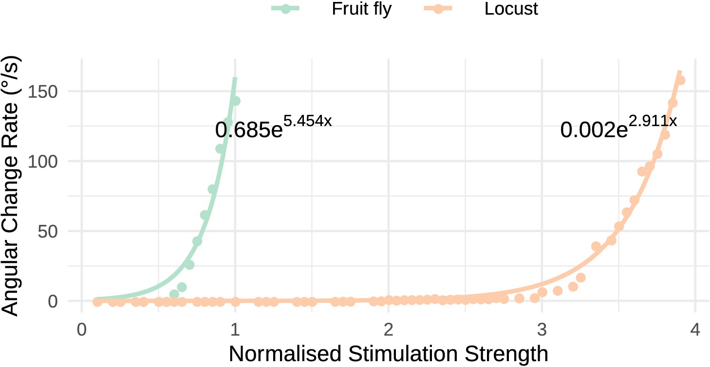
Response to uni-hemispheric stimulation.
Response rate of change of the heading signal with uni-hemispheric stimulation of P-EN neurons. The angular rate of change increases exponentially with stimulation strength and does so most rapidly for the fruit fly circuit. The data points have been fit with the function and the parameters of the fitted curves are shown on the plot.
Figure 15
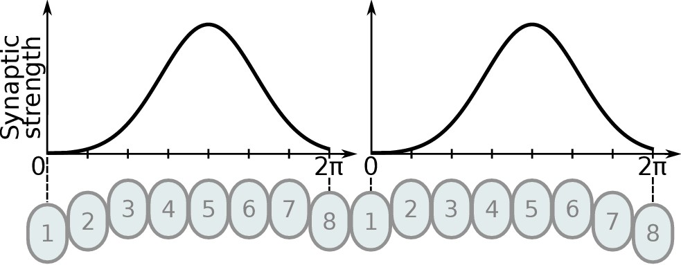
Illustration of Gaussian distribution of synaptic strengths.
The Gaussian distribution of synaptic strengths along synapses located in the PB glomeruli. The synaptic strengths along the PB are illustrated for one Delta7 neuron. The example illustrates the distribution for eight glomeruli, the same method is used for the hybrid-species model using nine glomeruli instead.
Figure 16
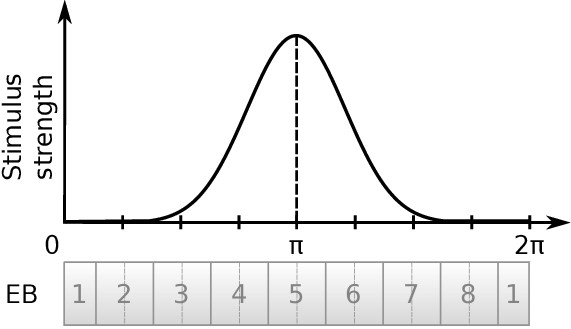
Illustration of von Mises distributed stimulus.
The curve demonstrates the relative intensity of the stimulus supplied to neurons innervating each EB tile. In this illustration the stimulus is centred at tile 5.
Tables
Table 1
Characteristics of the activity ‘bump’.
The Full Width at Half Maximum (FWHM), the peak impulse rate of the activity ‘bump’ formed across each family of neurons and the amplitude of the activity ‘bump’ measured as the range of firing rates are shown. Measurements were made 10 s after the stimulus was removed. Numbers are given as median and standard deviation. The activity of Delta7 neurons in Drosophila is approximately even, hence the corresponding FWHM measurement is not meaningful and marked as ‘N/A’.
| Neuron class | Drosophila | Locust | ||||
|---|---|---|---|---|---|---|
| FWHM | Peak | Amplitude | FWHM | Peak | Amplitude | |
(°)  | (imp./s)  | (imp./s) 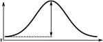 | (°)  | (imp./s)  | (imp./s) 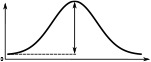 | |
| E-PG | 88.3 ± 0.3 | 161.0 ± 0.2 | 160.1 ± 0.3 | 68.3 ± 0.1 | 192.6 ± 0.1 | 192.0 ± 0.2 |
| P-EN | 80.4 ± 0.4 | 190.1 ± 0.2 | 190.1 ± 0.2 | 63.1 ± 0.3 | 153.5 ± 0.1 | 153.5 ± 0.1 |
| P-EG | 71.0 ± 0.2 | 190.1 ± 0.2 | 190.1 ± 0.2 | 63.1 ± 0.3 | 153.5 ± 0.1 | 153.5 ± 0.1 |
| Delta7 | N/A | 274.7 ± 0.1 | 27.1 ± 0.2 | 101.1 ± 0.2 | 266.6 ± 0.2 | 266.6 ± 0.2 |
Table 2
Characteristics of the neuron tuning curves.
The Full Width at Half Maximum (FWHM), the peak impulse rate of each family of neurons and the activity amplitude measured as the range of firing rates are shown. Numbers are given as median and standard deviation. The activity of Delta7 neurons in Drosophila is approximately even, hence the corresponding FWHM measurement is not meaningful and marked as ‘N/A’.
| Neuron class | Drosophila | Locust | ||||
|---|---|---|---|---|---|---|
| FWHM | Peak | Amplitude | FWHM | Peak | Amplitude | |
(°)  | (imp./s) 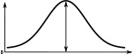 | (imp./s) 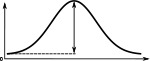 | (°)  | (imp./s)  | (imp./s) 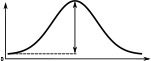 | |
| E-PG | 94.7 ± 4.0 | 208.4 ± 2.3 | 208.2 ± 2.2 | 73.4 ± 2.6 | 220.8 ± 1.4 | 220.8 ± 1.4 |
| P-EN | 74.6 ± 3.8 | 230.3 ± 2.3 | 230.3 ± 2.3 | 58.9 ± 3.1 | 163.6 ± 0.9 | 163.6 ± 0.9 |
| P-EG | 74.6 ± 3.8 | 230.3 ± 2.3 | 230.3 ± 2.3 | 58.9 ± 3.1 | 163.6 ± 0.9 | 163.6 ± 0.9 |
| Delta7 | N/A | 289.9 ± 1.8 | 58.1 ± 4.2 | 96.0 ± 3.2 | 265.4 ± 2.9 | 265.4 ± 2.9 |
Table 3
Neuronal nomenclature.
The names used for the homologous neurons differ between Drosophila and other species. The first column shows the name used in this paper to refer to each group of neurons. The other three columns provide the names used in the literature.
| Model | Drosophila | Locust | |
|---|---|---|---|
| Neuron name | Consensus name | Systematic name (Wolff and Rubin, 2018) | Name |
| E-PG | E-PG and E-PGT | PBG1-8.b-EBw.s-D/V GA.b and PBG9.b-EB.P.s-GA-t.b | CL1a |
| P-EN | P-EN | PBG2-9.s-EBt.b-NO1.b | CL2 |
| P-EG | P-EG | PBG1-9.s-EBt.b-D/V GA.b | CL1b |
| Delta7 | Delta7 or Δ7 | PB18.s-GxΔ7Gy.b and PB18.s-9i1i8c.b | TB1 |
Additional files
Download links
A two-part list of links to download the article, or parts of the article, in various formats.
Downloads (link to download the article as PDF)
Open citations (links to open the citations from this article in various online reference manager services)
Cite this article (links to download the citations from this article in formats compatible with various reference manager tools)
The head direction circuit of two insect species
eLife 9:e53985.
https://doi.org/10.7554/eLife.53985


