A decentralised neural model explaining optimal integration of navigational strategies in insects
- Computational Intelligence Lab & L-CAS, School of Computer Science, University of Lincoln, United Kingdom
- Machine Life and Intelligence Research Centre, Guangzhou University, China
- Sheffield Robotics, Department of Computer Science, University of Sheffield, United Kingdom
Figures
Figure 1

Overview of the unified navigation model and it’s homing capabilities.
(A) The homing behaviours to be produced by the model when displaced either from the nest and having no remaining PI home vector (zero vector), or from the nest with a full home vector (full vector). Distinct elemental behaviours are distinguished by coloured path segments, and stripped bands indicate periods where behavioural data suggests that multiple strategies are combined. Note that this colour coding of behaviour is maintained throughout the remaining figures to help the reader map function to brain region. (B) The proposed conceptual model of the insect navigation toolkit from sensory input to motor output. Three elemental guidance systems are modelled in this paper: path integration (PI), visual homing (VH) and route following (RF). Their outputs must then be coordinated in an optimal manner appropriate to the context before finally outputting steering command. (C) The unified navigation model maps the elemental guidance systems to distinct processing pathways: RF: OL - > AOTU - > BU - > CX; VH: OL - > MB - > SMP - > CX; PI: OL - > AOTU - > BU - > CX. The outputs are then optimally integrated in the proposed ring attractor networks of the FB in CX to generate a single motor steering command. Connections are shown only for the left brain hemisphere for ease of visualisation but in practice are mirrored on both hemispheres. Hypothesised or assumed pathways are indicated by dashed lines whereas neuroanatomically supported pathways are shown by solid lines (a convention maintained throughout all figures). OL: optic lobe, AOTU: anterior optic tubercle, CX: central complex, PB: protocerebrum bridge, FB: fan-shape body (or CBU: central body upper), EB: ellipsoid body (or CBL: central body lower), MB: mushroom body, SMP: superior medial protocerebrum, BU: bulb. Images of the brain regions are adapted from the insect brain database https://www.insectbraindb.org.
Figure 2
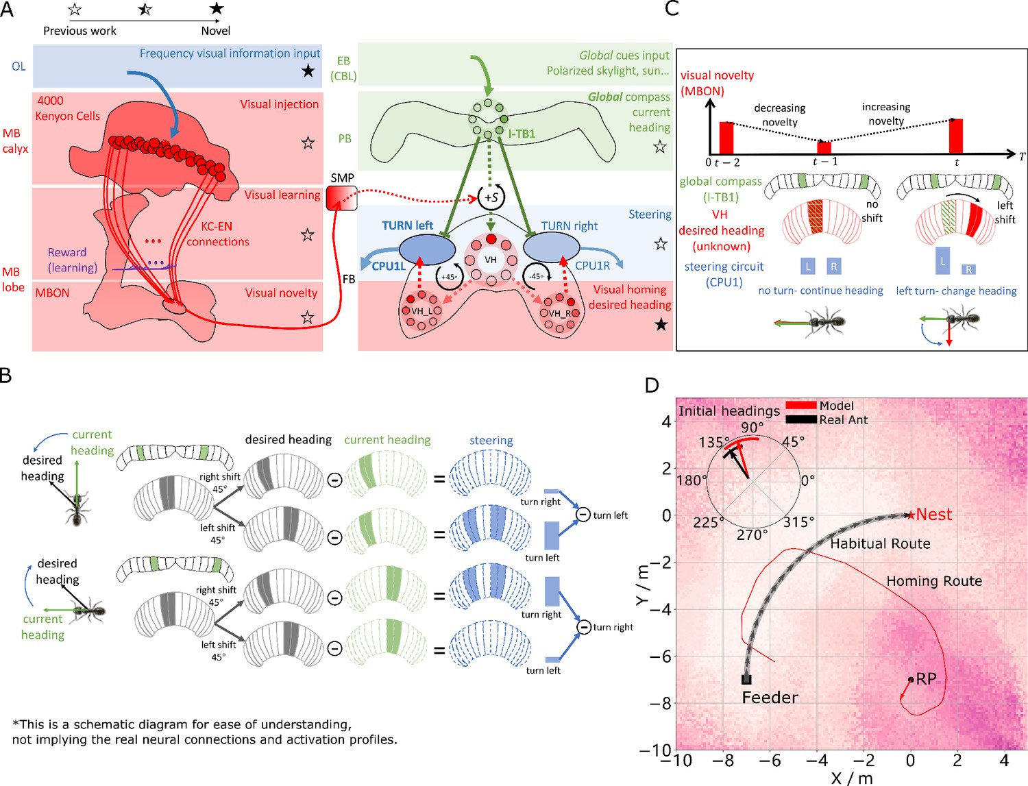
Visual homing in the insect brain.
(A) Neural model of visual homing. Rotational-invariant amplitudes are input to the MB calyx which are then projected to the Kenyon cells (KCs) before convergence onto the MB output neuron (MBON) which seeks to memorise the presented data via reinforcement-learning-based plasticity (for more details see Visual homing) (MB circuit: left panels). SMP neurons measure positive increases in visual novelty (through input from the MBON) which causes a shift between the current heading (green cells) and desired headings (red cells) in the rings of the CX (SMP pathway between MB and CX: centre panel; CX circuit: right panels). The CX-based steering circuit then computes the relevant turning angle. Example activity profiles are shown for an increase in visual novelty, causing a shift in desired heading and a command to change direction. Each model component in all figures is labelled with a shaded star to indicate what aspects are new versus those incorporated from previous models (see legend in upper left). (B) Schematic of the steering circuit function. First the summed differences between the impact of 45 °left and right turns on the desired heading and the current heading are computed. By comparing the difference between the resultant activity profiles allows an appropriate steering command to be generated. (C) Schematic of the visual homing model. When visual novelty drops ( to ) the desired heading is an unshifted copy of the current heading so the current path is maintained but when the visual novelty increases ( to ) the desired heading is shifted from the current heading. (D) The firing rate of the MBON sampled across locations at random orientations is depicted by the heat-map showing a clear gradient leading back to the route. The grey curve shows the habitual route along which ants were trained. RP (release point) indicates the position where real ants in Wystrach et al., 2012 were released after capture at the nest (thus zero-vector) and from which simulations were started. The ability of the VH model to generate realistic homing data is shown by the initial paths of simulated ants which closely match those of real ants (see inserted polar plot showing the mean direction and 95% confidential interval), and also the extended exampled path shown (red line). Note that once the agent arrives in the vicinity of the route, it appears to meander due the flattening of visual novelty gradient and the lack of directional information.
-
Figure 2—source data 1
The frequency information for the locations with random orientations across the world.
- https://cdn.elifesciences.org/articles/54026/elife-54026-fig2-data1-v2.mat
-
Figure 2—source data 2
The visual homing results of the model.
- https://cdn.elifesciences.org/articles/54026/elife-54026-fig2-data2-v2.mat
Figure 3 with 1 supplement
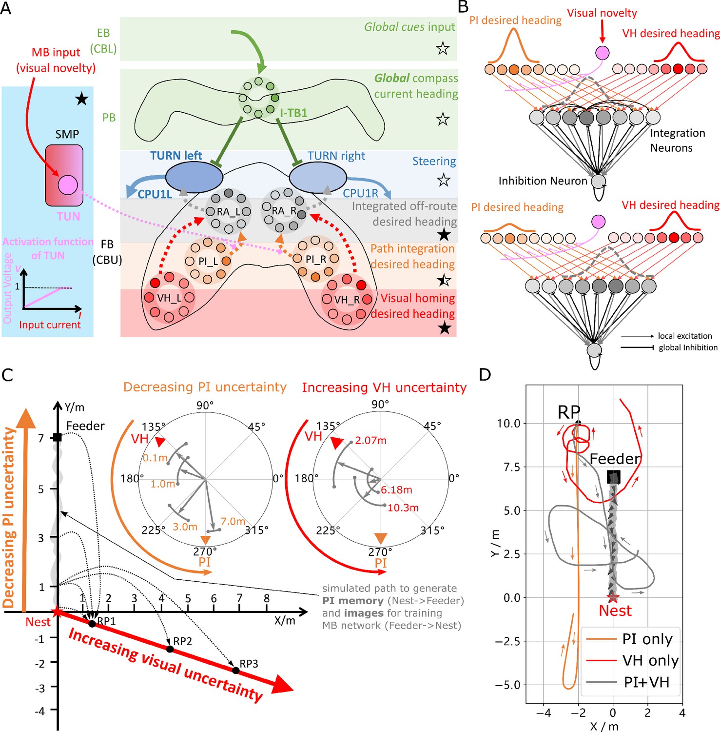
Optimal cue integration in the CX.
(A) Proposed model for optimally integrating PI and VH guidance systems. In each hemisphere, ring attractors (RAs) (grey neural rings) (speculatively located in FB/CBU) receive the corresponding inputs from PI (orange neural rings) and VH (red neural rings) with the outputs sent to the corresponding steering circuits (blue neural rings). Integration is weighted by the visual novelty tracking tuning neuron (TUN) whose activation function is shown in the leftmost panel. (B) Examples of optimal integration of PI and VH headings for two PI states with the peak stable state (grey dotted activity profile in the integration neurons) shifting towards VH as the home vector length recedes. (C) Replication of optimal integration studies of Wystrach et al., 2015 and Legge et al., 2014. Simulated ants are captured at various points (0.1 m, 1 m, 3 m and 7 m) along their familiar route (grey curve) and released at release point 1 (RP1) thus with the same visual certainty but with different PI certainties as in Wystrach et al., 2015 (see thick orange arrow). The left polar plot shows the initial headings of simulated ants increasingly weight their PI system (270°) in favour of their VH system (135°) as the home vector length increases and PI directional uncertainty drops. Simulated ants are also transferred from a single point 1 m along their familiar route to ever distant release points (RP1, RP2, RP3) thus with the same PI certainty but increasingly visual uncertainty as in Legge et al., 2014 (see thick red arrow). The right polar plot shows the initial headings of simulated ants increasingly weight PI (270°) over VH (135°) as visual certainty drops. (see Reproduce the optimal cue integration behaviour for details) (D) Example homing paths of the independent and combined guidance systems displaced from the familiar route (grey) to a fictive release point (RP).
-
Figure 3—source data 1
The results of tuning PI uncertainty.
- https://cdn.elifesciences.org/articles/54026/elife-54026-fig3-data1-v2.zip
-
Figure 3—source data 2
The results of tuning VH uncertainty.
- https://cdn.elifesciences.org/articles/54026/elife-54026-fig3-data2-v2.zip
-
Figure 3—source data 3
The extended homing path of PI, VH and combined PI and VH.
- https://cdn.elifesciences.org/articles/54026/elife-54026-fig3-data3-v2.zip
Figure 3—figure supplement 1
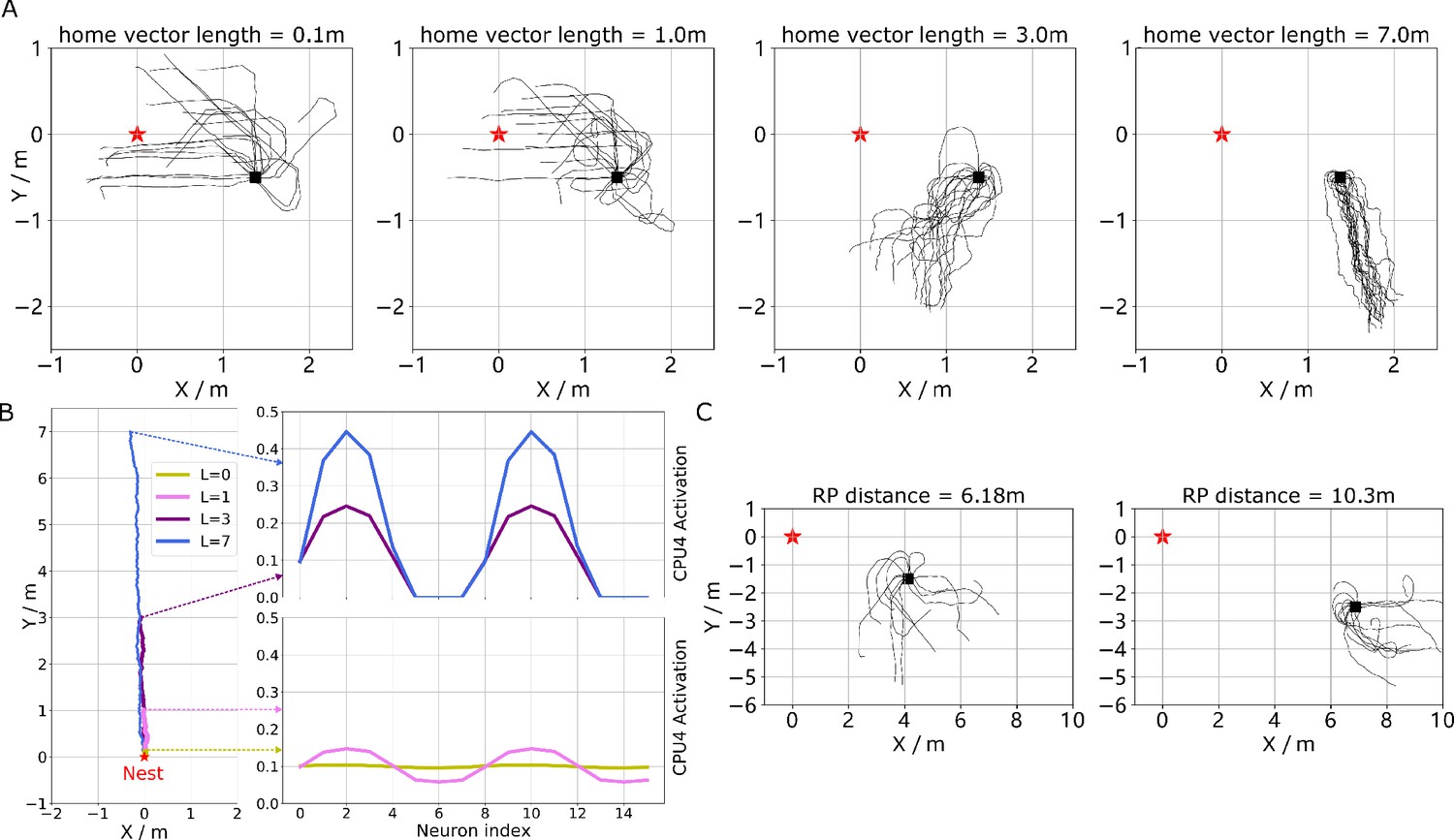
The extended homing paths and the PI memory in the simulations.
Figure 4
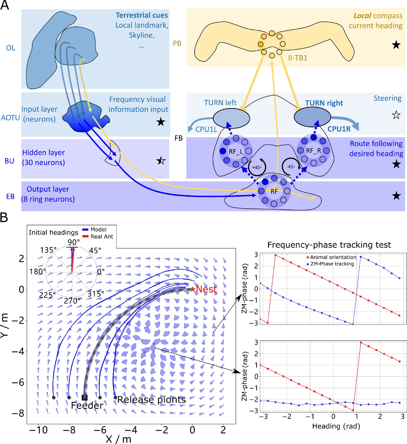
Phase-based route following.
(A) Neural model. The visual pathway from the optic lobe via AOTU and Bulb to EB of the CX is modelled by a fully connected artificial neural network (ANN) with one hidden layer. The input layer receives the amplitudes of the frequency encoded views (as for the MB network) and the output layer is an 8-neuron ring whose population encoding represents the desired heading against to which the agent should align. (B) Behaviours. Blue and red arrows in the inserted polar plot (top left) display the mean directions and 95% confidential intervals of the initial headings of real (Wystrach et al., 2012) and simulated ants released at the start of the route , respectively. Dark blue curves show the routes followed by the model when released at five locations close to the start of the learned path. The overlaid fan-plots indicate the circular statistics (the mean direction and 95% confidential interval) of the homing directions recommended by the model when sampled across heading directions (20 samples at 18°intervals). Data for entire rotations are shown on the right for specific locations with the upper plot, sampled at , demonstrating accurate phase-based tracking of orientation, whereas the lower plot sampled at shows poor tracking performance and hence produces a wide fan-plot.
-
Figure 4—source data 1
The frequency tracking performance across the world.
- https://cdn.elifesciences.org/articles/54026/elife-54026-fig4-data1-v2.mat
-
Figure 4—source data 2
The RF model results of the agents released on route.
- https://cdn.elifesciences.org/articles/54026/elife-54026-fig4-data2-v2.mat
-
Figure 4—source data 3
The RF model results of the agents released aside from the route.
- https://cdn.elifesciences.org/articles/54026/elife-54026-fig4-data3-v2.mat
Figure 5
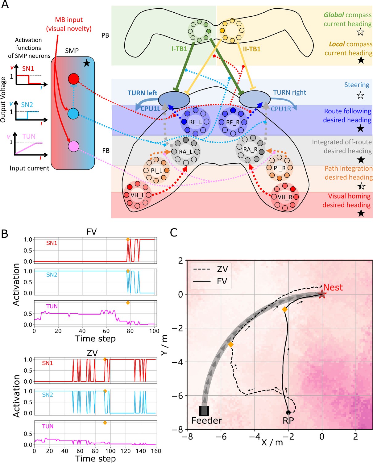
Unified model realising the full array of coordinated navigational behaviours.
(A) Context-dependent switching is realised using two switching neurons (SN1, SN2) that have mutually exclusive firing states (one active while the other is in active) allowing coordination between On and Off-Route strategies driven by the instantaneous visual novelty output by the MB. Connectivity and activation functions of the SMP neurons are shown in the left side of panel. (B) Activation history of the SN1, SN2 and TUN (to demonstrate the instantaneous visual novelty readout of the MB) neurons during the simulated displacement trials. (C) Paths generated by the unified model under control of the context-dependent switch circuit during simulated FV (solid line) and ZV (dashed line) displacement trials.
-
Figure 5—source data 1
The navigation results of the whole model.
- https://cdn.elifesciences.org/articles/54026/elife-54026-fig5-data1-v2.zip
Figure 6
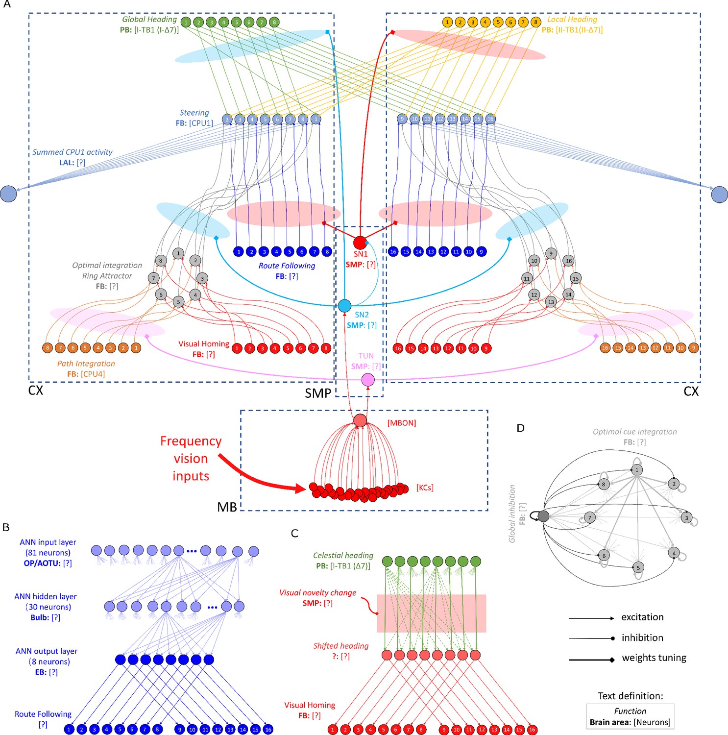
The detailed neural connections of the proposed model.
(A): The detailed neural connections of the navigation coordination system. (B): The neural connection of the route following network. The input layer to the hidden layer is fully connected, so does the hidden layer to the output layer. (C): The network generating the visual homing memory. (D): The detailed neural connection of the ring attractor network for optimal cue integration.
Figure 7
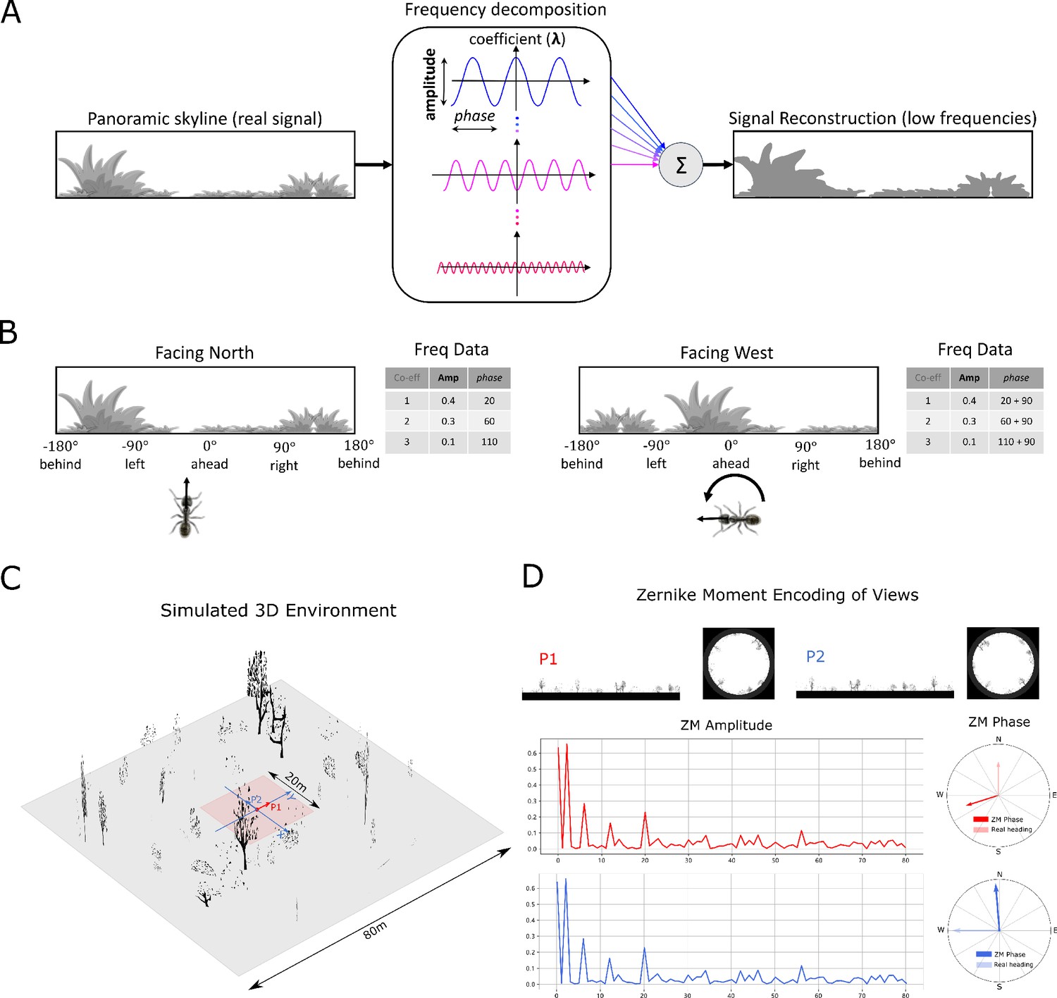
Information provided by frequency encoding in cartoon and simulated ant environments.
(A): A cartoon depiction of a panoramic skyline, it’s decomposition into trigonometric functions, and reconstruction through the summation of low frequency coefficients reflecting standard image compression techniques. (B): Following a 90° rotation there is no change in the amplitudes of the frequency coefficients but the phases of the frequency coefficients track the change in orientation providing a rotational invariant signal useful for visual homing and rotationally-varying signal useful for route following, respectively. (C): The simulated 3D world used for all experiments. The pink area (size: ) is used for model training and testing zone for models allowing obstacle-free movement. (D): The frequency encoding (Zernike Moment’s amplitudes and phase) of the views sampled from the same location but with different headings (P1 and P2 in (C), with heading difference) in the simulated world. The first 81 amplitudes are identical while the phases have the difference of about .
-
Figure 7—source data 1
The matrix of simulated 3D world.
- https://cdn.elifesciences.org/articles/54026/elife-54026-fig7-data1-v2.mat
Tables
Table 1
The detailed parameters settings for the simulations.
| Para. | Visual homing | Optimal integration tuning PI | Optimal integration tuning VH | Route following | Whole model ZV | Whole model FV |
|---|---|---|---|---|---|---|
| (Equation 14) | 0.04 | 0.04 | 0.04 | 0.04 | 0.04 | 0.04 |
| (Equation 16) | 0.1 | 0.1 | 0.1 | 0.1 | 0.1 | 0.1 |
| (Equation 19) | 2.0 | 2.0 | 2.0 | / | 0.5 | 0.5 |
| (Equation 28) | / | 0.1 | 0.1 | / | 0.025 | 0.0125 |
| (Equation 32) | / | / | / | / | 2.0 | 3.0 |
| (Equation 35) | 0.125 | 0.125 | 0.125 | 0.125 | 0.375 | 0.375 |
| (cm/step) (Equation 39) | 4 | 4 | 4 | 4 | 8 | 8 |
| initial heading (deg) | 0~360 | 0~360 | 0~360 | 0 / 180 | 90 | 0 |
Table 2
The details of the main neurons used in the proposed model.
| Name | Function | Num | Network | Brain region | Neuron in species(e.g.) | Reference |
|---|---|---|---|---|---|---|
| I-TB1 | Global compasscurrent heading | 8 | Ring attractor | CX | TB1 in Schistocerca gregariaand Megalopta genalis | Heinze and Homberg, 2008; Stone et al., 2017 |
| II-TB1 | Local compasscurrent heading | 8 | Ring attractor | Δ7 in Drosophila | Franconville et al., 2018 | |
| S I-TB1 | Copy of shiftedglobal heading | 8 | Ring | No data | / | |
| VH-L | VH desiredheading left | 8 | Ring | No data | ||
| VH-R | VH desiredheading right | 8 | Ring | No data | ||
| PI-L | PI desiredheading left | 8 | Ring | CPU4 in Schistocerca gregariaand Megalopta genalis | Heinze and Homberg, 2008; Stone et al., 2017 | |
| PI-R | PI desiredheading right | 8 | Ring | P-F3N2v in Drosophila | Franconville et al., 2018 | |
| RF-L | RF desiredheading left | 8 | Ring | No data | / | |
| RF-R | RF desiredheading right | 8 | Ring | No data | ||
| RA-L | Cue integrationleft | 8 | Ring attractor | No data | ||
| RA-R | Cue integrationright | 8 | Ring attractor | No data | ||
| CPU1 | Comparing thecurrent anddesired heading | 16 | Steering circuit | CPU1 in Schistocerca gregaria and Megalopta genalis PF-LCre in Drosophila | Heinze and Homberg, 2008; Stone et al., 2017Franconville et al., 2018 | |
| vPN | visual projection | 81 | Associative learning | MB | MB neurons in Drosophila | Aso et al., 2014 |
| KCs | Kenyon cells | 4000 | Camponotus | Ehmer and Gronenberg, 2004 | ||
| MBON | visual novelty | 1 | Apis mellifera | Rybak and Menzel, 1993 | ||
| TUN | Tuning weightsfrom PI to RA | 1 | / | SMP | No data | / |
| SN1 | Turn on/off theRF output to CPU1 | 1 | Switch circuit | No data | ||
| SN2 | Turn on/off theRA output to CPU1 | 1 | Switch circuit | No data |
Additional files
-
Source code 1
Data_Model_Simulations_Results.
- https://cdn.elifesciences.org/articles/54026/elife-54026-code1-v2.zip
-
Transparent reporting form
- https://cdn.elifesciences.org/articles/54026/elife-54026-transrepform-v2.docx
Download links
A two-part list of links to download the article, or parts of the article, in various formats.
Downloads (link to download the article as PDF)
Open citations (links to open the citations from this article in various online reference manager services)
Cite this article (links to download the citations from this article in formats compatible with various reference manager tools)
A decentralised neural model explaining optimal integration of navigational strategies in insects
eLife 9:e54026.
https://doi.org/10.7554/eLife.54026


