Control of adaptive action selection by secondary motor cortex during flexible visual categorization
Figures
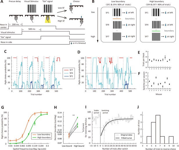
Flexible visual categorization task.
(A) Schematic of the task and timing of behavioral events. (B) Visual stimuli and categorical boundaries. Each session consisted of alternating low-boundary and high-boundary blocks, the order of which was counterbalanced across sessions. For low-boundary blocks, SF1 and SF4 were presented for 90% of trials; for high-boundary blocks, SF4 and SF7 were presented for 90% of trials. (C and D) Performance of one example mouse for SF1 (0.03 cycles/o), SF4 (0.095 cycles/o) and SF7 (0.3 cycles/o) in two different sessions. For each trial, the probability of right choice was computed over the previous 15 trials. H, high-boundary block; L, low-boundary block. (E) Number of trials per block for each mouse. (F) Number of switches per session for each mouse. (G) Psychometric curves from low-boundary and high-boundary blocks for an example mouse (data from 11 sessions). (H) Comparison of internal decision boundary between blocks for a population of mice. p=2 × 10⁻³, n = 10 mice, Wilcoxon signed rank test. (I) Performance for the reversing stimulus before and after the boundary switch for an example mouse. The curve is an exponential fit of the data after the boundary switch. (J) Distribution of the number of trials to reverse choice, which was the number of trials for the correct rate of reversing stimulus to reach 50% after the boundary switch. n = 10 mice. Error bar,± SEM. See Figure 1—source data 1–2 for complete statistics.
-
Figure 1—source data 1
Number of trials per block, number of switches per session and number of trials to reverse choice for a population of mice.
- https://cdn.elifesciences.org/articles/54474/elife-54474-fig1-data1-v2.txt
-
Figure 1—source data 2
Psychometric curves and decision boundary for low-boundary and high-boundary blocks.
- https://cdn.elifesciences.org/articles/54474/elife-54474-fig1-data2-v2.txt
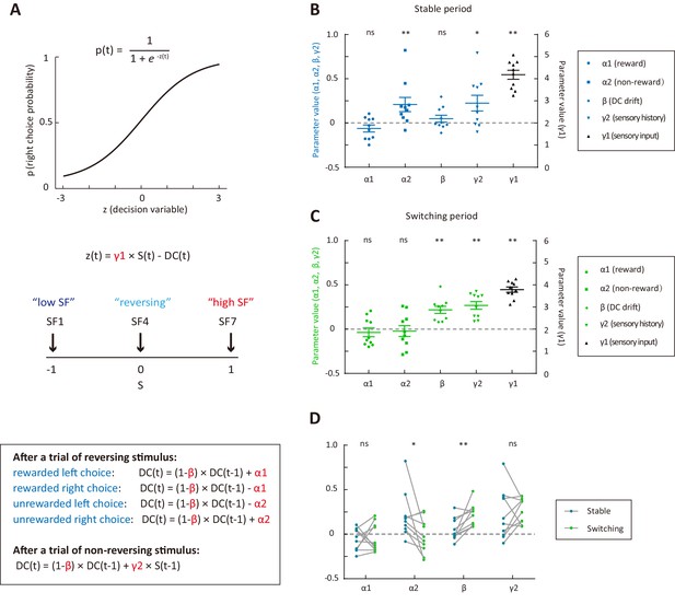
Behavioral strategies revealed by computational modelling.
(A) Schematic of the dynamic DC model, in which the DC was updated on a trial-by-trial basis according to choice outcome history (α1 and α2) or sensory history (γ2). (B) Model parameters for the stable period. (C) Model parameters for the switching period. (D) Comparison of parameters important for the update of DC between the stable and the switching periods. *p<0.05, **p<0.01, n = 10 mice, Wilcoxon signed rank test. See Figure 2—source data 1 for complete statistics.
-
Figure 2—source data 1
Parameters of the dynamic-DC model fitted to choices in the stable and switching periods separately.
- https://cdn.elifesciences.org/articles/54474/elife-54474-fig2-data1-v2.txt
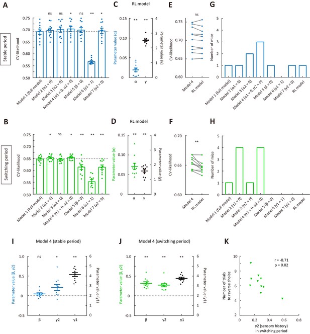
Comparison of cross-validated likelihood among different models.
(A) CV likelihood of different variants of the dynamic-DC model for the stable period. For each of the reduced model variants (model 2 – model 7), we compared the CV likelihood with that of the full model. Dashed line, the CV likelihood averaged across 10 mice for the full model. (B) CV likelihood of different variants of the dynamic-DC model for the switching period. Similar to that described in (A). (C) Parameters of the RL model for the stable period. (D) Parameters of the RL model for the switching period. (E) Comparison of CV likelihood between the RL model and model 4 of the dynamic-DC model for the stable period. p=0.32, Wilcoxon signed rank test. (F) Comparison of CV likelihood between the RL model and model 4 of the dynamic-DC model for the switching period. p=2 × 10⁻³, Wilcoxon signed rank test. (G) Best model frequency (number of mice a model being the best model) for each model in the stable period. (H) Best model frequency for each model in the switching period. (I) Parameters of model four in the stable period. (J) Parameters of model four in the switching period. (K) Correlation between sensory history parameter γ2 (model 4) in the switching period and the number of trials to reverse choice. *p<0.05, **p<0.01, n = 10 mice, Wilcoxon signed rank test. Error bar,± SEM. For more details, see Figure 3—figure supplements 1–7. See Figure 3—source data 1–3 for complete statistics.
-
Figure 3—source data 1
Cross-validated likelihood for each model.
- https://cdn.elifesciences.org/articles/54474/elife-54474-fig3-data1-v2.txt
-
Figure 3—source data 2
Parameter values for model 4.
- https://cdn.elifesciences.org/articles/54474/elife-54474-fig3-data2-v2.txt
-
Figure 3—source data 3
Parameter values for the RL model.
- https://cdn.elifesciences.org/articles/54474/elife-54474-fig3-data3-v2.txt
-
Figure 3—source data 4
Comparison of cross-validated likelihood among different models that were fitted to data in all trials.
- https://cdn.elifesciences.org/articles/54474/elife-54474-fig3-data4-v2.txt
-
Figure 3—source data 5
Visualization of the simulated behavior for model 1 and model 4.
- https://cdn.elifesciences.org/articles/54474/elife-54474-fig3-data5-v2.txt
-
Figure 3—source data 6
Parameter recovery analysis.
- https://cdn.elifesciences.org/articles/54474/elife-54474-fig3-data6-v2.txt
-
Figure 3—source data 7
Right choice bias for reversing stimulus under two different conditions of sensory history.
- https://cdn.elifesciences.org/articles/54474/elife-54474-fig3-data7-v2.txt
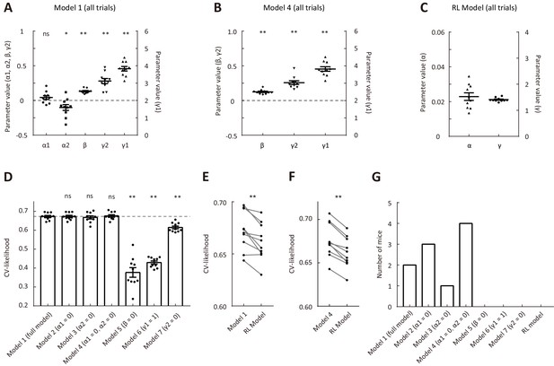
Comparison of cross-validated likelihood among different models that were fitted to data in all trials.
(A) Parameters of model 1. (B) Parameters of model 4. (C) Parameters of the RL model. (D) CV likelihood of different variants of the dynamic-DC model. For each of the reduced model variants (model 2 – model 7), we compared the CV likelihood with that of the full model. Dashed line, the CV likelihood averaged across 10 mice for the full model. (E) Comparison of CV likelihood between the RL model and model 1 of the dynamic-DC model. p=0.004, Wilcoxon signed rank test. (F) Comparison of CV likelihood between the RL model and model 4 of the dynamic-DC model. p=0.002, Wilcoxon signed rank test. (G) Best model frequency (number of mice a model being the best model) for each model. *p<0.05, **p<0.01, n = 10 mice, Wilcoxon signed rank test. Error bar,± SEM. See Figure 3—source data 4 for complete statistics.
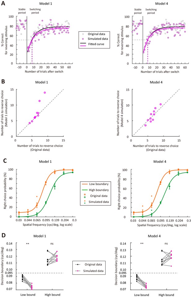
Model simulation for model 1 and model four using the parameters of the model fitted to data in all trials.
(A) Simulated performance for the reversing stimulus in trials before and after the boundary switch for model 1 (left) and model 4 (right), using the model parameters of an example mouse. (B) Comparison of the number of trials to reverse choice between the simulated data and the actual data (n = 10 mice). Left, model one was simulated. Right, model four was simulated. (C) Simulated psychometric curves for model 1 (left) and model 4 (right), using the model parameters of an example mouse. The orange and green curves are curve fits for the original data. (D) Comparison of the decision boundary between the simulated data and the actual data (n = 10 mice). Left, model one was simulated. Right, model four was simulated. **p<0.01, Wilcoxon signed rank test. See Figure 3—source data 5 for complete statistics.
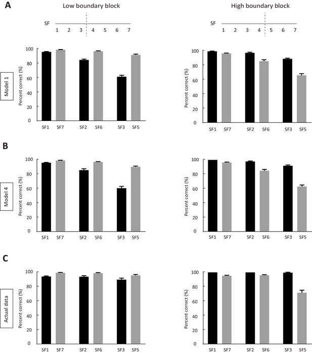
Simulated and actual performance for stimuli at SFs lower or higher than the SF of reversing stimulus.
(A) Performance of simulated data produced by model 1, using model parameters of the 10 mice in Figure 1. Left, low-boundary block. Right, high-boundary block. SF4 indicates the reversing stimulus. SF1 and SF7 indicate the lowest and the highest SF, respectively. (B) Performance of simulated data produced by model 4, using model parameters of the 10 mice in Figure 1. Left, low-boundary block. Right, high-boundary block. (C) Actual performance for the 10 mice in Figure 1. Left, low-boundary block. Right, high-boundary block. See Figure 3—source data 5 for complete statistics.
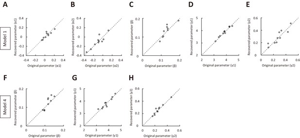
Parameter recovery for model 1 and model 4, using parameters of the model fitted to data in all trials.
(A–E) Parameter recovery for α1, α2, β, γ1 and γ2 in model 1. (F–H) Parameter recovery for β, γ1 and γ2 in model 4. The original parameters were from model 1 (or model 4) fitted to data in all trials for the 10 mice in Figure 1. Values along the identity line indicate good agreement between simulated and original parameters. See Figure 3—source data 6 for complete statistics.
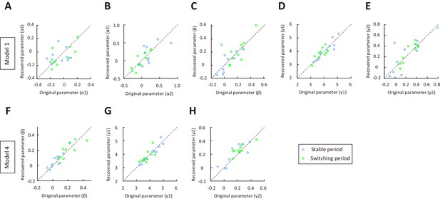
Parameter recovery for model 1 and model 4, using parameters of the model fitted separately to choices in switching and stable periods.
(A–E) Parameter recovery for α1, α2, β, γ1 and γ2 in model 1. Blue, stable period. Green switching period. (F–H) Parameter recovery for β, γ1 and γ2 in model 4. The original parameters were from model 1 (or model 4) fitted separately to choices in switching and stable periods for the 10 mice in Figure 1. Values along the identity line indicate good agreement between recovered and original parameters. See Figure 3—source data 6 for complete statistics.
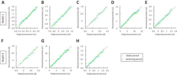
Parameter recovery for model 1 and model 4, using a wide range of model parameters for the switching and stable periods.
(A–E) Parameter recovery for α1, α2, β, γ1 and γ2 in model 1. Blue, stable period. Green switching period. (F–H) Parameter recovery for β, γ1 and γ2 in model 4. Values along the identity line indicate good agreement between recovered and original parameters. See Figure 3—source data 6 for complete statistics.
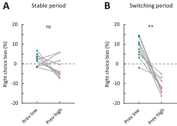
Comparison of right choice bias between two types of sensory history.
(A) Right choice bias in the stable period. (B) Right choice bias in the switching period. Prev low, low-frequency stimulus in the previous trial (i.e., previous-trial SF was lower than the reversing stimulus SF). Prev high, high-frequency stimulus in the previous trial (i.e., previous-trial SF was higher than the reversing stimulus SF). **p<0.01, n = 10 mice, Wilcoxon signed rank test. See Figure 3—source data 7 for complete statistics.
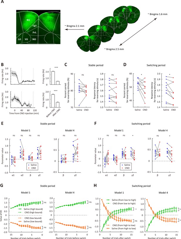
Bilateral inactivation of M2 impairs adaptive action selection in the switching period.
(A) Representative fluorescence images showing the expression of AAV2/9-hSyn-hM4D-mCitrine in M2. (B) Firing rates of M2 neurons before and after CNO injection. Upper row, firing rates for 24 neurons recorded from one mouse (bar plot, mean firing rates 0–20 min before and 40–120 min after CNO injection). Lower row, firing rates for 14 neurons recorded from another mouse (bar plot, mean firing rates 0–20 min before and 40–100 min after CNO injection). The two vertical dashed lines indicate the time points corresponding to the start and end of a behavioral session, respectively. (C) Comparison of performance in the stable period between saline and CNO sessions. Left, correct rate for the reversing stimulus; right, response latency for the reversing stimulus. (D) Comparison of performance in the switching period between saline and CNO sessions, similar to that described in (C). (E) Parameters of the dynamic-DC model in the stable period. Left, model 1; right, model 4 (α1 = 0 and α2 = 0). (F) Parameters of the dynamic-DC model in the switching period. Left, model 1; right, model 4. (G) Comparison of DC curves in the stable period between saline and CNO sessions. Left, model 1; right, model 4. (H) Comparison of DC curves in the switching period between saline and CNO sessions. Left, model 1; right, model 4. *p<0.05, ***p<0.001. Wilcoxon signed rank test for (B). Two-way repeated measures ANOVA followed by Sidak’s multiple comparisons test for (C and D). Two-way repeated measures ANOVA for (G and H). Data in (C−H) were from n = 10 mice. Shading and error bar,± SEM. For more details of the effect of chemogenetic manipulation, see Figure 4—figure supplements 1–7. See Figure 4—source data 1–5 for complete statistics.
-
Figure 4—source data 1
Effect of M2 inactivation on behavioral performance and model parameters.
- https://cdn.elifesciences.org/articles/54474/elife-54474-fig4-data1-v2.txt
-
Figure 4—source data 2
Performance and model parameters for control mice with EGFP expressed in M2.
- https://cdn.elifesciences.org/articles/54474/elife-54474-fig4-data2-v2.txt
-
Figure 4—source data 3
Parameter recovery analysis for saline and CNO sessions of M2 inactivation.
- https://cdn.elifesciences.org/articles/54474/elife-54474-fig4-data3-v2.txt
-
Figure 4—source data 4
Effect of mPFC inactivation on behavioral performance and model parameters.
- https://cdn.elifesciences.org/articles/54474/elife-54474-fig4-data4-v2.txt
-
Figure 4—source data 5
Effect of OFC inactivation on behavioral performance and model parameters.
- https://cdn.elifesciences.org/articles/54474/elife-54474-fig4-data5-v2.txt

Effect of M2 inactivation on behavioral performance.
(A and B) Performance for the reversing stimulus before and after boundary switch for two example mice. The curves are exponential fit of the data after the boundary switch. Blue, saline sessions. Red, CNO sessions. (C) Psychometric curves averaged over all mice (n = 10) for low- and high-boundary blocks, respectively. Solid curves, saline sessions. Dashed curves, CNO sessions.
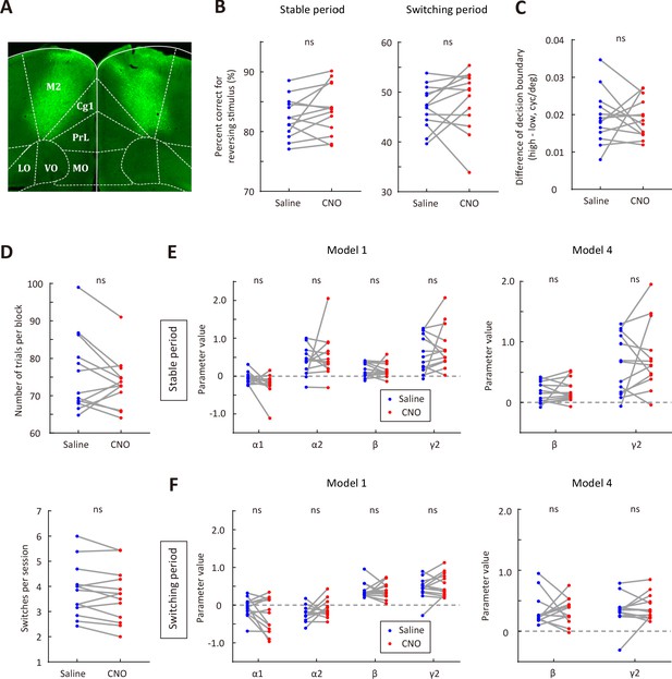
Effect of CNO injection on the performance of EGFP-expressing control mice.
(A) Representative fluorescence image showing the expression of AAV2/8-CamKIIa-EGFP-3Flag-WPRE-SV40pA in M2. (B) Correct rate for the reversing stimulus in saline vs CNO sessions. Left, stable period; right, switching period. (C) The difference of decision boundary in saline vs CNO sessions. (D) Upper, number of trials per block in saline vs CNO sessions. Lower, number of switches per session in saline vs CNO sessions. (E) Comparison of model parameters in the stable period between saline and CNO sessions. Left, full model; right, model 4 (α1 = 0 and α2 = 0). (F) Comparison of model parameters in the switching period between saline and CNO sessions. Left, full model; right, model 4. n = 13 mice, Wilcoxon signed rank test. See Figure 4—source data 2 for complete statistics.

M2 inactivation did not affect the performance for non-reversing stimuli (A), number of trials per block (B), number of switches per session (C) or the distance between internal decision boundaries (D).
n = 10 mice, Wilcoxon signed rank test. See Figure 4—source data 1 for complete statistics.
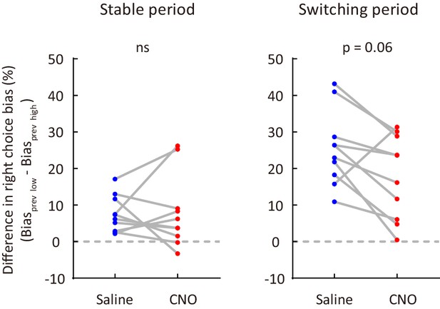
Effect of M2 inactivation on sensory history-dependent right choice bias.
To compute the difference in right choice bias, the right choice bias for a previous low-frequency stimulus was subtracted by the right choice bias for a previous high-frequency stimulus. n = 10 mice, Wilcoxon signed rank test. See Figure 4—source data 1 for complete statistics.
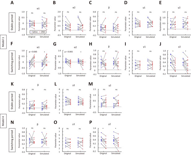
Parameter recovery for model 1 and model 4, using parameters of the model fitted separately to data in saline sessions and in CNO sessions.
(A–E) Original and recovered parameters of model one for the stable period. Blue, saline sessions. Red, CNO sessions. (F–J) Original and recovered parameters of model one for the switching period. (K–M) Original and recovered parameters of model four for the stable period. (N–P) Original and recovered parameters of model four for the switching period. *p<0.05, n = 10 mice, Wilcoxon signed rank test. See Figure 4—source data 3 for complete statistics.
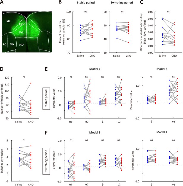
Effect of mPFC inactivation on behavioral performance.
(A) Representative fluorescence image showing the expression of AAV2/9-hSyn-hM4D-mCitrine in mPFC. (B) Comparison of correct rate for the reversing stimulus between saline and CNO sessions. Left, stable period; right, switching period. (C) The difference of decision boundary in saline vs CNO sessions. (D) Upper, number of trials per block in saline vs CNO sessions. Lower, number of switches per session in saline vs CNO sessions. (E) Comparison of model parameters in the stable period between saline and CNO sessions. Left, model 1; right, model 4. (F) Comparison of model parameters in the switching period between saline and CNO sessions. Left, model 1; right, model 4. n = 13 mice. Wilcoxon signed rank test. See Figure 4—source data 4 for complete statistics.
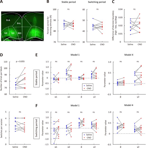
Effect of OFC inactivation on behavioral performance.
(A) Representative fluorescence image showing the expression of AAV2/9-hSyn-hM4D-mCitrine in OFC. (B) Comparison of correct rate for the reversing stimulus between saline and CNO sessions. Left, stable period; right, switching period. (C) The difference of decision boundary in saline vs CNO sessions. (D) Upper, number of trials per block in saline vs CNO sessions. Lower, number of switches per session in saline vs CNO sessions. (E) Comparison of model parameters in the stable period between saline and CNO sessions. Left, model 1; right, model 4. (F) Comparison of model parameters in the switching period between saline and CNO sessions. Left, model 1; right, model 4. n = 9 mice. Wilcoxon signed rank test. See Figure 4—source data 5 for complete statistics.
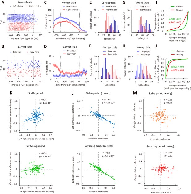
Correlation between choice preference and previous-stimulus preference for M2 neurons.
(A) Spike raters of an example M2 neuron in 20 reversing-stimulus trials, grouped by left or right choice. The two vertical dashed lines indicate the time of stimulus onset and ‘Go’ signal onset, respectively. (B) Spike raters of another example M2 neuron in 20 reversing-stimulus trials, grouped by previous stimulus (previous low or previous high SF). (C) PSTHs of the M2 neuron in (A) in correct reversing-stimulus trials, grouped by left or right choice. (D) PSTHs of the M2 neuron in (B) in correct reversing-stimulus trials, grouped by previous stimulus (previous low or previous high SF). (E) Frequency histogram of left-choice and right-choice responses from the M2 neuron in (A) in correct trials. (F) Frequency histogram of previous-low-frequency and previous-high-frequency responses from the M2 neuron in (B) in correct trials. (G) Frequency histogram of left-choice and right-choice responses from the M2 neuron in (A) in wrong trials. (H) Frequency histogram of previous-low-frequency and previous-high-frequency responses from the M2 neuron in (B) in wrong trials. (I) ROC curves for the two pairs of response distributions illustrated in (E) and (G), respectively. (J) ROC curves for the two pairs of response distributions illustrated in (F) and (H), respectively. (K) Left-right choice preference in correct and wrong trials was significantly correlated. n = 113 neurons. Upper, stable period; lower, switching period. (L) Left-right choice preference and previous-stimulus preference were significantly correlated in correct trials. n = 72 neurons. Upper, stable period; lower, switching period. (M) Left-right choice preference and previous-stimulus preference were not significantly correlated in wrong trials. n = 72 neurons. Upper, stable period; lower, switching period. r, Pearson’s correlation coefficient. Shading in (C and D), ± SEM. See Figure 5—figure supplements 1–7 for more details of the recording and data analysis. See Figure 5—source data 1 for complete statistics.
-
Figure 5—source data 1
Choice preference and previous-stimulus preference for M2 neurons.
- https://cdn.elifesciences.org/articles/54474/elife-54474-fig5-data1-v2.txt
-
Figure 5—source data 2
Model parameters and right choice bias for the mice used for electrophysiologcial recordings.
- https://cdn.elifesciences.org/articles/54474/elife-54474-fig5-data2-v2.txt
-
Figure 5—source data 3
Choice preference and previous-stimulus preference for M2 neurons recorded from the left and right hemispheres, respectively.
- https://cdn.elifesciences.org/articles/54474/elife-54474-fig5-data3-v2.txt
-
Figure 5—source data 4
Sliding window analysis of the correlation between choice preference and previous-stimulus preference of M2 neurons in correct trials.
- https://cdn.elifesciences.org/articles/54474/elife-54474-fig5-data4-v2.txt
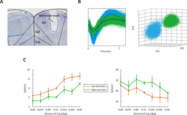
Electrophysiological recordings from M2.
(A) Verification of M2 recording site. Arrow shows electrolytic lesion made after the final recording session. (B) Left, example of spike waveforms. Right, single units were identified using cluster analysis of principle component amplitudes. (C) Responses of two example M2 neurons to different SFs. See Figure 5—source data 1 for complete statistics.
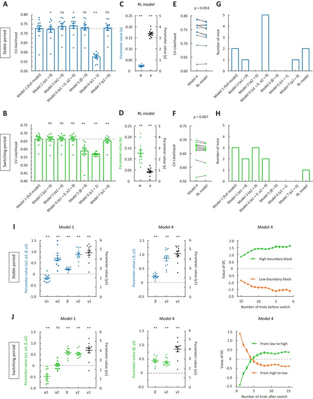
Model fitting for the behavioral data of mice used for electrophysiological recordings.
(A) CV likelihood of different variants of the dynamic-DC model for the stable period. For each of the reduced model variants (model 2 – model 7), we compared the CV likelihood with that of the full model. Dashed line, the CV likelihood averaged across 11 mice for the full model. (B) CV likelihood of different variants of the dynamic-DC model for the switching period. Similar to that described in (A). (C) Parameters of the RL model for the stable period. (D) Parameters of the RL model for the switching period. (E) Comparison of the CV likelihood between the RL model and model 4 of the dynamic-DC model for the stable period. (F) Comparison of the CV likelihood between the RL model and model 4 of the dynamic-DC model for the switching period. (G) Best model frequency (number of mice a model being the best model) for each model in the stable period. (H) Best model frequency for each model in the switching period. (I) Left and middle, parameters of the dynamic-DC model (model 1 and model 4) in the stable period. Right, curve of DC value (model 4) in the stable period. (J) Left and middle, parameters of the dynamic-DC model (model 1 and model 4) in the switching period. Right, curve of DC value (model 4) in the switching period. *p<0.05, **p<0.01, n = 11 mice, Wilcoxon signed rank test. Error bar,± SEM. See Figure 5—source data 2 for complete statistics.
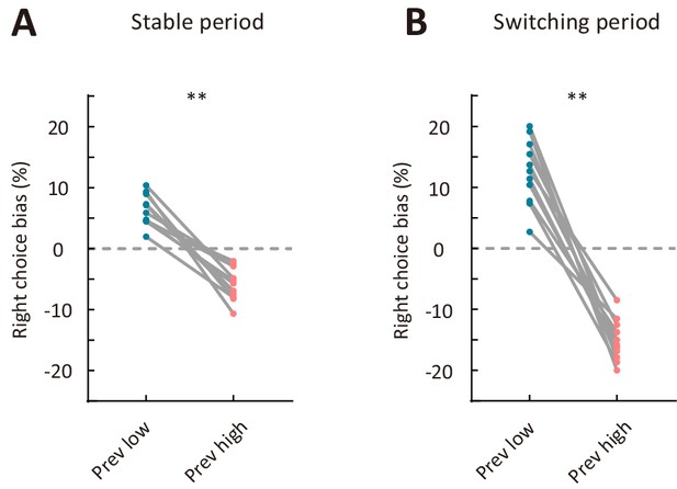
Comparison of right choice bias between two types of sensory history for mice used for electrophysiological recordings.
(A) Right choice bias in the stable period. (B) Right choice bias in the switching period. Prev low, low-frequency stimulus in the previous trial (i.e., previous-trial SF was lower than the reversing stimulus SF). Prev high, high-frequency stimulus in the previous trial (i.e., previous-trial SF was higher than the reversing stimulus SF). **p<0.01, n = 11 mice, Wilcoxon signed rank test. See Figure 5—source data 2 for complete statistics.
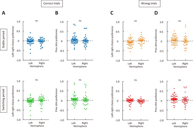
Choice preference and previous-stimulus preference for M2 neurons recorded from the left and right hemispheres.
(A) Left-right choice preference in correct trials. Upper, stable period; lower, switching period. (B) Previous-stimulus preference in correct trials. Upper, stable period; lower, switching period. (C) Left-right choice preference in wrong trials. Upper, stable period; lower, switching period. (D) Previous-stimulus preference in wrong trials. Upper, stable period; lower, switching period. Left hemisphere, n = 44 neurons; right hemisphere, n = 28 neurons. Wilcoxon rank sum test. See Figure 5—source data 3 for complete statistics.
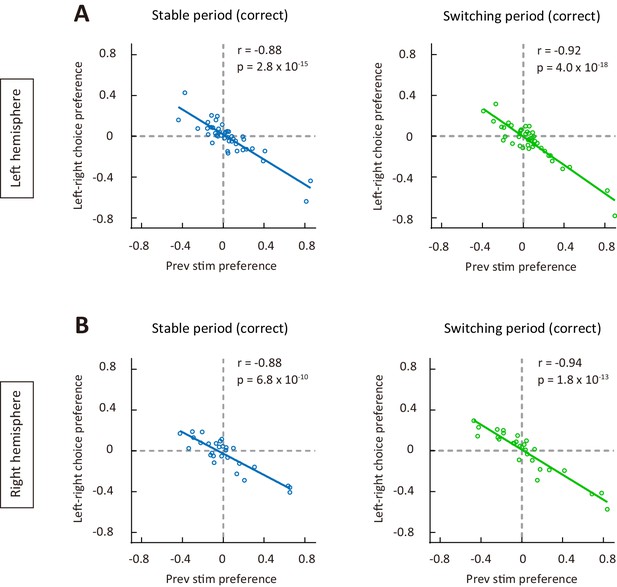
The correlation between choice preference and previous-stimulus preference in correct trials for M2 neurons in left and right hemispheres, respectively.
(A) Left-right choice preference and previous-stimulus preference were significantly correlated in correct trials for n = 44 neurons from left hemisphere. Left, stable period; right, switching period. (B) Left-right choice preference and previous-stimulus preference were significantly correlated in correct trials for n = 28 neurons from right hemisphere. Left, stable period; right, switching period. r, Pearson’s correlation coefficient. See Figure 5—source data 3 for complete statistics.
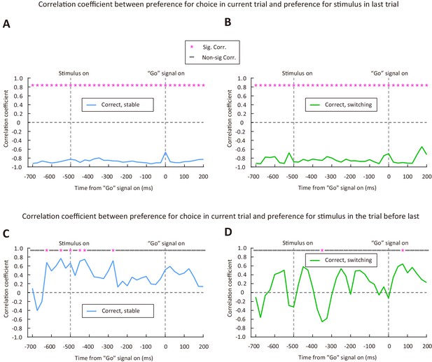
Sliding window analysis of the correlation between choice preference and previous-stimulus preference for correct trials.
(A and B) Correlation coefficient between the preference for choice in current trial and the preference for stimulus in last trial. (A) Stable period. (B) Switching period. n = 72 neurons. (C and D) Correlation coefficient between the preference for choice in current trial and the preference for stimulus in the trial before last. (C) Stable period. (D) Switching period. Time 0 is the time of “Go” signal onset, and -700 ms is the time of central port entry. * marks the time bins with significant correlation coefficient (p < 0.05). See Figure 5—source data 4 for complete statistics.
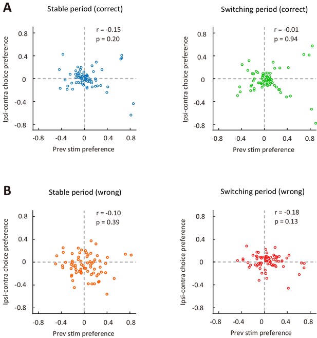
Choice preference (ipsilateral vs contralateral) was not significantly correlated with preference for previous stimulus (low-frequency vs high-frequency) for M2 neurons.
(A) Correct trials in the stable period (left) and the switching period (right). (B) Wrong trials in the stable period (left) and the switching period (right). The ipsilateral-contralateral choice preference was computed using the responses of ipsilateral and contralateral choices. n = 72 neurons. r, Pearson’s correlation coefficient. See Figure 5—source data 1 for complete statistics.
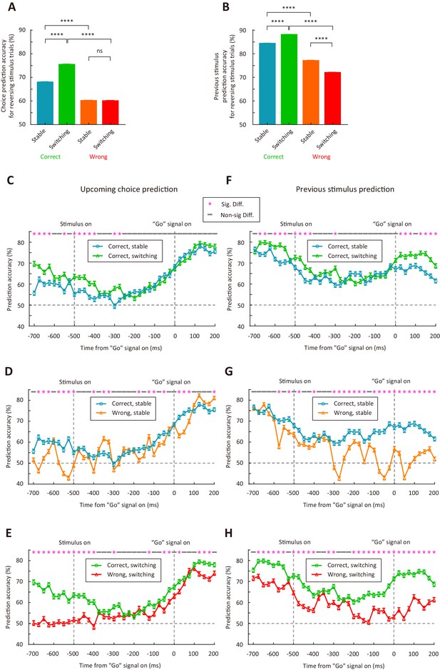
M2 neurons encode upcoming choice and previous stimulus more accurately in the switching than in the stable period.
(A) Prediction accuracy for upcoming choice in response to the reversing stimulus. n = 1500 resampled datasets, 113 neurons. (B) Prediction accuracy for stimulus in previous trial. n = 1500 resampled datasets, 72 neurons. (C–H) Temporal dynamics of decoding accuracy. Time 0 is the time of ‘Go’ signal onset, and −700 ms is the time of central port entry. (C−E) Prediction accuracy for upcoming choice in response to the reversing stimulus. (F−H) Prediction accuracy for stimulus in previous trial. For (A and B), ****, p<1.0 × 10⁻⁴, Wilcoxon rank sum test. For (C–H), * marks the time bins with p<0.05, two-way ANOVA followed by Sidak’s multiple comparisons test. See Figure 6—source data 1 for complete statistics.
-
Figure 6—source data 1
SVM analysis of M2 activity.
- https://cdn.elifesciences.org/articles/54474/elife-54474-fig6-data1-v2.txt
Tables
| Reagent type (species) or resource | Designation | Source or reference | Identifiers | Additional information |
|---|---|---|---|---|
| Strain, strain background Mus musculus | C67BL/6 | Slac Laboratory Animal | N/A | |
| Chemical compound, drug | clozapine-N-Oxide | Sigma-Aldrich Corporation | C0832-5MG | |
| Software, algorithm | Offline Sorter | Plexon | https://plexon.com | |
| Software, algorithm | Prism | GraphPad | https://www.graphpad.com/scientificsoftware/prism/; RRID:SCR_00279 | |
| Software, algorithm | MATLAB | Mathworks | https://www. mathworks.com/;RRID:SCR_001622 |


