Vestigial auriculomotor activity indicates the direction of auditory attention in humans
- Systems Neuroscience and Neurotechnology Unit, Faculty of Medicine, Saarland University & School of Engineering, htw saar, Germany
- Audiological Research Unit, Sivantos GmbH, Germany
- Clinical and Cognitive Neuroscience Laboratory, Department of Psychological Sciences, University of Missouri, United States
Figures
Figure 1

Experimental setup.
(A) Four loudspeakers presented novel sounds (Exp. 1) or stories (Exp. 2) at 30° to the left or right of fixation or behind the interaural axis. Instructions, text, or fixation cross was displayed on a 55 in flat screen. (B) Surface EMGs were recorded bilaterally from four auricular muscles as well as from left zygomaticus major, frontalis, and sternocleidomastoideus, using a bandpass of 10 – 1000 Hz and a sampling rate of 9600 Hz. Separation of paired auricular electrodes was 1 cm.
Figure 2 with 1 supplement
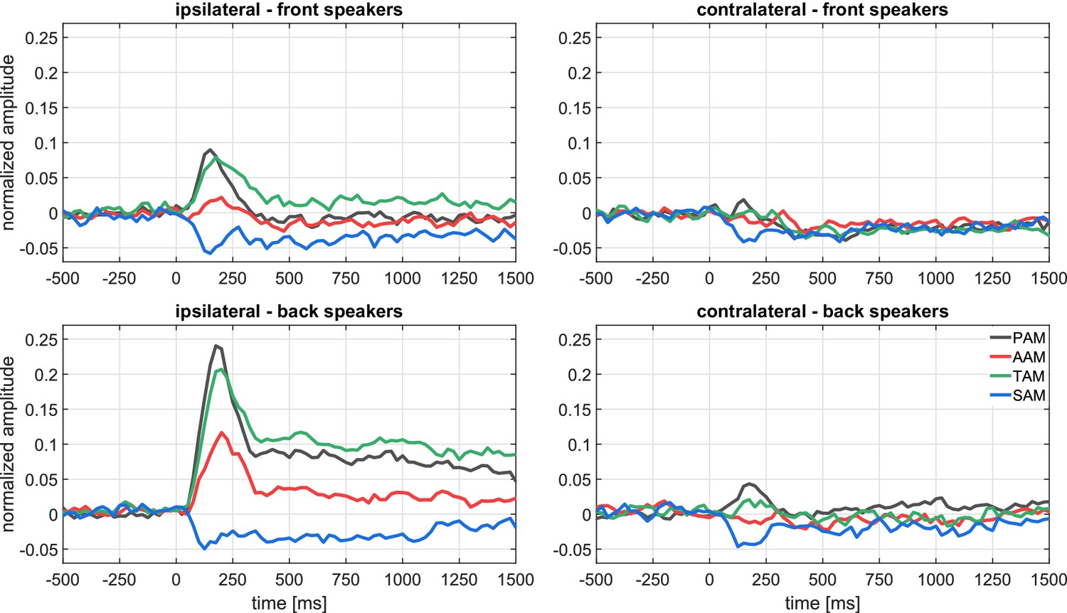
Experiment 1.
Grand average (N = 28) of the baseline corrected and normalized event-related electromyograms at the four auricular muscles for the recordings ipsilateral (left panel) and contralateral (right panel) to stimulation; top: front speakers (30°), bottom: back speakers (120°). The contralateral-ipsilateral organization of our data set is justified by a preliminary analysis that obtained null effects for left–versus–right using a more complete factorial structure (left/right stimulus direction × left/right recording site). The following figure supplement is available for Figure 2—figure supplement 1. Analysis of video recordings from one participant who exhibited submillimeter pinna displacements in response to stimulation from the back speakers. This figure supplement is complemented by Video 1 and Video 2.
Figure 2—figure supplement 1
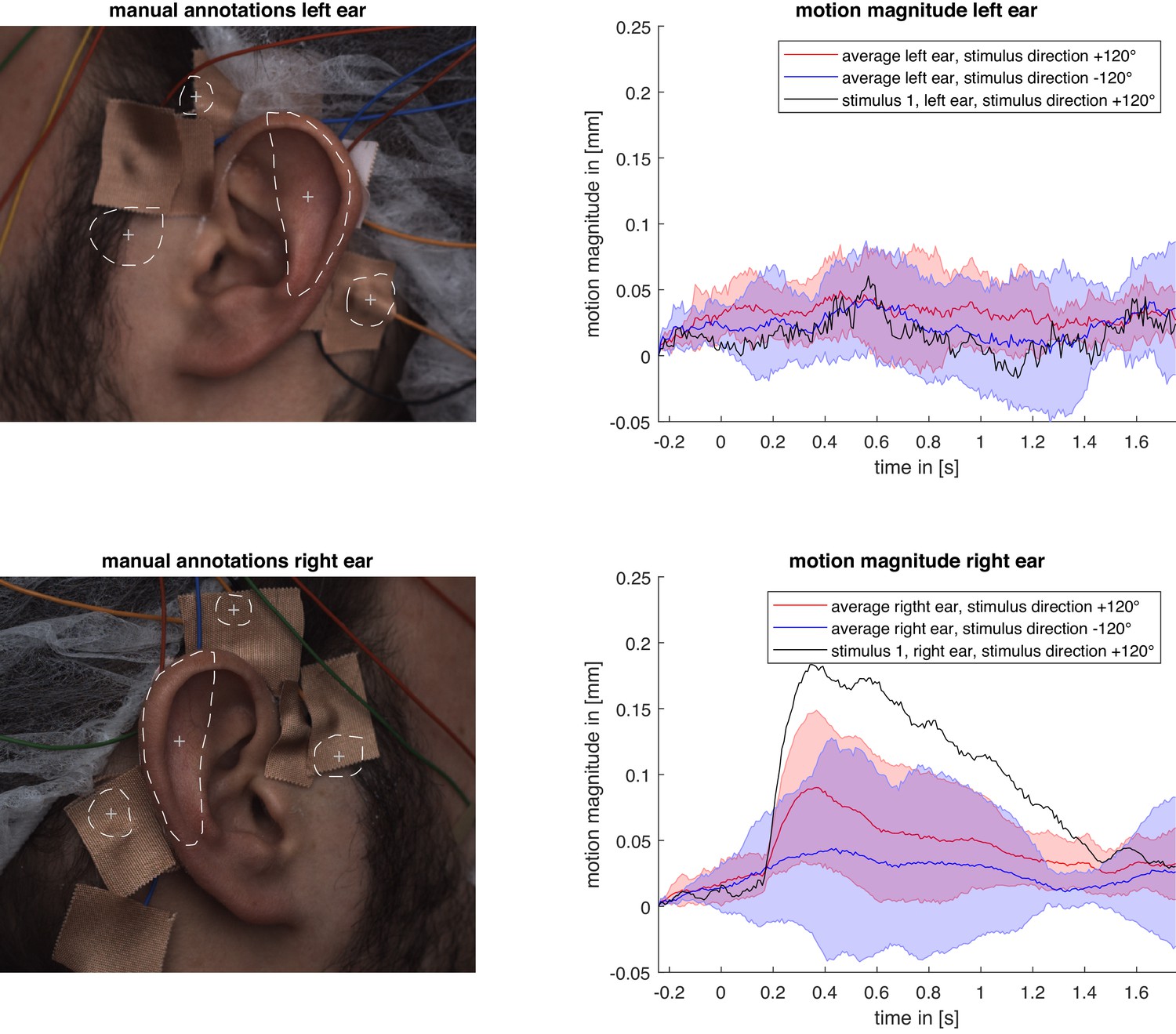
Analysis of video recordings from one participant who exhibited submillimeter pinna displacements in response to stimulation in Experiment 1 (Exogenous Attention).
Given the time of a stimulus, we analyzed 2s video segments with pre-stimulus onset . The frames at of the first stimulus (direction +120°) of the left and right recordings were manually annotated with four regions of interest (ROI) (left images). The centroid of the ROI located on the ear was used to track the pinna motion and the three centroids of the ROIs around the ears were used to define a basis of a coordinate system where the coordinates of points on the ear are invariant under head motion. Each point inside the ROIs sampled as in the first frame was projected to the respective right camera frames and forward-warped with respect to the motion to the reference frame for all cameras. The motion magnitude is given as the norm of at time with respect to the basis referenced to at . On the right are the time courses of the mean motion magnitude and standard deviation over the stimuli (± 120°) for the left and the right ear as well as the time course of the first stimulus from the right back speaker. This is the same trial that is portrayed in Video 1 and Video 2. Due to a large head rotation during the recording, the first − 120° stimulus was excluded from the evaluation.
Figure 3 with 3 supplements
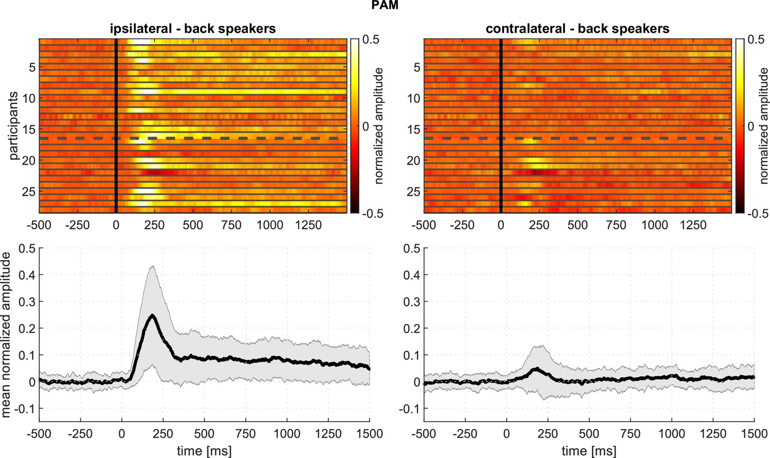
Experiment 1 – Responses of the PAM to stimuli from the back speakers, showing intersubject variability: Top panels: Every row corresponds to the averaged response of one participant.
Amplitude is encoded in color. The top rows (1-16) represent younger adult participants; the bottom rows (17-28), older adults. Bottom panels: Mean and standard deviation based on the above plots. The following figure supplements are available for Figure 3—figure supplement 1. The described intersubject variability analysis for the AAM, Figure 3—figure supplement 2. SAM, and Figure 3—figure supplement 3. TAM.
Figure 3—figure supplement 1
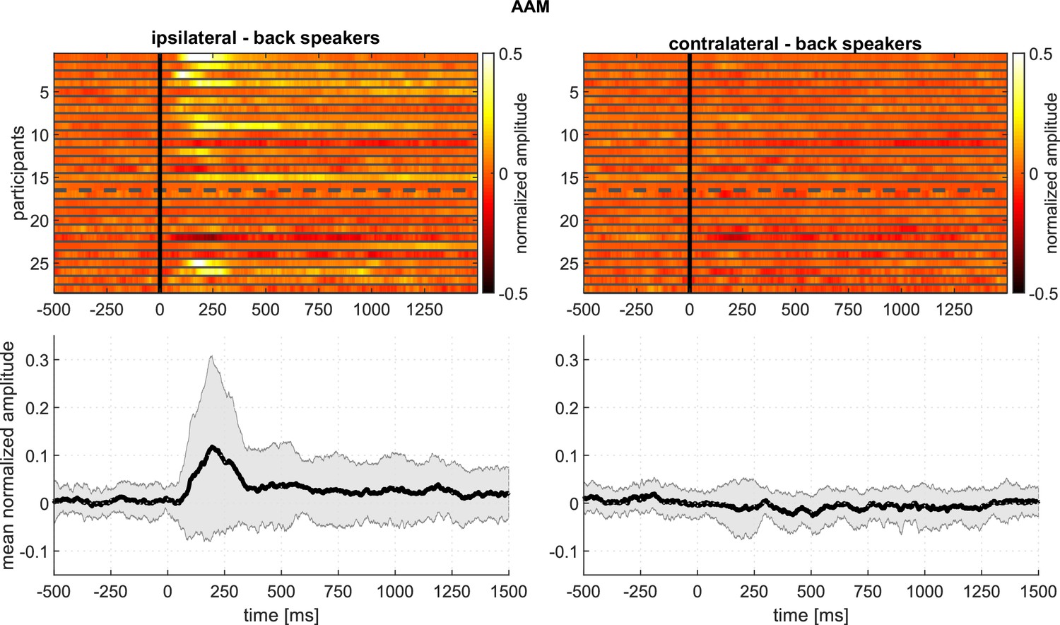
Experiment 1 – Responses of the AAM to stimuli from the back speakers, showing intersubject variability: Top panels: Every row corresponds to the averaged response of one participant.
Amplitude is encoded in color. The top rows (1-16) represent younger adult participants; the bottom rows (17-28), older adults. Bottom panels: Mean and standard deviation based on the above plots.
Figure 3—figure supplement 2
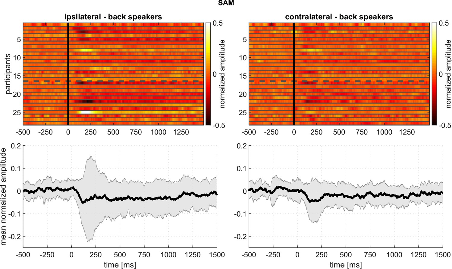
Experiment 1 – Responses of the SAM to stimuli from the back speakers, showing intersubject variability: Top panels: Every row corresponds to the averaged response of one participant.
Amplitude is encoded in color. The top rows (1-16) represent younger adult participants; the bottom rows (17-28), older adults. Bottom panels: Mean and standard deviation based on the above plots.
Figure 3—figure supplement 3
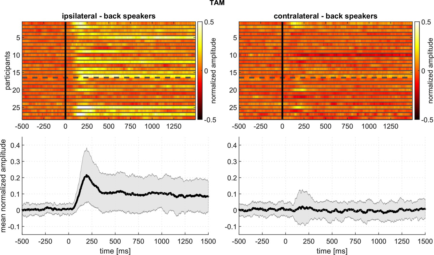
Experiment 1 – Responses of the TAM to stimuli from the back speakers, showing intersubject variability: Top panels: Every row corresponds to the averaged response of one participant.
Amplitude is encoded in color. The top rows (1-16) represent younger adult participants; the bottom rows (17-28), older adults. Bottom panels: Mean and standard deviation based on the above plots.
Figure 4 with 3 supplements
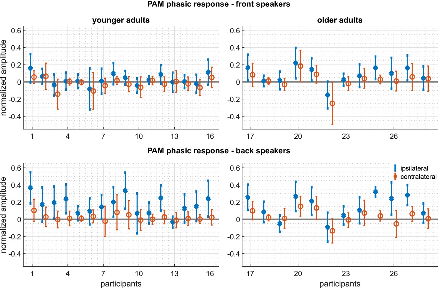
Experiment 1 – Intrasubject variability of the PAM: Mean and standard deviations of the phasic responses 50 - 300 ms) of every participant.
Top panels: responses to the front speakers. Bottom panels: responses to the back speakers. Left panels: Responses of the younger adults. Right panels: responses of the older adults. Blue represents ipsilateral responses, red represents contralateral responses. The following figure supplements are available for Figure 4—figure supplement 1. The described intrasubject variability analysis for the AAM, Figure 4—figure supplement 2. SAM, and Figure 4—figure supplement 3. TAM.
Figure 4—figure supplement 1
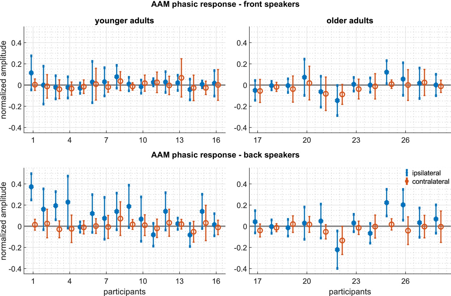
Experiment 1 – Intrasubject variability of the AAM: Mean and standard deviations of the phasic responses ( 50 - 300 ms) of every participant.
Top panels: responses to the front speakers. Bottom panels: responses to the back speakers. Left panels: Responses of the younger adults. Right panels: responses of the older adults. Blue represents ipsilateral responses, that is EMG recorded from the muscle on the same side as the stimulus, whereas red represents contralateral responses.
Figure 4—figure supplement 2
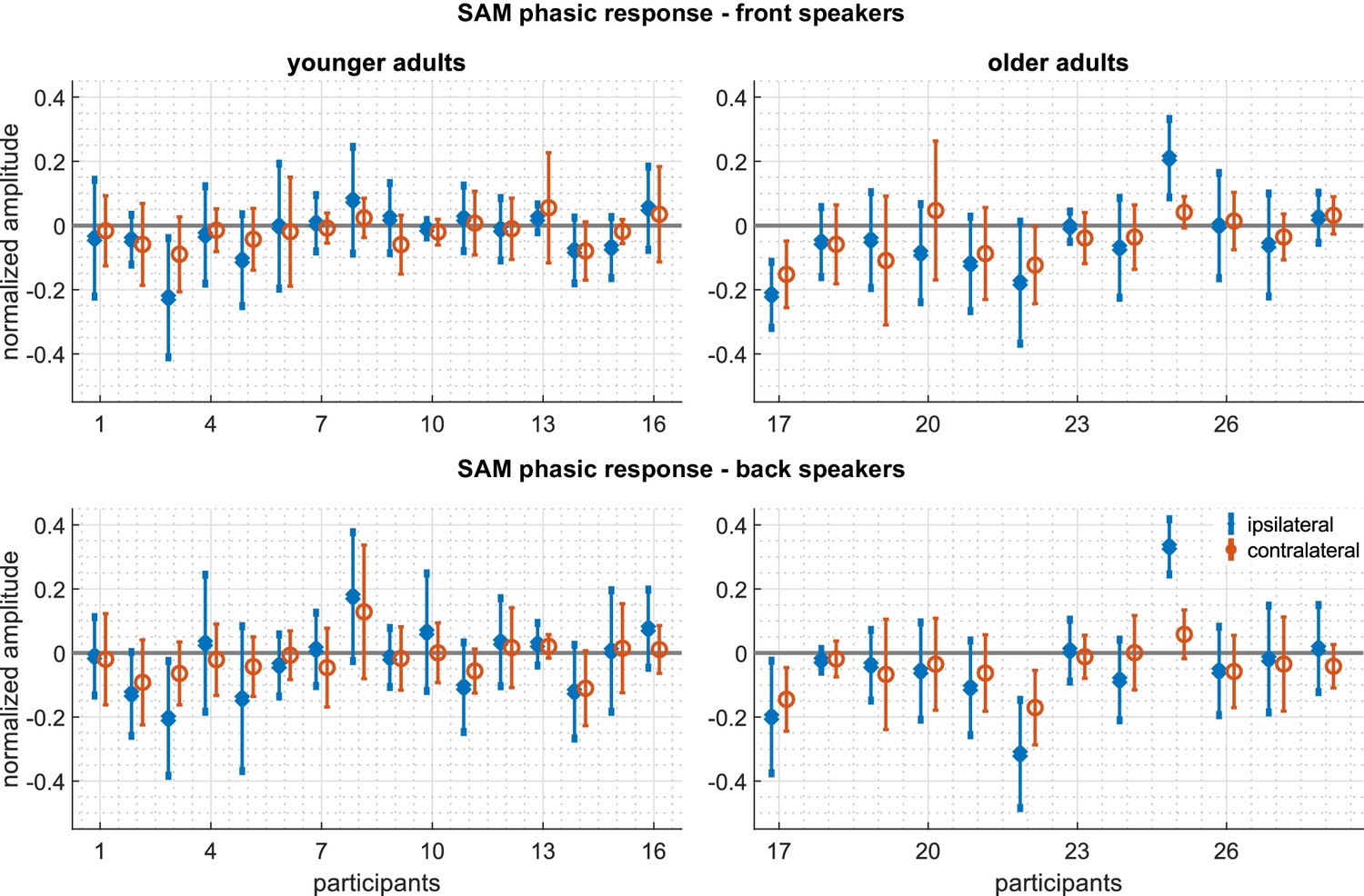
Experiment 1 – Intrasubject variability of the SAM: Mean and standard deviations of the phasic responses (50 -300 ms) of every participant.
Top panels: responses to the front speakers. Bottom panels: responses to the back speakers. Left panels: Responses of the younger adults. Right panels: responses of the older adults. Blue represents ipsilateral responses, that is EMG recorded from the muscle on the same side as the stimulus, whereas red represents contralateral responses.
Figure 4—figure supplement 3
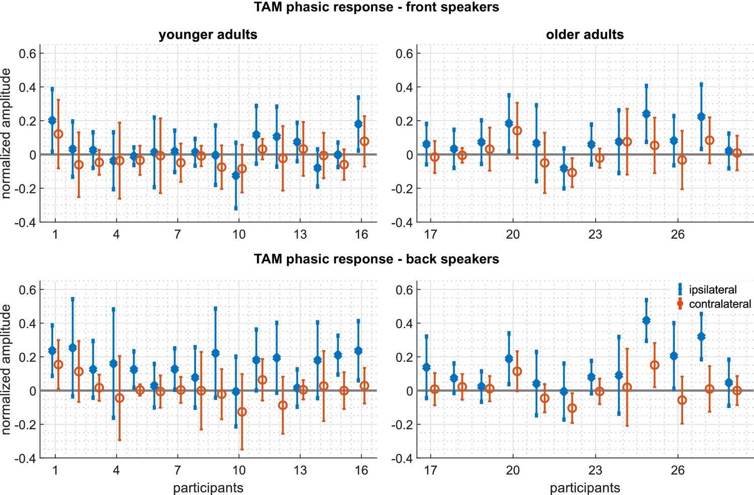
Experiment 1 – Intrasubject variability of the TAM: Mean and standard deviations of the phasic responses ( 50 - 300 ms) of every participant.
Top panels: responses to the front speakers. Bottom panels: responses to the back speakers. Left panels: Responses of the younger adults. Right panels: responses of the older adults. Blue represents ipsilateral responses, that is EMG recorded from the muscle on the same side as the stimulus, whereas red represents contralateral responses.
Figure 5 with 2 supplements
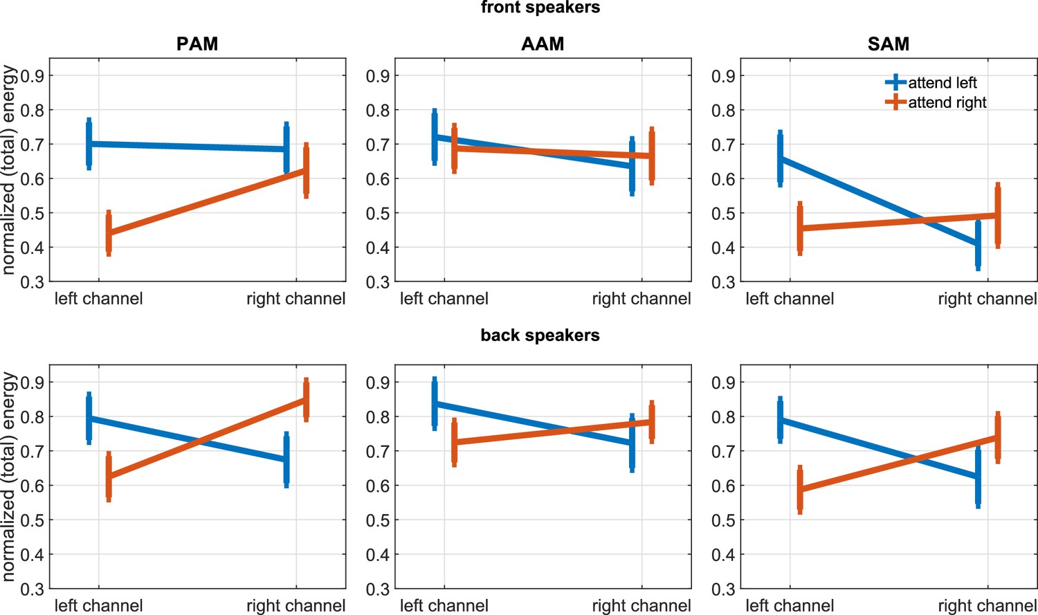
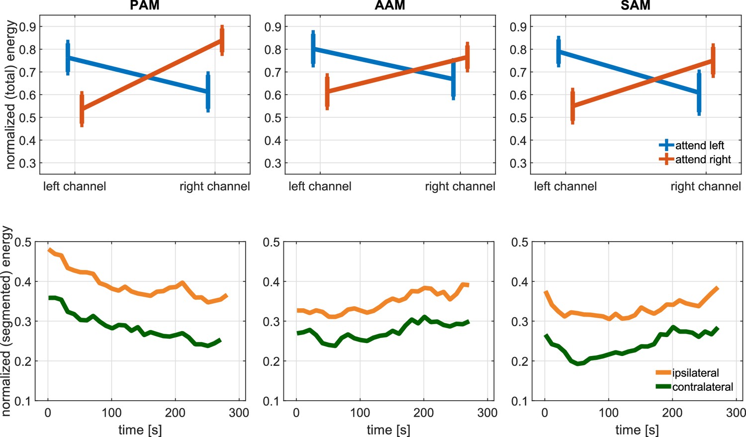
Experiment 2.
Grand average of the PAM, AAM, and SAM activity when stories were played from the front (top) and back speakers (bottom). Shown is the normalized (total) energy of the left/right recording channels during attention to the left or right story (bars represent the standard error). The following figure supplements are available for Figure 5—figure supplement 1. Subband analysis of the described ipsi- vs. contralateral effect for PAM, AAM, and SAM; Figure 5—figure supplement 2. Reported results for a selected narrow frequency band.
Figure 5—figure supplement 1
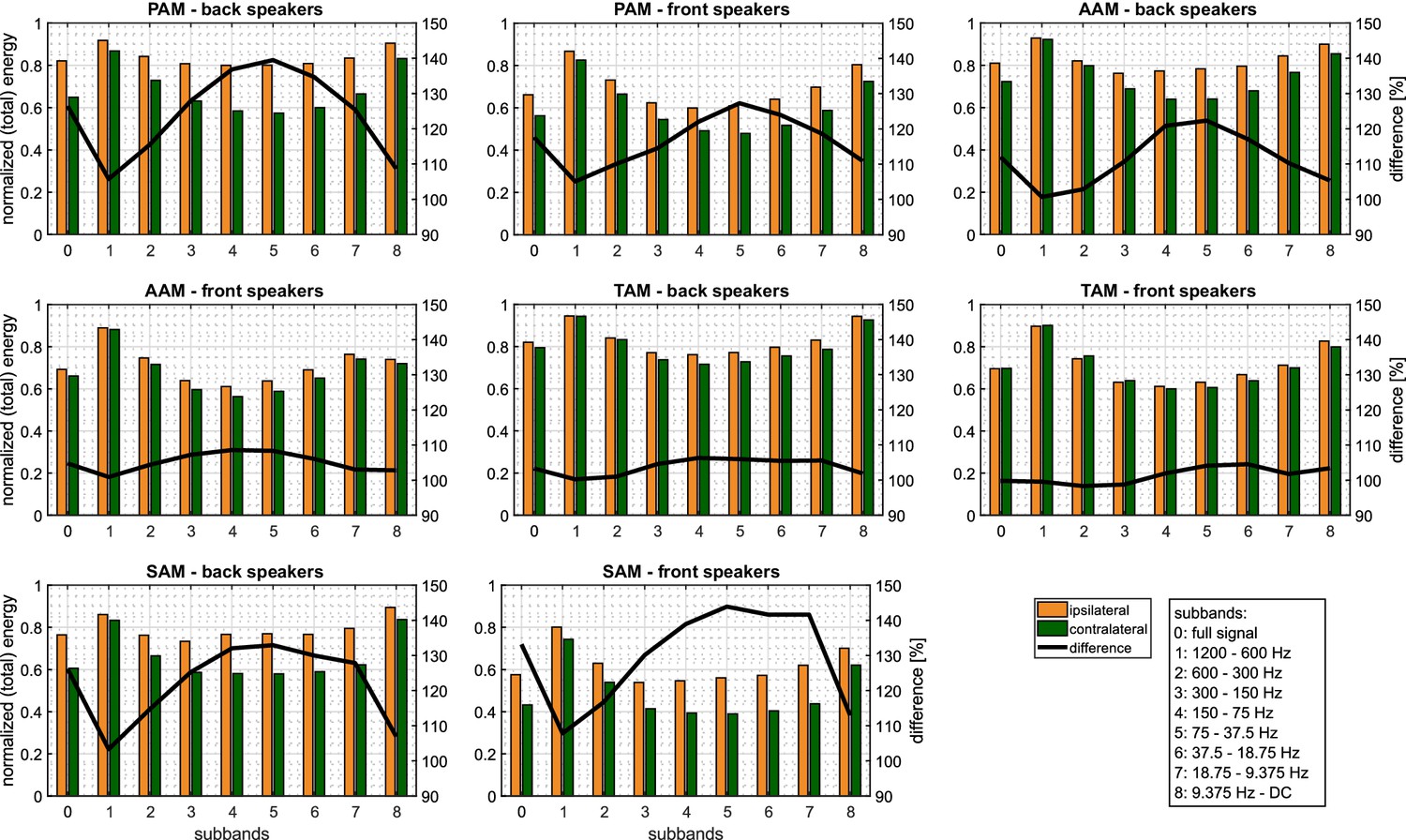
Grand average of the PAM, AAM, and SAM activity when stories were played from front (± 30°) and back speakers (± 120°).
The normalized total energy in each octave-frequency subband is plotted for the left/right recording channels (in the conventional dyadic order) during attention to the left or right story, along with their difference (black line). It is notable that the lowest and highest frequency bands contribute little to the difference. In fact, the middle bands 5 and 6 show the largest attention effect (see also Figure 5—figure supplement 2). Technical decoding applications might make use of this observation.
Figure 5—figure supplement 2
Analogous to Figure 5 and Figure 6, respectively, in the main text but for frequency band 5 (37.5 – 75 Hz): Grand average of the PAM, AAM, and SAM activity when stories were played from the back speakers (± 120°).
Top: normalized total energy of the left/right recording channels when attending to the left or right story (bars represent the standard error). A significant interaction of recording channel and attention direction was observed [PAM, AAM, TAM, SAM: F(1, 19) = 17.2, 8.2, 0.5, and 24.0, respectively; 0.001, 0.01, 0.51, and 0.001; = 0.48, 0.30, 0.02, and 0.56]; Bottom: time–resolved activity after pooling the ipsi– and contralateral signals with a segment–wise normalization. Each sampling point represents the energy induced in consecutive 10 s segments.
Figure 6
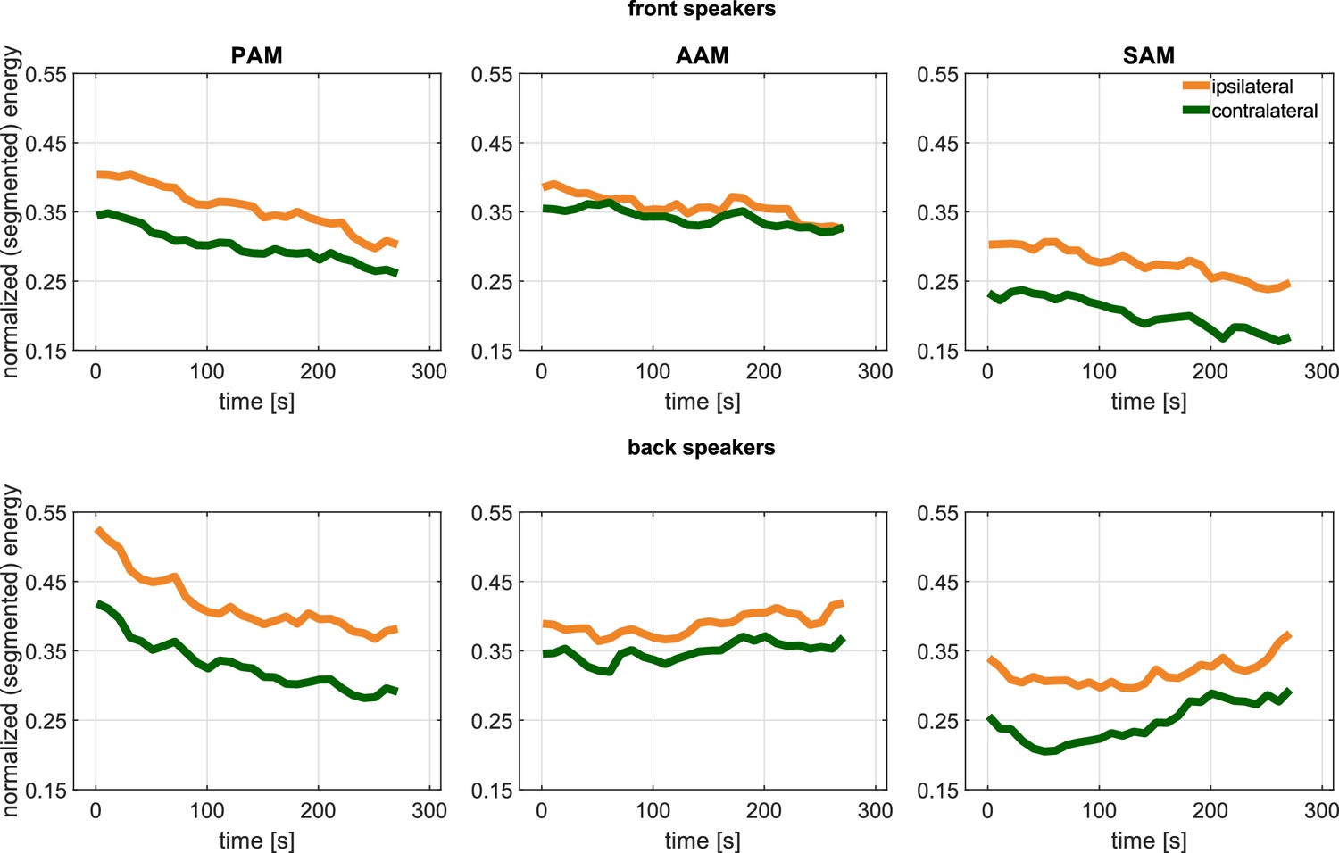
Experiment 2.
Time–resolved activity (each sampling point represents the energy induced in consecutive 10 s segments) after pooling the ipsi– and contralateral signals with a segment–wise normalization for the front (top) and back speakers (bottom).
Figure 7 with 9 supplements
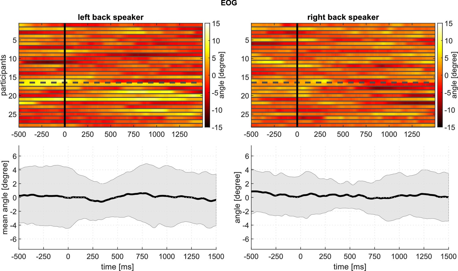
Experiment 1: Averaged horizontal EOG activity at around the time of stimulation from the back speakers, showing an apparent absence of systematic shifts in gaze direction: Top panels: Every row corresponds to the averaged response of one participant.
Gaze angle is encoded in color, such that positive values (yellow) indicate rightward eye movements/positive angles. The top rows (1-16) represent younger adult participants; the bottom rows (17-28), older adults. Bottom panels: Mean and standard deviation based on the above plots.The following figure supplements are available for Figure 7—figure supplement 1. Macrosaccades during reading for one subject as example; Figure 7—figure supplement 2. Boxplots of the EOG for all subjects; Figure 7—figure supplement 3. Density of all detected macrosaccades during Experiment 1; Figure 7—figure supplement 4. Responses of the M. sternocleidomastoideus to stimuli from the front speakers; Figure 7—figure supplement 5. Responses of the M. sternocleidomastoideus to stimuli from the back speakers; Figure 7—figure supplement 6. Responses of the M. frontalis to stimuli from the front speakers; Figure 7—figure supplement 7. Responses of the M. frontalis to stimuli from the back speakers; Figure 7—figure supplement 8. Responses of the M. zygomaticus to stimuli from the front speakers; Figure 7—figure supplement 9. Responses of the M. zygomaticus to stimuli from the back speakers.
Figure 7—figure supplement 1
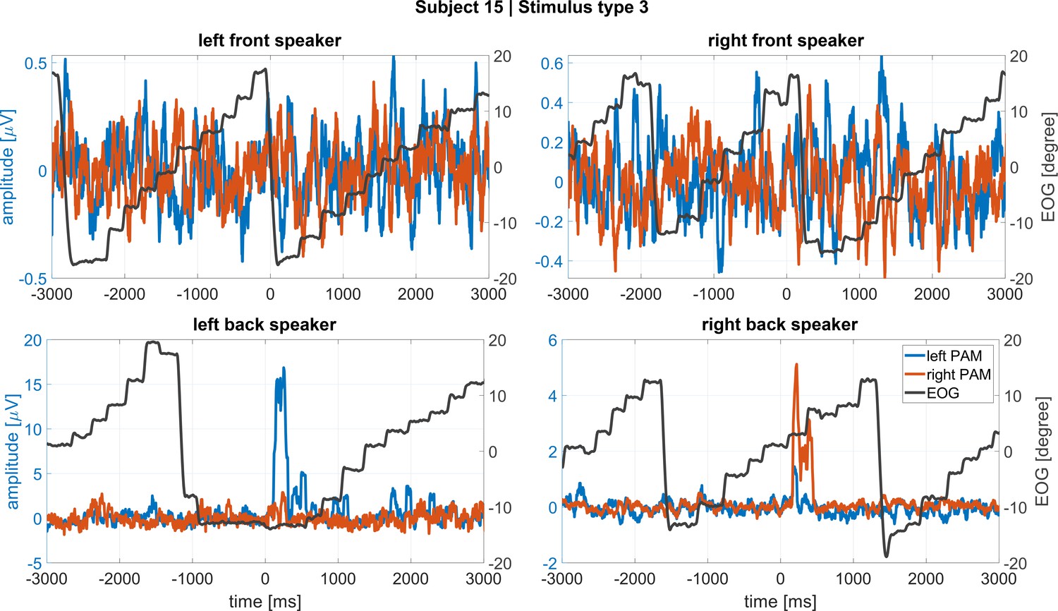
Macrosaccades during reading in Experiment one as recorded by means of horizontal EOG (black line) along with time-synchronized EMG from left and right PAM (blue and orange lines, respectively).
This participant (# 15) had large, clear PAM responses. Different trials are shown in the four panels. Note that muscle activations occur without saccades and large saccades occur without muscle responses.
Figure 7—figure supplement 2
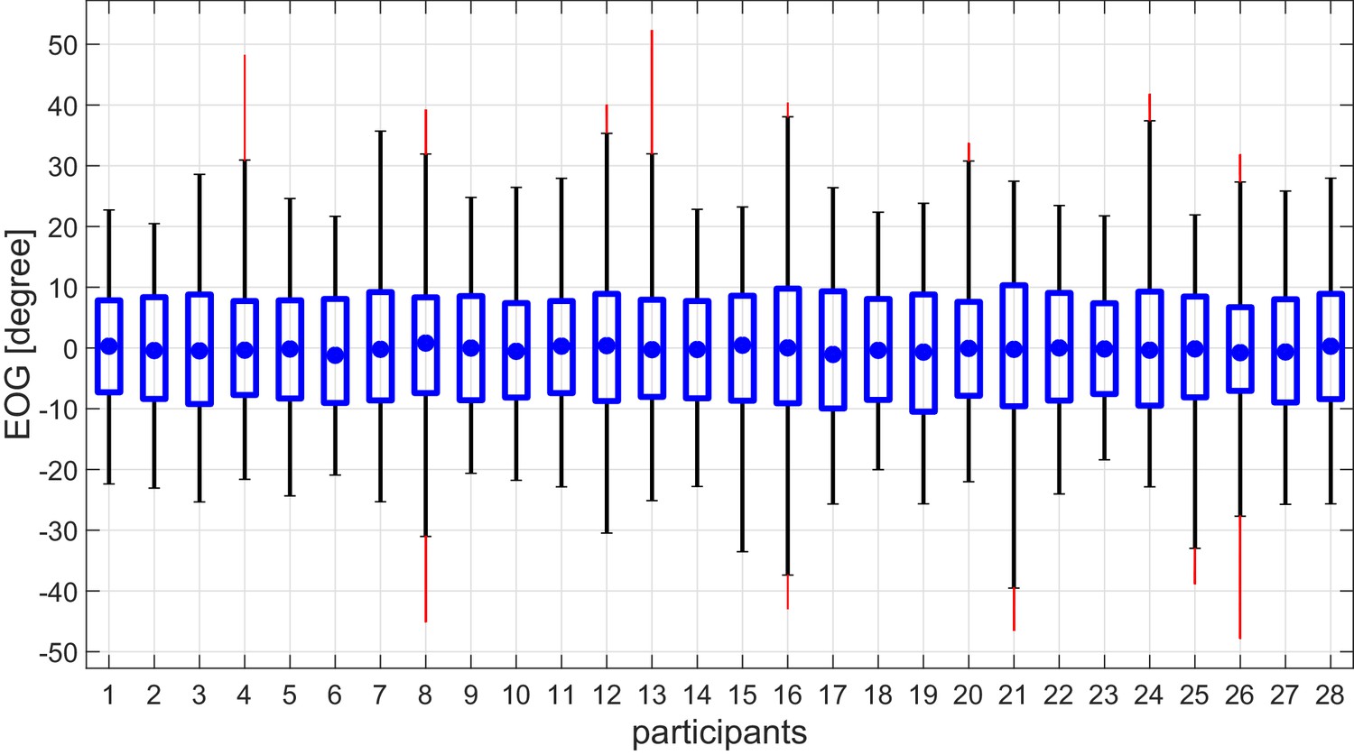
Boxplots of EOG signals from all subjects in Experiment 1.
Every stimulus presentation, including 3 s long pre– and poststimulus intervals, were included. Blue dots mark the median, outliers (data points beyond 1.5 x interquartile range) are displayed in red. Gaze shifts between the edges of the text that subjects were reading from during this experiment generated the largest EOG values. These shifts can be estimated in the upper and lower whiskers.
Figure 7—figure supplement 3
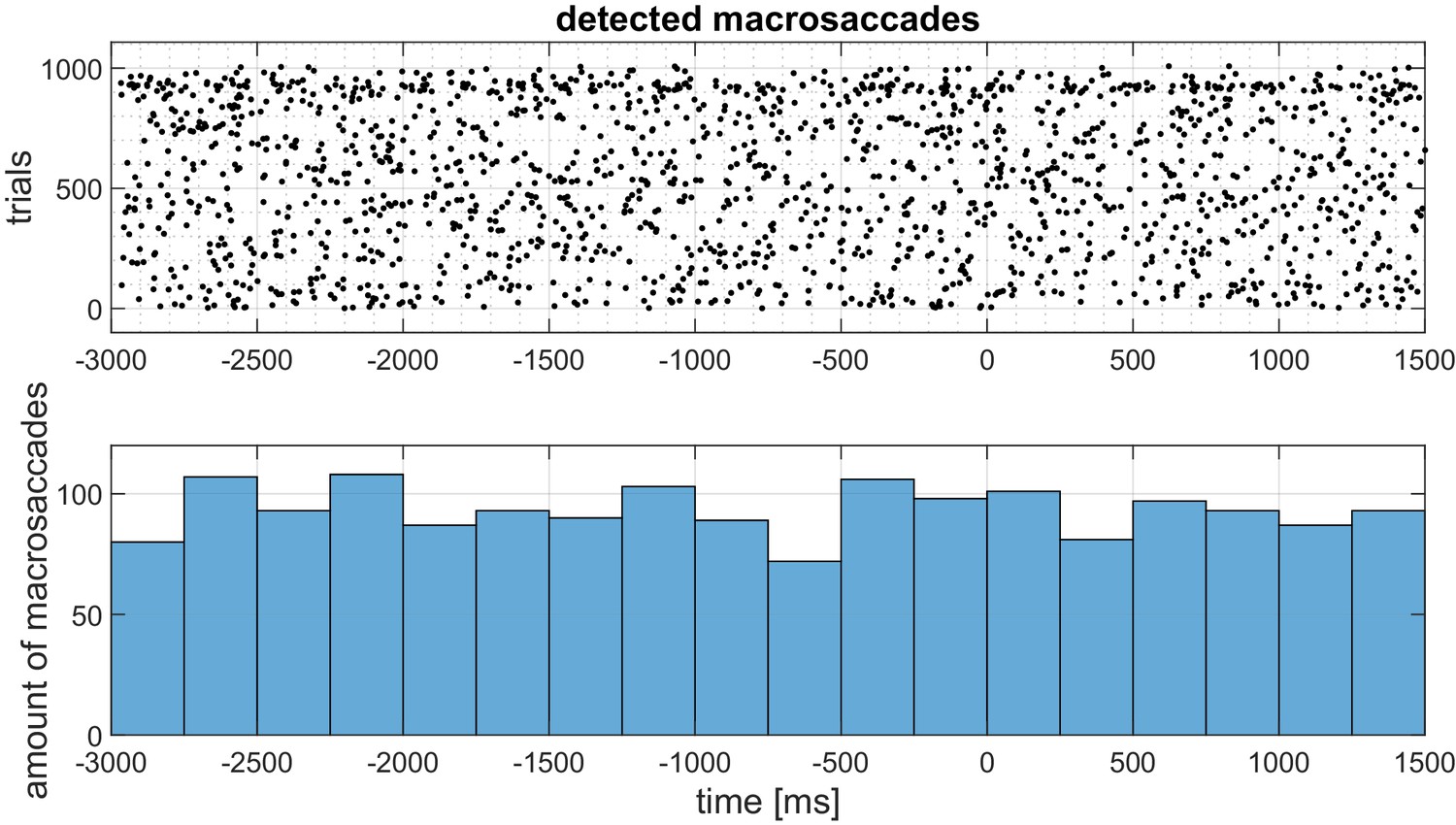
Density of detected macrosaccades during Experiment 1.
Top plot: Every line corresponds to one stimulus presentation (trials). Detected macrosaccades are marked by black dots. Across all subjects, 1008 stimuli were presented. Bottom plot: Histogram of detected macrosaccades with respect to time. Macrosaccades were detected by calculating the forward differences with samples (62.5 ms) for every point and thresholding . Both and were determined empirically to reliably detect saccades when the subjects jump from a given line to the next one.
Figure 7—figure supplement 4
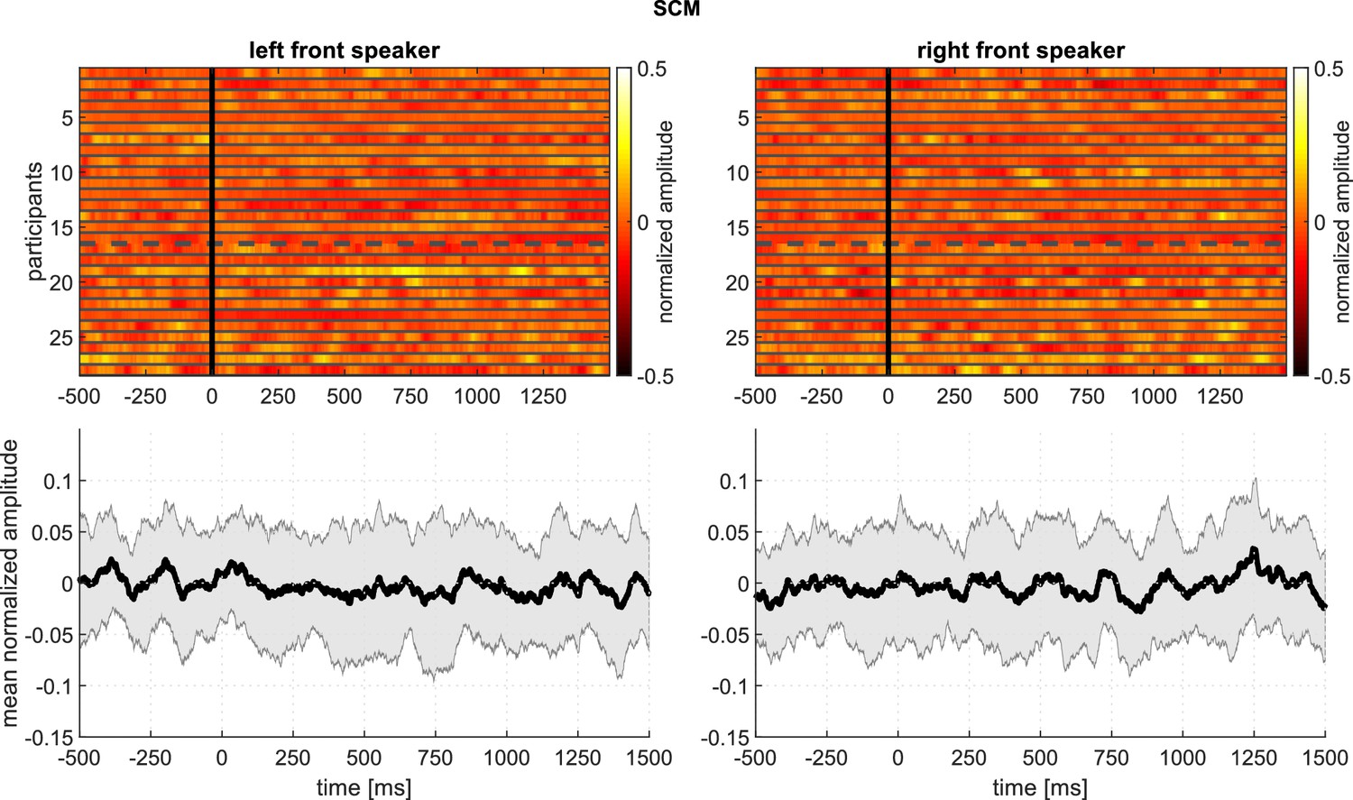
Experiment 1 – Responses of the M. sternocleidomastoideus (M.SCM) to stimuli from the front speakers, showing intersubject variability: Top panels: Every row corresponds to the averaged response of one participant.
Amplitude is encoded in color. The top rows (1-16) represent younger adult participants; the bottom rows (17-28), older adults. Bottom panels: Mean and standard deviation based on the above plots.
Figure 7—figure supplement 5
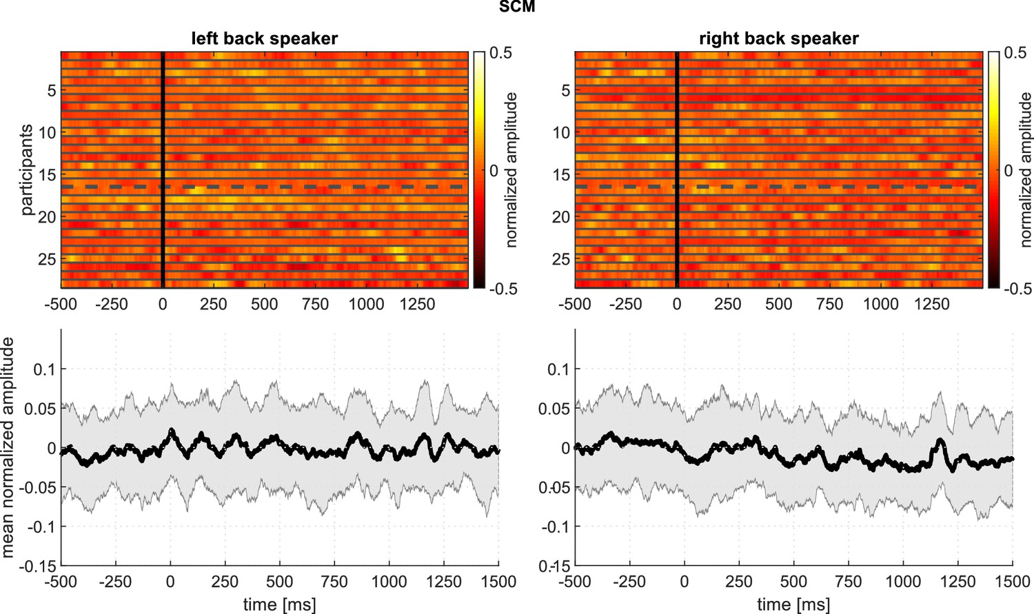
Experiment 1 – Responses of the M. sternocleidomastoideus (M.SCM) to stimuli from the back speakers, showing intersubject variability: Top panels: Every row corresponds to the averaged response of one participant.
Amplitude is encoded in color. The top rows (1-16) represent younger adult participants; the bottom rows (17-28), older adults. Bottom panels: Mean and standard deviation based on the above plots.
Figure 7—figure supplement 6
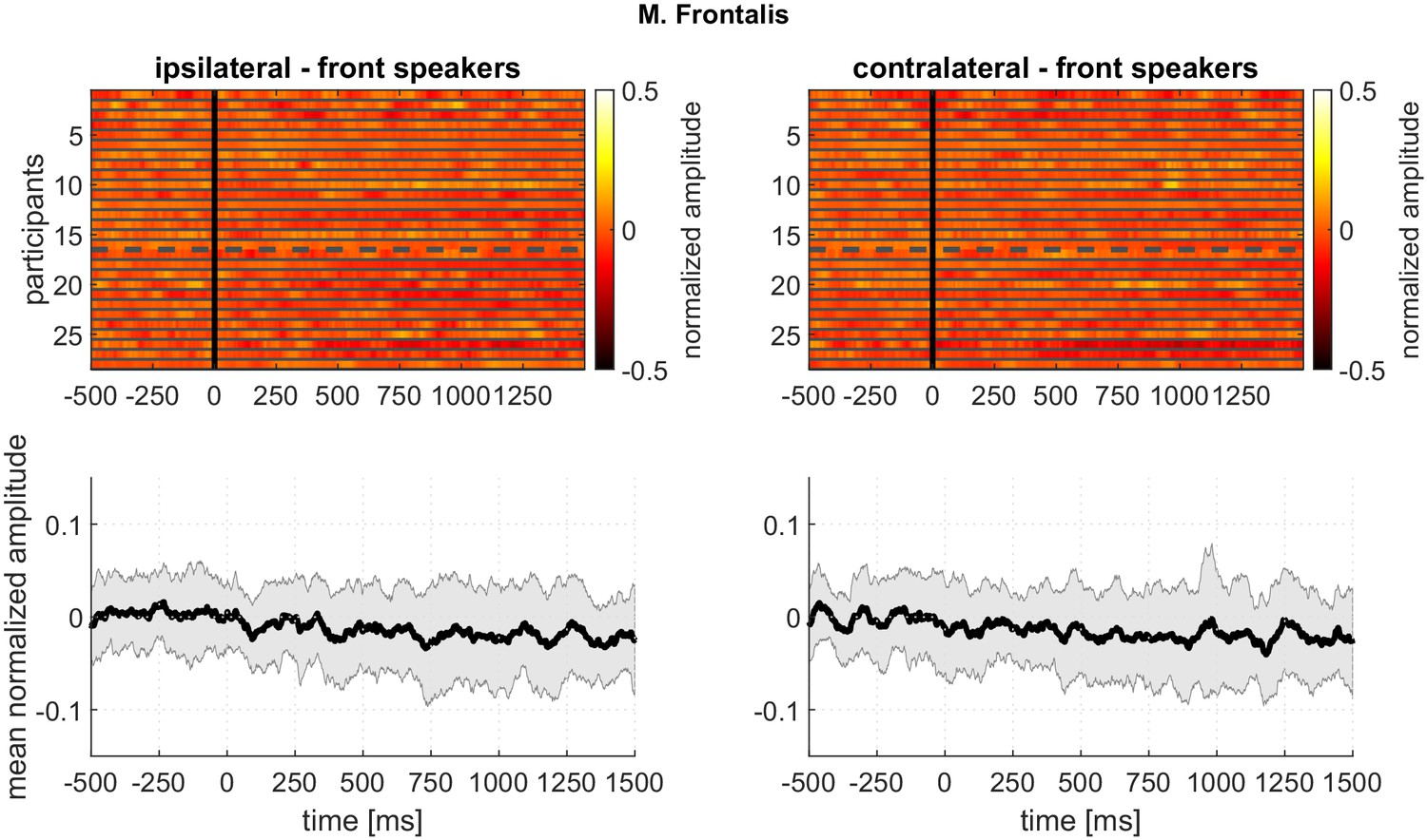
Experiment 1 – Responses of the frontalis muscle to stimuli from the front speakers, showing intersubject variability: Top panels: Every row corresponds to the averaged response of one participant.
Amplitude is encoded in color. The top rows (1-16) represent younger adult participants; the bottom rows (17-28), older adults. Bottom panels: Mean and standard deviation based on the above plots.
Figure 7—figure supplement 7
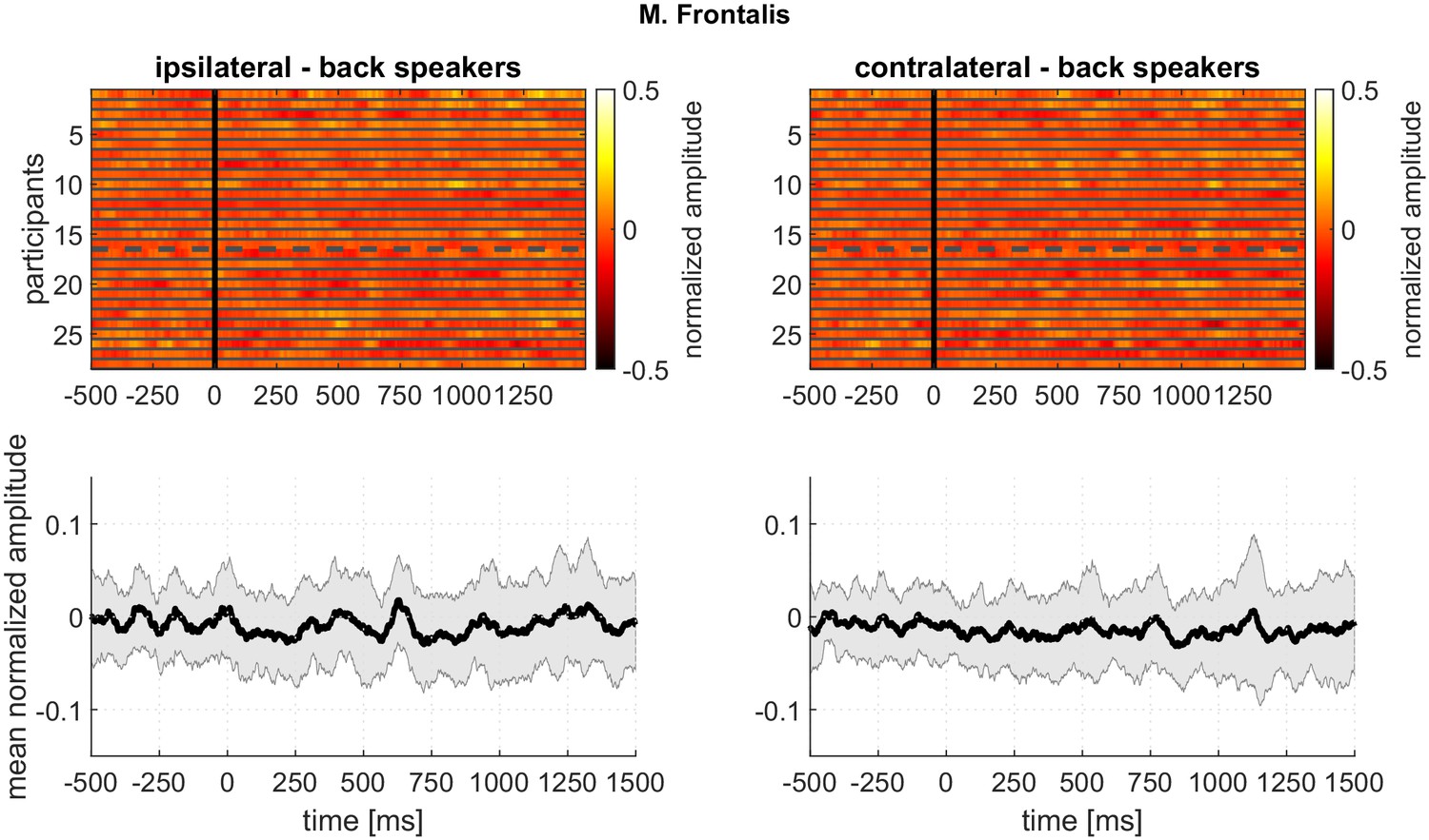
Experiment 1 – Responses of the frontalis muscle to stimuli from the back speakers, showing intersubject variability: Top panels: Every row corresponds to the averaged response of one participant.
Amplitude is encoded in color. The top rows (1-16) represent younger adult participants; the bottom rows (17-28), older adults. Bottom panels: Mean and standard deviation based on the above plots.
Figure 7—figure supplement 8
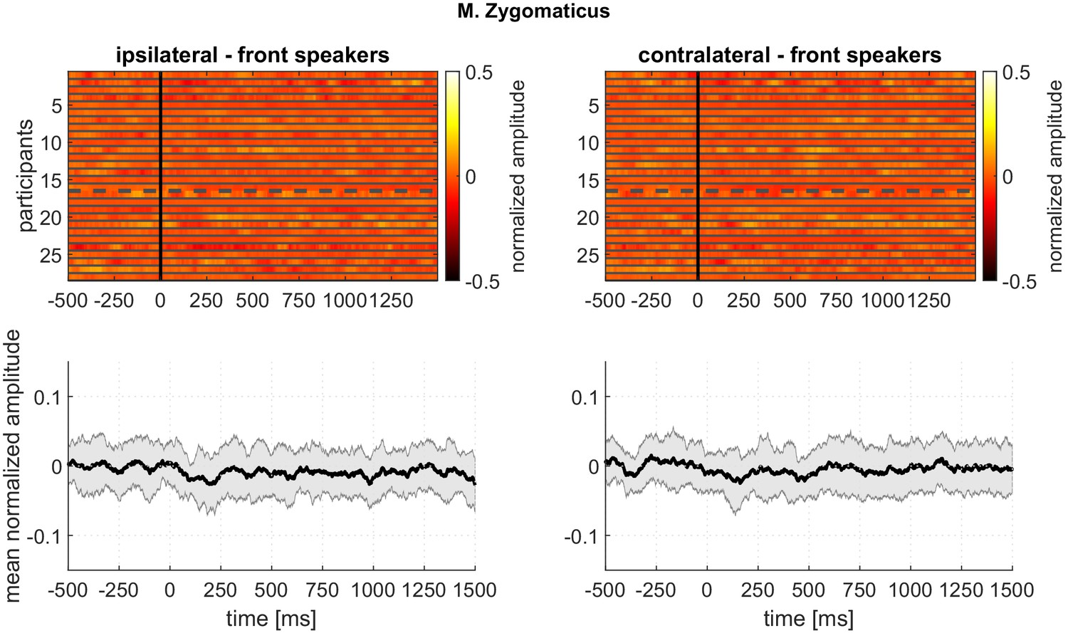
Experiment 1 – Responses of the zygomaticus muscle to stimuli from the front speakers, showing intersubject variability: Top panels: Every row corresponds to the averaged response of one participant.
Amplitude is encoded in color. The top rows (1-16) represent younger adult participants; the bottom rows (17-28), older adults. Bottom panels: Mean and standard deviation based on the above plots.
Figure 7—figure supplement 9
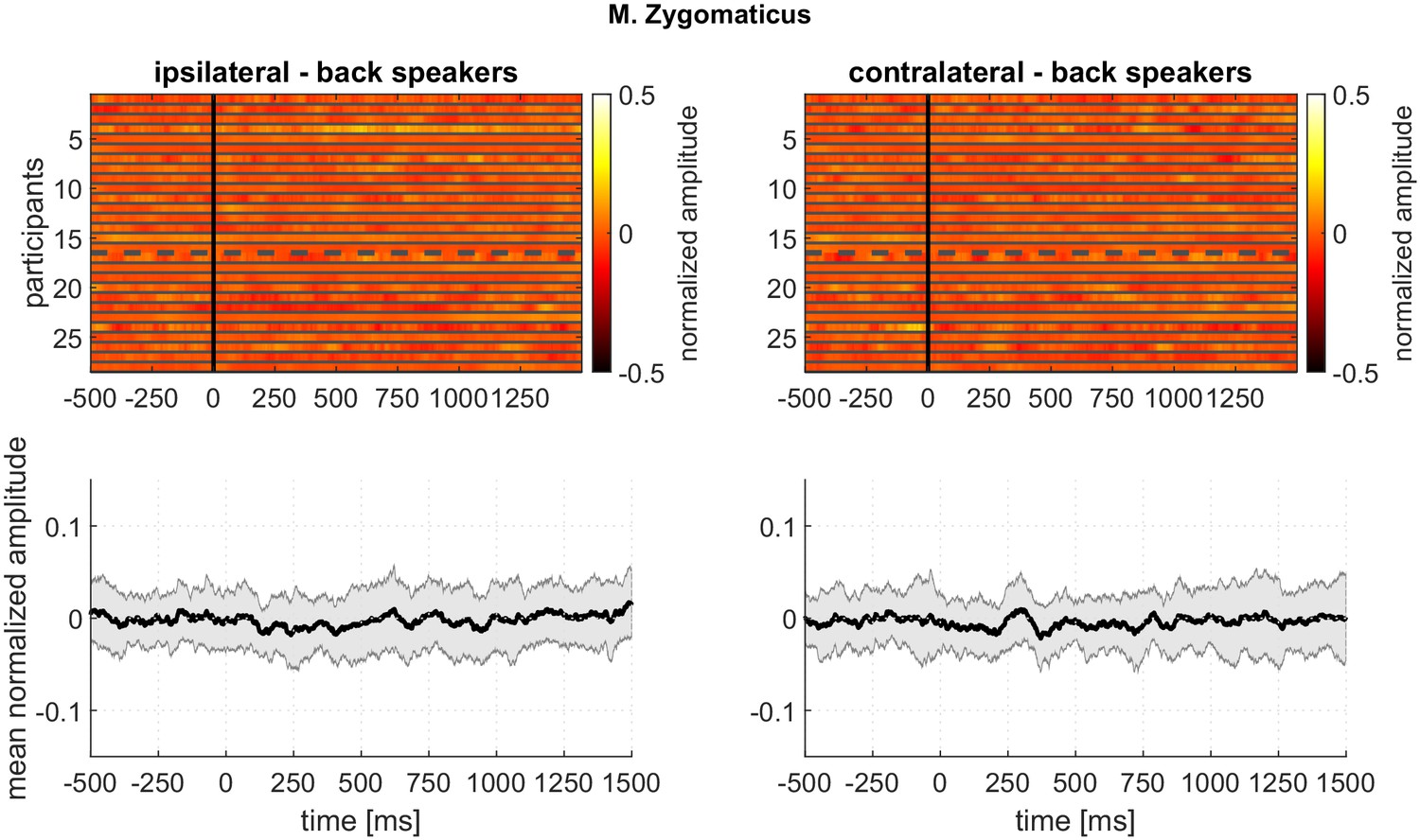
Experiment 1 – Responses of the zygomaticus muscle to stimuli from the back speakers, showing intersubject variability: Top panels: Every row corresponds to the averaged response of one participant.
Amplitude is encoded in color. The top rows (1-16) represent younger adult participants; the bottom rows (17-28), older adults. Bottom panels: Mean and standard deviation based on the above plots.
Figure 8 with 2 supplements
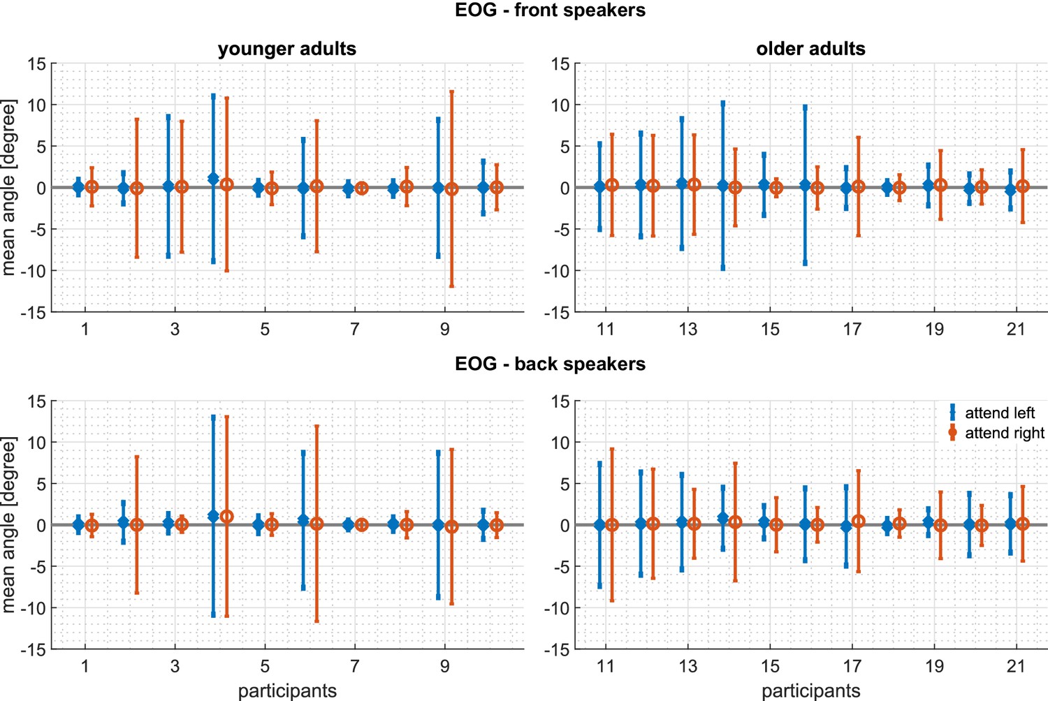
Experiment 2: Intrasubject variability of the horizontal EOG: Mean and standard deviations of the EOG during the complete trial of every participant.
Top panels: attending the front speakers. Bottom panels: attending the back speakers. Left panels: younger adults. Right panels: older adults. Blue represents the EOG when attending the left, red when attending the right speaker. A positive EOG indicates that the gaze is directed toward the side of the attended speaker. Note that the deviation of the mean from is well within one standard deviation and therefore indicates that participants did not systematically divert their gaze to the attended speaker. The following figure supplements are available for Figure 8—figure supplement 1. Time-resolved EOG analysis in Experiment 2; Figure 8—figure supplement 2. Activity of the frontalis and zygomaticus muscle in Experiment 2.
Figure 8—figure supplement 1
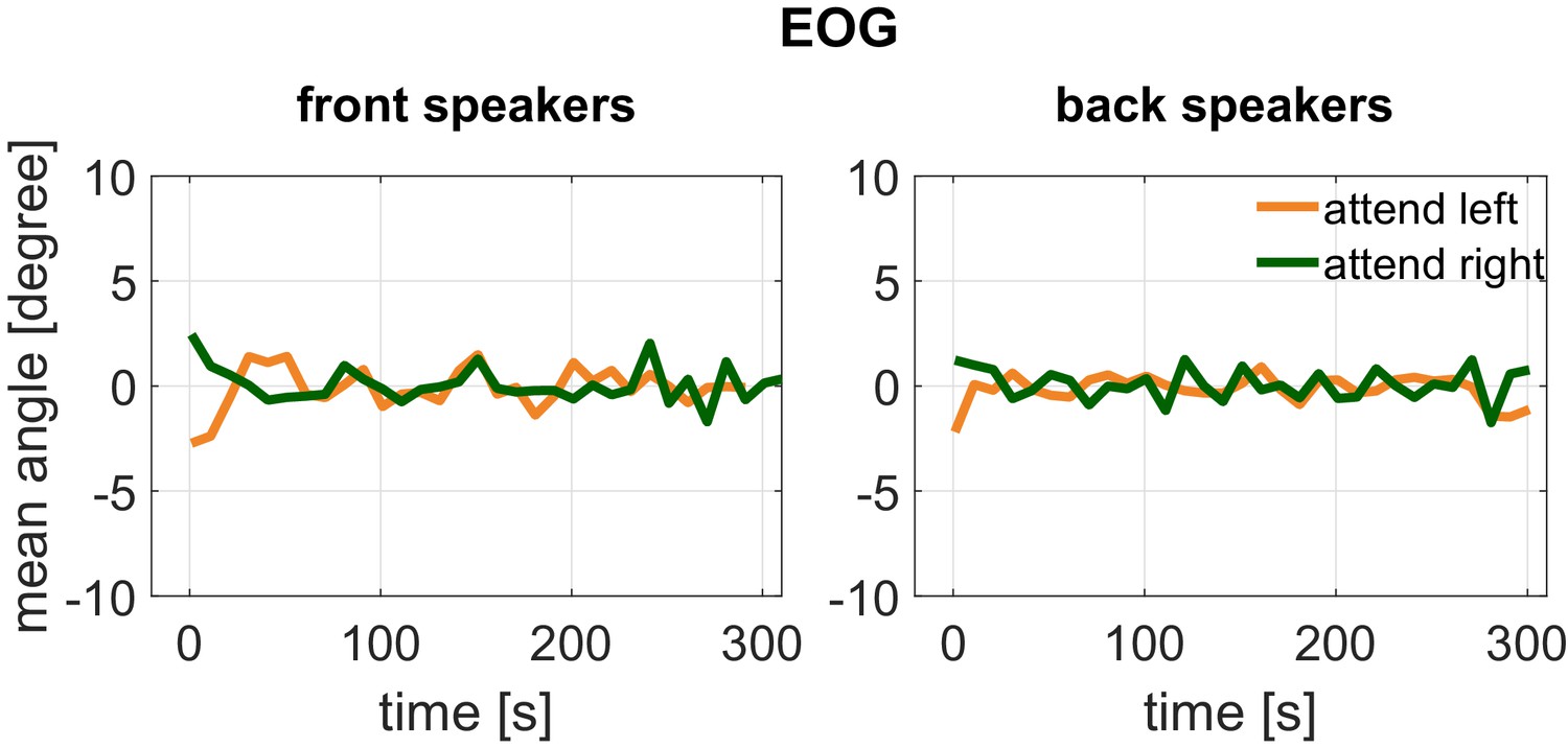
Time-resolved activity (sampling points represent the energy within consecutive 10 s segments) after pooling the ipsi- and contralateral EOG signals for the front (left) and back speakers (right) in Experiment 2.
Figure 8—figure supplement 2
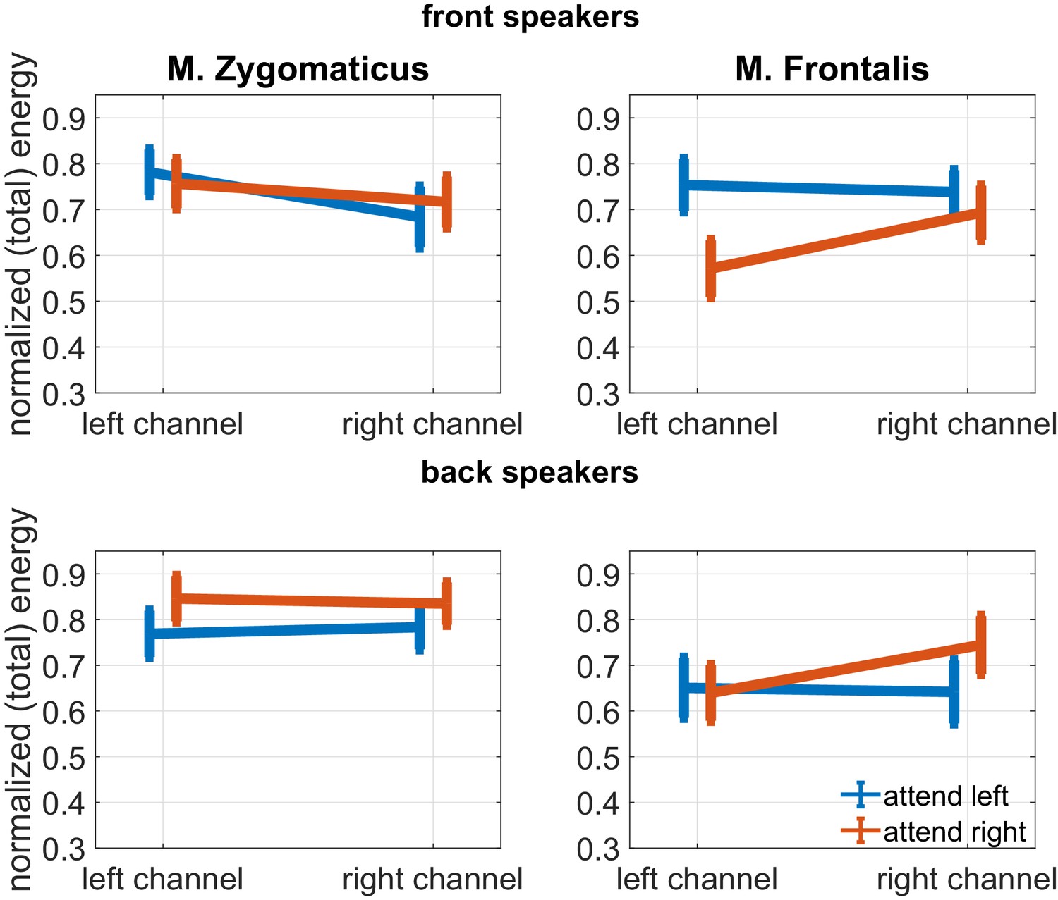
Grand average of the zygomaticus and frontalis muscle activity when stories were played from the front (top row) and back speakers (bottom row) in Experiment 2.
Shown is the normalized (total) energy of the left/right recording channels during attention to the left or right story (bars represent the standard error). There was no significant interaction of recording channel and attention direction [zygomaticus, frontalis: F(1, 19) = 0.13 and 3.44; 0.73 and 0.08; = 0.007 and 0.15].
Author response image 1
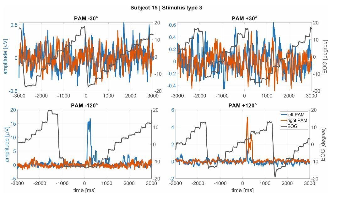
Macrosaccades in the EOG (black line) during reading in Experiment 1 for subject 15 as example (a subject with large, clear PAM activations).
It is noticeable that the muscle activations are not linked to the macrosaccades.
Author response image 2
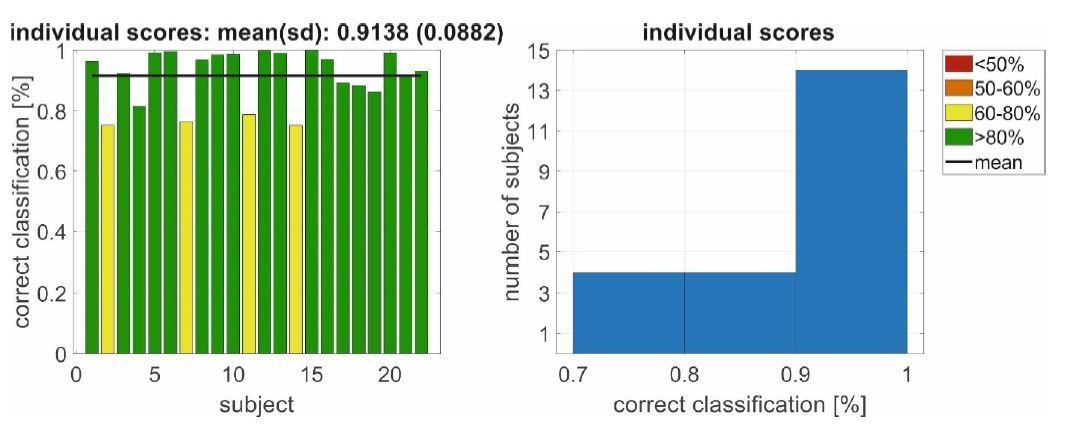
Left/right decoding performance for a conjoint classification of PAM/SAM EMG using an individualized decoding scheme in Experiment 2.
Author response image 3
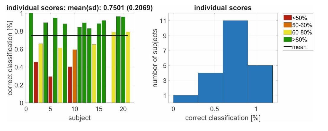
Left/right decoding performance for a conjoint classification of PAM/SAM EMG using an(non-individualized) decoding scheme in Experiment 2 with a leave-one-participant-out cross validation.
Author response image 4
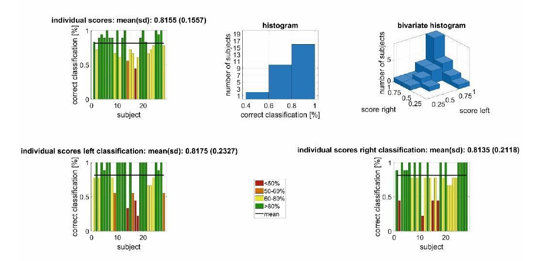
Left/right decoding performance for a conjoint classification of PAM/AAM/SAM/TAM EMG using an (non-individualized) decoding scheme in Experiment 1 with a leave-one-participant-out cross validation.
Videos
Video 1
Experiment 1 –Ear movement example from a trial with a novel sound at the right posterior speaker in Experiment 1.
The right half of the display portrays evoked movements of the ipsilateral pinna in three ways. The large video clip of the pinna uses digital magnification to render the overall pattern of movement apparent. The color overlay in these videos indicates the motion magnitude. Just below the video and to the right, an unrectified EMG recording of the postauricular muscle is shown in co-registration with the video. The global head motion was reduced by a 2-dimensional rigid pre-registration with respect to a set of manually specified reference points on the head (see also Figure 2—figure supplement 1). The 3-dimensional graph medial to the 2-D graph includes a vector that indicates moment-by-moment changes in EMG activity of the superior auricular muscle (SAM, the vertical axis), transverse auricular muscle (TAM, a horizontal axis), and the difference between activity in the posterior and anterior auricular muscles (PAM-AAM, the other horizontal axis). The left half of this video gives corresponding information for the contralateral ear which, consistent with evidence presented in the main text, was not as active as the ipsilateral one.
Video 2
Experiment 1 –The right ear example from the previous video, but with four different videos in sequence.
The first video of the sequence shows the raw recording (without digital magnification). The second video shows the digitally magnified motion, the third video shows the magnified motion with color overlay as in the previous video supplement, and the fourth video shows the three dimensional motion from a different angle. This video sequence shows the impact of the digital motion magnification and the depth information about ear motion that can be derived from a stereo computer vision setup such as the one used here.
Video 3
Experiment 2 –Ear movement example from a participant who exhibited exceptionally large, long-lasting involuntary auricular muscle activations and ear motion during the endogenous attention task in Experiment 2.
The attention of the participant was directed to the story played from the posterior right speaker. The organization of the plots and co-registration is as in Video 1. However, this time the raw videos without digital magnification are shown. The raw videos are played faster, time-locked to the time axis given in minutes in the one dimensional plots of the rectified postauricular muscle activity. Note that time-axis reflects the entire timeline including the instructions and the introduction to the stories before the directional listening task. The listening task started at approximately 2 min. The video also documents the end of the listening task (around 7 min) accompanied with a time–locked offset of the muscle activation and pinna displacement. A causal relation of the rectified postauricular muscle activity and the motion magnitude in the videos is clearly noticeable, especially for the ipsilateral ear.
Additional files
-
Supplementary file 1
Table Supplements for Experiment 2.
- https://cdn.elifesciences.org/articles/54536/elife-54536-supp1-v1.pdf
-
Transparent reporting form
- https://cdn.elifesciences.org/articles/54536/elife-54536-transrepform-v1.pdf
Download links
A two-part list of links to download the article, or parts of the article, in various formats.
Downloads (link to download the article as PDF)
Open citations (links to open the citations from this article in various online reference manager services)
Cite this article (links to download the citations from this article in formats compatible with various reference manager tools)
Vestigial auriculomotor activity indicates the direction of auditory attention in humans
eLife 9:e54536.
https://doi.org/10.7554/eLife.54536


