Figures and data in Efficient sampling and noisy decisions

Figures
Tables
Additional files

7 figures, 1 table and 1 additional file

Figures

Figure 1

Download asset Open asset

Architecture of the sampling mechanism.

Each processing unit receives noisy versions of the input $v$ , where the noisy signals are i.i.d. additive random signals independent of $v$ . The output of the neuron for each sample is 'high' (one) reading if $v - η > τ$ and zero otherwise. The noisy percept of the input is simply the sum of the outputs of each sample given by $k$ .

Figure 2

Download asset Open asset

Overview of our theory and differences in encoding rules.

(a) Schematic representation of our theory. Left: example prior distribution $f (v)$ of values $v$ encountered in the environment. Right: Prior distribution in the encoder space (Equation 2) due to optimal encoding (Equation 3). This optimal mapping determines the probability $θ$ of generating a 'high' or 'low' reading. The ex-ante distribution over $θ$ that guarantees maximization of mutual information is given by the arcsine distribution (Equation 2). (b) Encoding rules $θ (v)$ for different decision strategies under binary sampling coding: accuracy maximization (blue), reward maximization (red), DbS (green dashed). (c) Mutual information $I (v, k)$ for the different encoding rules as a function of the number of samples $n$ . As expected $I (v, k)$ increases with $n$ , however the rule that results in the highest loss of information is DbS. (d) Discriminability thresholds $d$ (log-scaled for better visualization) for the different encoding rules as a function of the input values $v$ for the prior $f (v)$ given in panel a. (e) Graphical representation of the perceptual accuracy optimization landscape. We plot the average probability of correct responses for the large- $n$ limit using as benchmark a Beta distribution with parameters $a$ and $b$ . The blue star shows the average error probability assuming that $f (θ)$ is the arcsine distribution (Equation 2), which is the optimal solution when the prior distribution $f$ in known. The blue open circle shows the average error probability based on the encoding rule assumed in DbS, which is located near the optimal solution. Please note that when formally solving this optimization problem, we did not assume a priori that the solution is related to the beta distribution. We use the beta distribution in this figure just as a benchmark for visualization. Detailed comparison of performance for finite $n$ samples is presented in Appendix 7.

Figure 3 with 3 supplements

Download asset Open asset

Experimental design, model simulations and recovery.

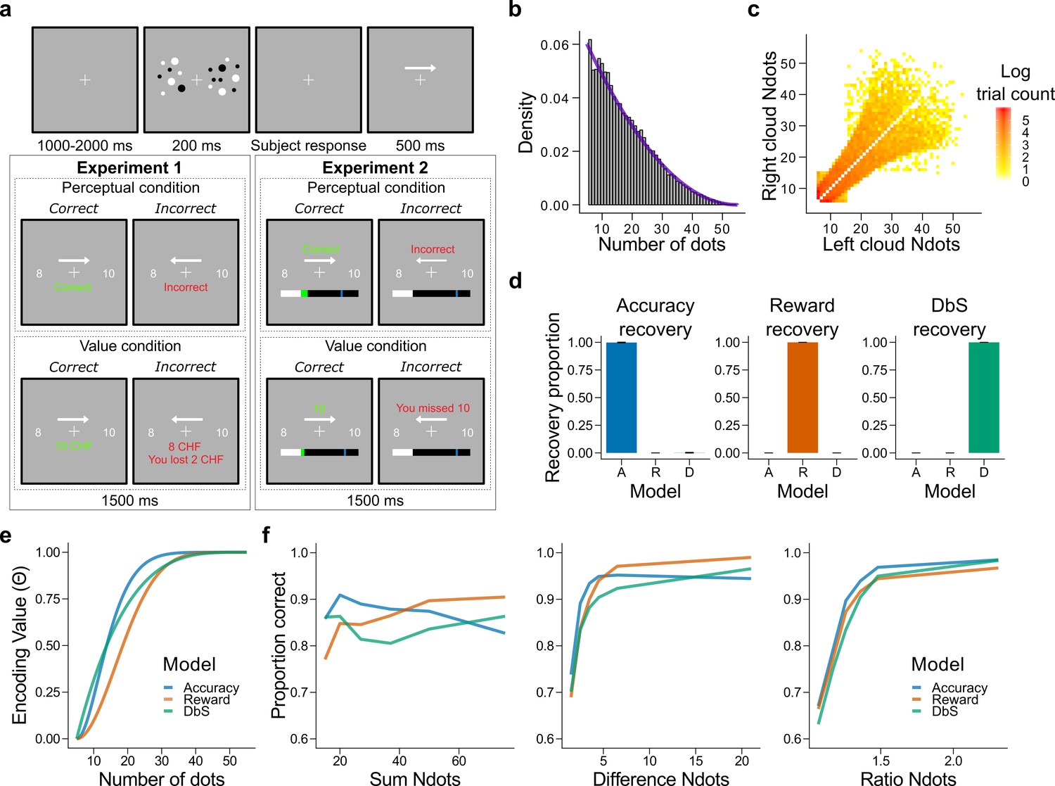
(a) Schematic task design of Experiments 1 and 2. After a fixation period (1–2 s) participants were presented two clouds of dots (200 ms) and had to indicate which cloud contained the most dots. Participants were rewarded for being accurate (perceptual condition) or for the number of dots they selected (value condition) and were given feedback. In Experiment 2 participants collected on correctly answered trials a number of points equal to a fixed amount (perceptual condition) or a number equal to the dots in the cloud they selected (value condition) and had to reach a threshold of points on each run. (b) Empirical (grey bars) and theoretical (purple line) distribution of the number of dots in the clouds of dots presented across Experiments 1 and 2. (c) Distribution of the numerosity pairs selected per trial. (d) Synthetic data preserving the trial set statistics and number of trials per participant used in Experiment 1 was generated for each encoding rule (Accuracy (left), Reward (middle), and DbS (right)) and then the latent-mixture model was fitted to each generated dataset. The figures show that it is theoretically possible to recover each generated encoding rule. (e) Encoding function $θ (v)$ for the different sampling strategies as a function of the input values $v$ (i.e., the number of dots). (f) Qualitative predictions of the three models (blue: Accuracy, red: Reward, green: Decision by Sampling) on trials from Experiment 1 with $n = 25$ . Performance of each model as a function of the sum of the number of dots in both clouds (left), the absolute difference between the number of dots in both clouds (middle) and the ratio of the number of dots in the most numerous cloud over the less numerous cloud (right).

Figure 3—figure supplement 1

Download asset Open asset

Model recovery for $α$ fixed.

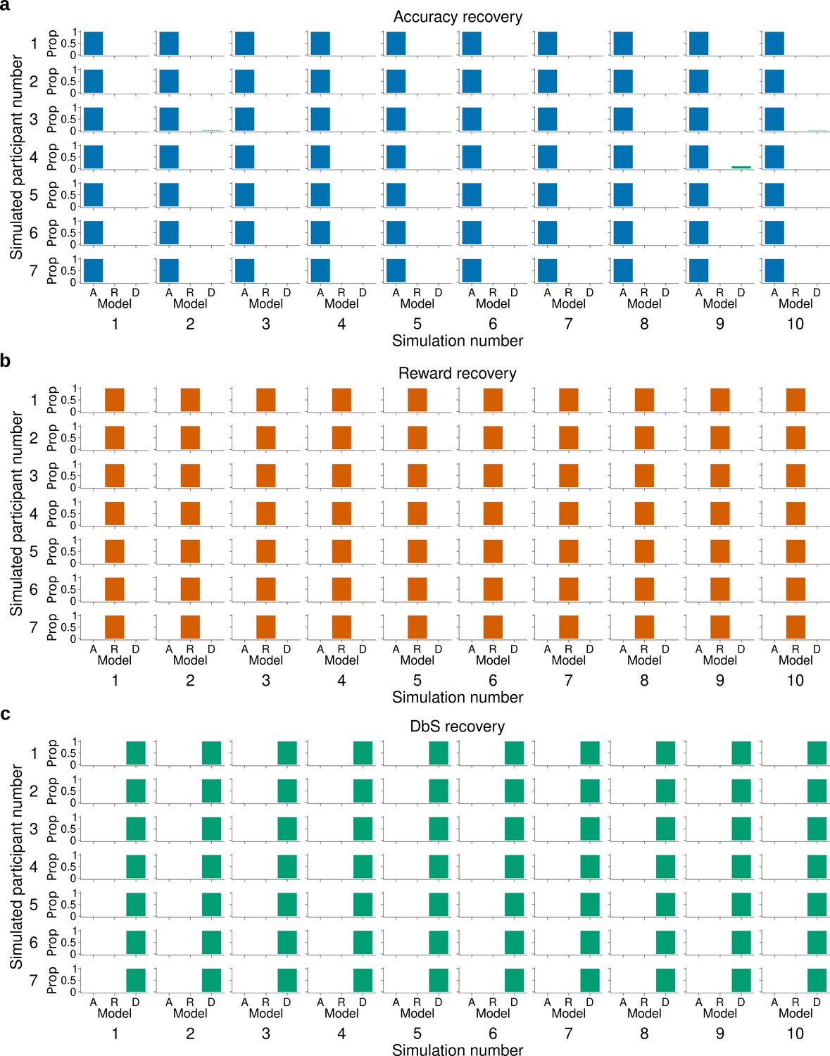
The latent-mixture model was fitted to synthetic data obtained by simulating 10 times each encoding rule on the trials from participants of Experiment 1. This also means that we used the same number of trials per condition that each participant experienced in our experiments. Each histogram shows the proportion (Prop) of the recovered encoding rule for synthetic data from (a) the accuracy maximizing encoding rule $θ_{A}$ , (b) the reward maximizing encoding rule $θ_{R}$ , and (c) decision by sampling $θ_{D}$ . The latent mixture model can accurately recover the underlying encoding rule. In this model the $α$ parameter was set to 2.

Figure 3—figure supplement 2

Download asset Open asset

Model recovery with both $α$ and $n$ as free parameters.

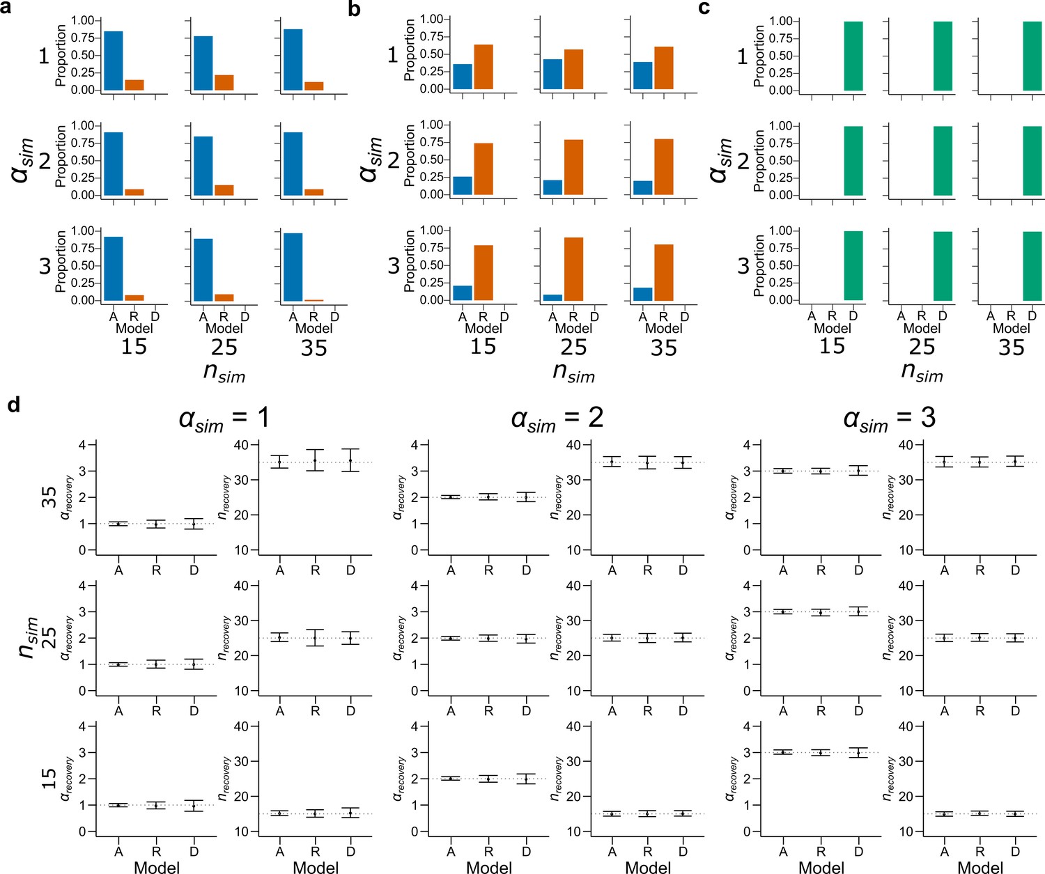
Synthetic data preserving the trial set statistics and number of trials per participant used in Experiment 1 was generated 100 times for each encoding rule with various values of $α$ and $n$ . A model for each encoding rule was fitted to the data using maximum likelihood estimators with $α$ and $n$ as free parameters. The histograms represent the proportion of best fitting models for data generated by (a) Accuracy, (b) Reward and (c) DbS models. Results are shown for different simulated values of $α$ (top: $α_{s i m} = 1$ , middle: $α_{s i m} = 2$ and bottom: $α_{s i m} = 3$ ) and $n$ (left: $n_{s i m} = 15$ , middle: $n_{s i m} = 25$ and right: $n_{s i m} = 35$ ). While DbS is always well recovered, the Accuracy and Reward models tend to be confounded with each other. (d) This same synthetic data were fitted with its generating model with $α$ and $n$ as free parameters using maximum likelihood estimators. Results are shown for different simulated values of $α$ (first and second columns: $α_{s i m} = 1$ , third and fourth columns: $α_{s i m} = 2$ and fifth and sixth columns: $α_{s i m} = 3$ ) and $n$ (top: $n_{s i m} = 35$ , middle: $n_{s i m} = 25$ and bottom: $n_{s i m} = 15$ ). Error bars represent ± SD of the recovered parameter across simulations. The parameters are well recovered by the respective generating model.

Figure 3—figure supplement 3

Download asset Open asset

Discriminability differences between the different encoding rules.

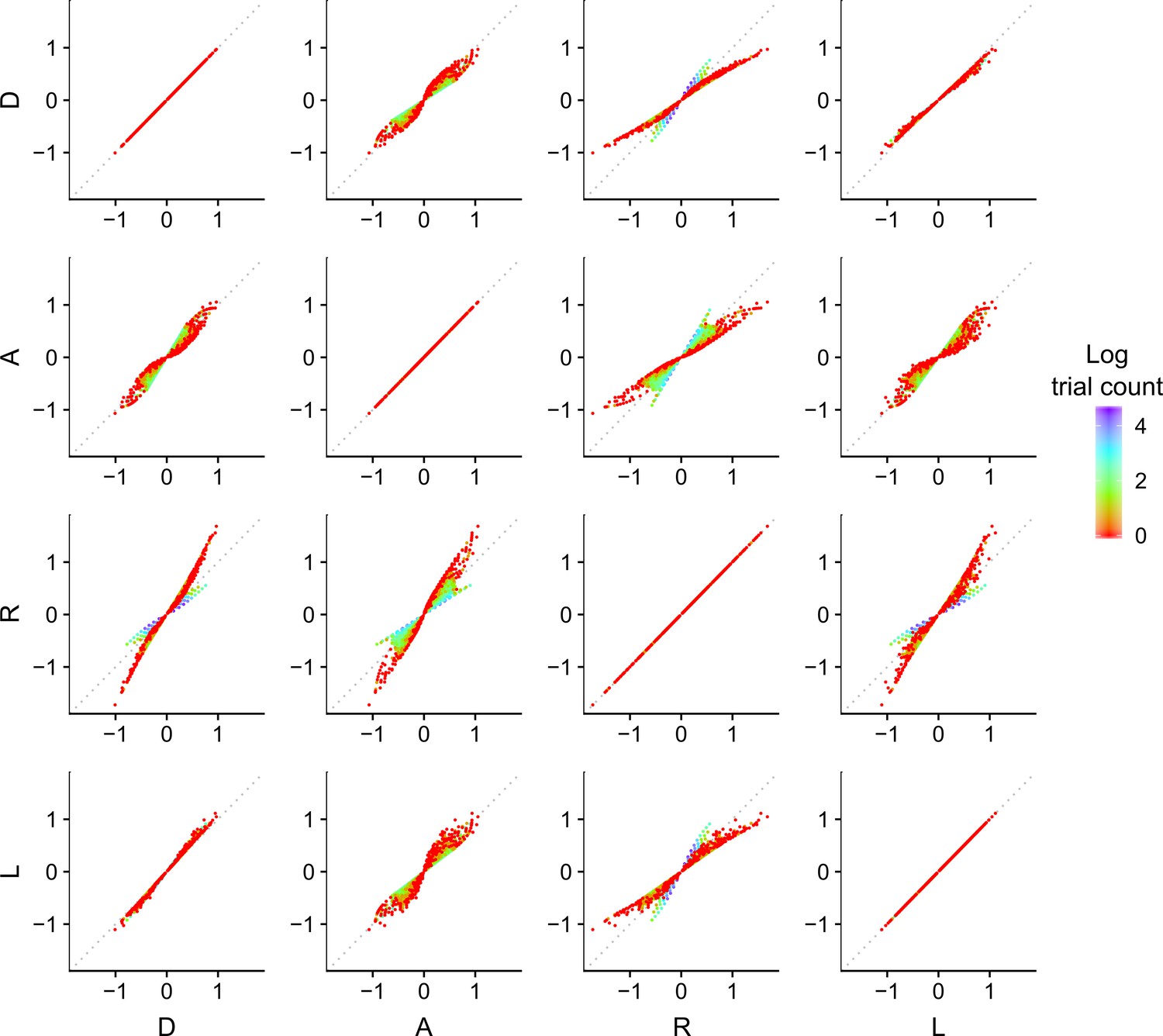
This figure illustrates the discriminability differences between the different encoding rules considered in this study. Each dot represents the discriminability value for a pair of numerosity values $v_{1}$ and $v_{2}$ presented on a given trial to the participants in Experiment 1. For the sampling models, the discriminability rule is defined as
$\frac{θ (v_{1}) - θ (v_{2})}{\sqrt{θ (v_{1}) (1 - θ (v_{1})) + θ (v_{2}) (1 - θ (v_{2}))}},$
where $θ$ corresponds to the respective Accuracy maximizing (A), Reward maximizing (R) or Decision by Sampling (D) encoding rules. For the logarithmic model (L) the discriminability rule is defined as
$log (v_{1}) - log (v_{2}) .$
The color of each dot represents the log of the number of occurrences for the pairs of input values $v_{1}$ and $v_{2}$ . Note that the encoding values of the presented numerosities are different depending on the encoding rule, which makes it possible to identify the participants’ encoding strategy. Also note that for our imposed prior distribution, the DbS encoding rule is similar to the logarithmic rule, which explains the smaller difference in the quantitative predictions between these two models. Nevertheless, DbS was always the model that provided the best quantitative and qualitative predictions irrespective of incentivized goals.

Figure 4 with 8 supplements

Download asset Open asset

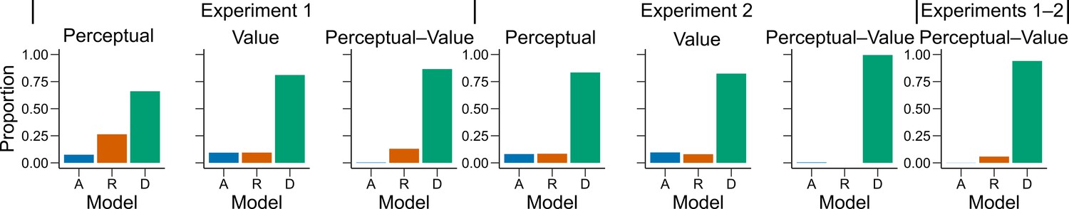
Behavioral results.

(a) Bars represent proportion of times an encoding rule (Accuracy [A, blue], Reward [R, red], DbS [D, green]) was selected by the Bayesian latent-mixture model based on the posterior estimates across participants. Each panel shows the data grouped for each and across experiments and experimental conditions (see titles on top of each panel). The results show that DbS was clearly the favored encoding rule. The latent vector $π$ posterior estimates are presented in Figure 4—figure supplement 4. (b) Difference in LOO and WAIC between the best model (DbS (D) in all cases) and the competing models: Accuracy (A), Reward (R) and Logarithmic (L) models. Each panel shows the data grouped for each and across experimental conditions and experiments (see titles on top of each panel). (c) Behavioral data (black, error bars represent SEM across participants) and model predictions based on fits to the empirical data. Data and model predictions are presented for both the perceptual (left panels) or value (right panels) conditions, and excluding (top panels) or including (bottom panels) choice history effects. Performance of data model predictions is presented as function of the sum of the number of dots in both clouds (left), the absolute difference between the number of dots in both clouds (middle) and the ratio of the number of dots in the most numerous cloud over the less numerous cloud (right). Results reveal a remarkable overlap of the behavioral data and predictions by DbS, thus confirming the quantitative results presented in panels a and b.

Figure 4—figure supplement 1

Download asset Open asset

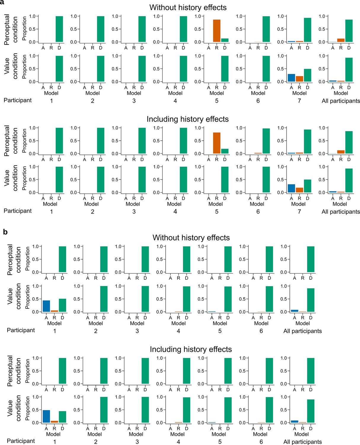
Latent mixture model fits for each participant.

Individual level fit of the latent mixture model excluding (top) or including (bottom) choice history effects for (a) Experiment 1 and (b) Experiment 2. The panels on the far right shows the average fit for all the participants of the given experiment. DbS is strongly favored for nearly all participants and clearly favored across participants, irrespective of the experimental condition. Including choice and correctness information of previous trials has minimal influence in the results of these analyses, which rules out the influence of these effects on the decision rule used by the participants.

Figure 4—figure supplement 2

Download asset Open asset

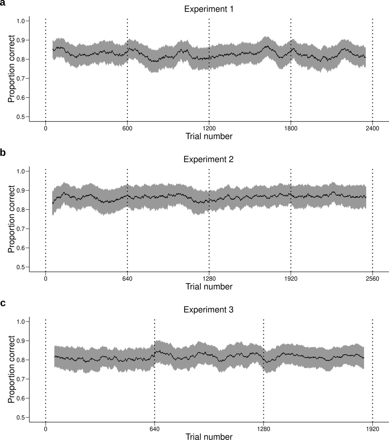
Performance across time.

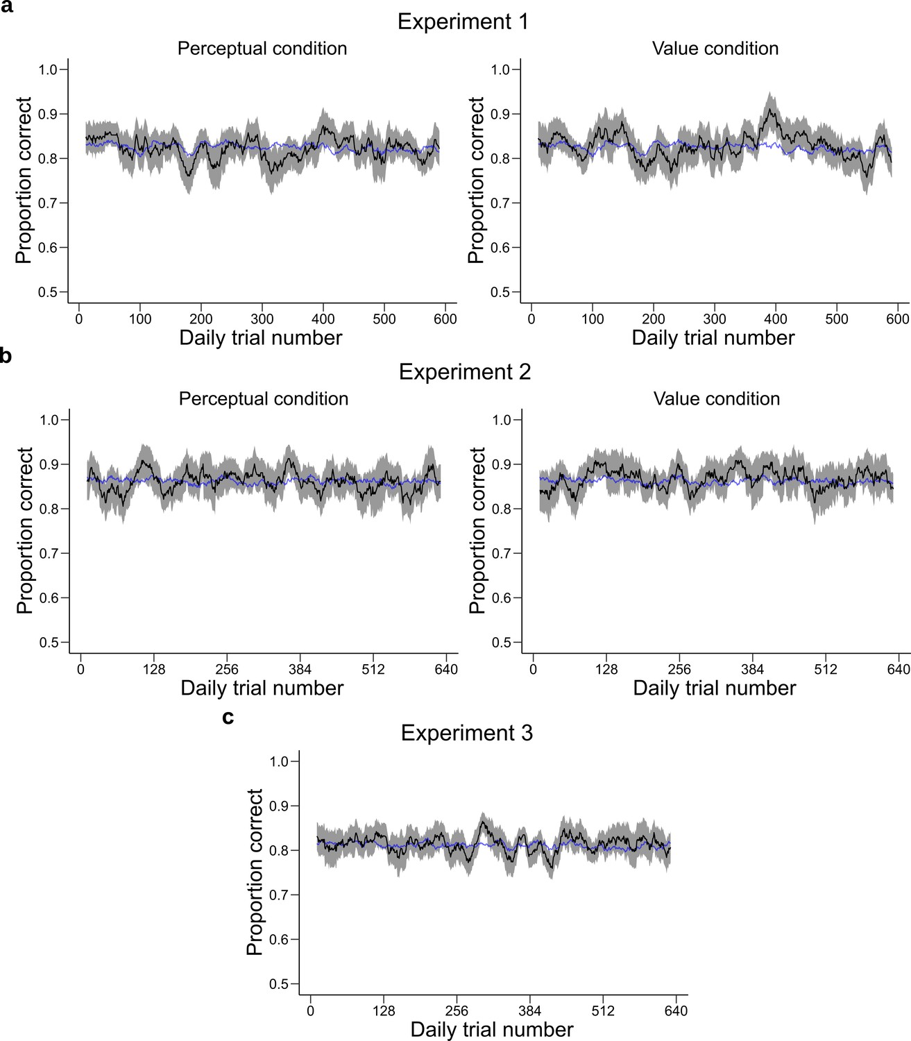
Behavioral performance (mean ± SEM across participants) averaged over a moving window of 100 trials for (a) Experiment 1, (b) Experiment 2 and (c) Experiment 3. Each daily session took place between two dotted vertical lines. The performance of the participants is stable during and between daily sessions. Therefore, the quantitative and qualitative results presented in the main text are not likely to be influenced by changes in performance over time.

Figure 4—figure supplement 3

Download asset Open asset

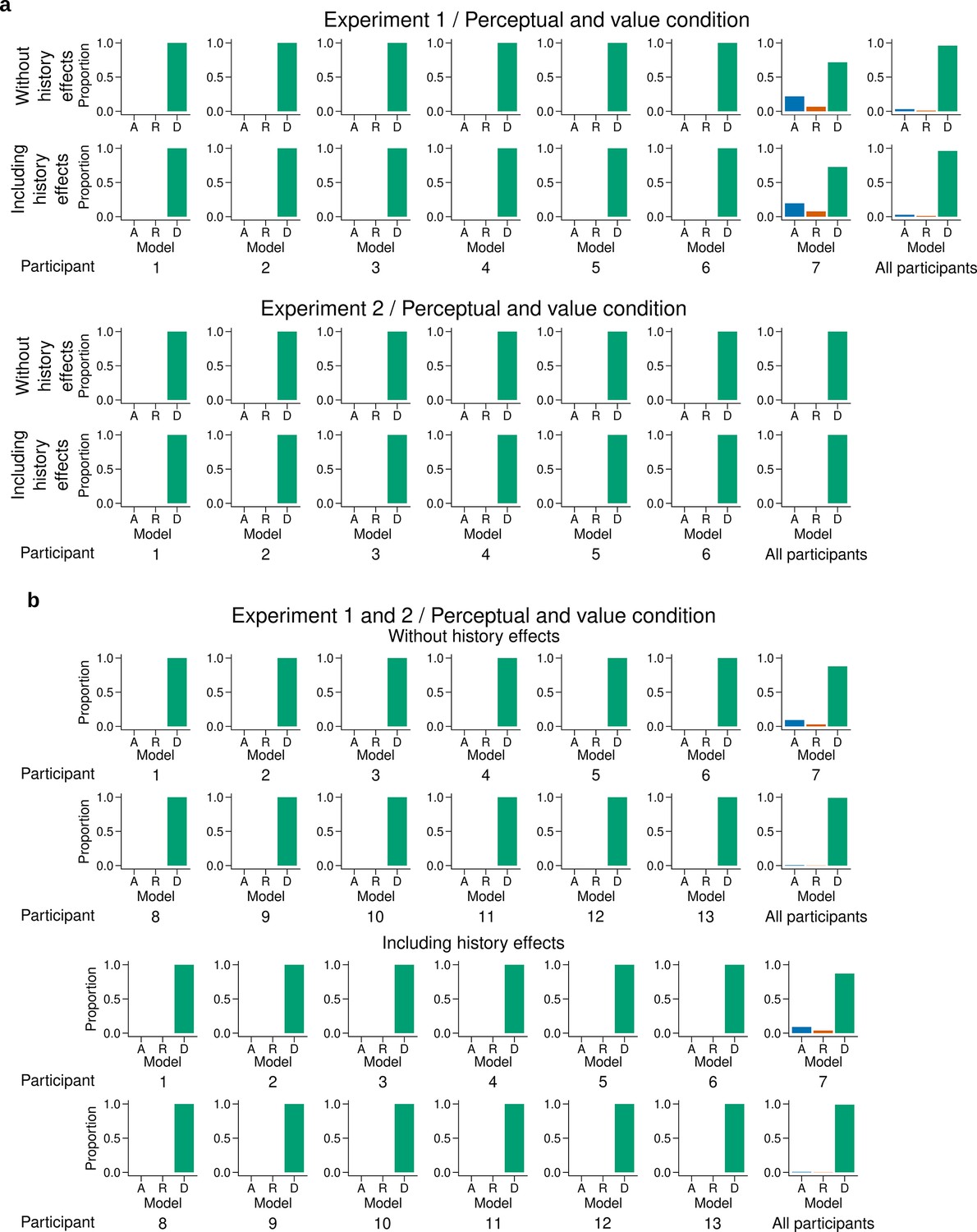
Individual level fit of the latent mixture model combining data across experiments and experimental conditions.

(a) Individual level fit of the latent mixture model combining data across both experimental conditions for Experiment 1 (top) and Experiment 2 (bottom). (b) Individual level fit of the latent mixture model combining data across both experimental conditions and both experiments. Each panel shows the results excluding (top) or including (bottom) choice history effects. The panels labeled 'All participants' show the average fit for all the participants of the given experiment. DbS is strongly favored irrespective of incentivized goals. Including the previous trial effects has minimal influence on these results.

Figure 4—figure supplement 4

Download asset Open asset

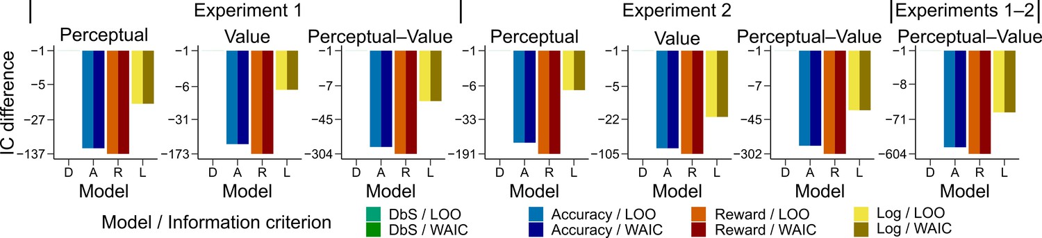
Model comparison based on leave-one-out cross-validation metrics.

Quantitative comparison of the models including choice and correctness effects of previous trials based on leave-one-out cross-validation metrics. Difference in LOO and WAIC between the best model (DbS (D) in all cases) and the competing models: Accuracy (A), Reward (R) and Logarithmic (L) models. Each panel shows the data grouped for each and across experiments and experimental conditions (see titles on top of each panel). Including the previous choice and correctness effects has only little influence on the results (compare with Figure 4b in main text). The DbS model provides the best fit to the behavioral data.

Figure 4—figure supplement 5

Download asset Open asset

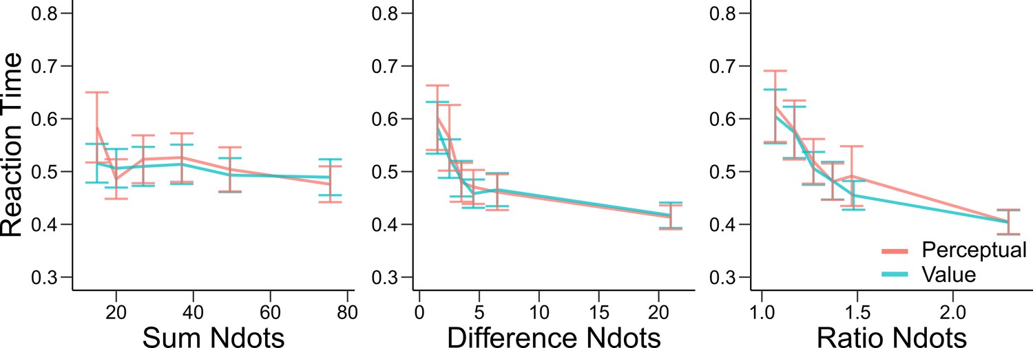
Reaction times are similar in the perceptual and value conditions.

Mean reaction times of participants in Experiments 1 and 2 in the perceptual (red) and value (blue) condition. Error bars represent SEM across participants. Reaction times are presented as a function of the sum of the number of dots in both clouds (left), the absolute difference between the number of dots in both clouds (middle) and the ratio of the number of dots in the most numerous cloud over the less numerous cloud (right). Non-parametric ANOVA tests revealed no significant differences in any of these behavioral assessments (all tests p>0.4).

Figure 4—figure supplement 6

Download asset Open asset

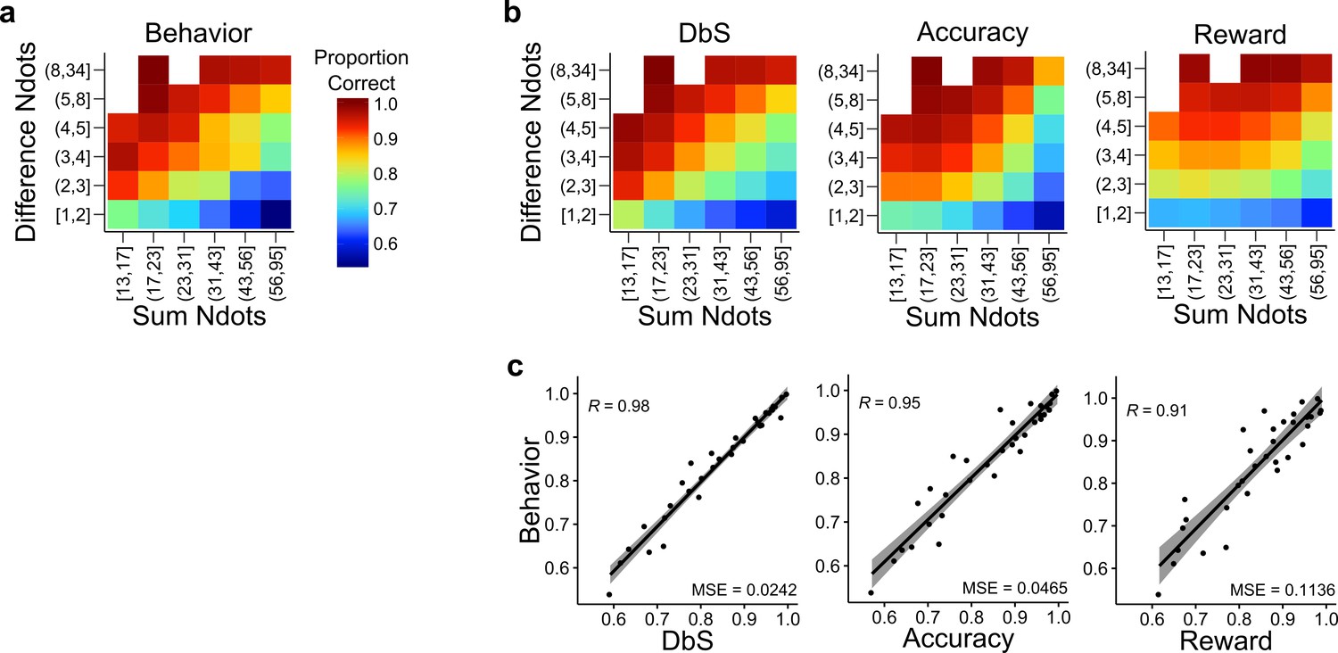
Behavior and model predictions as a function of sum and difference in dots.

(a) Average behavior in both conditions of Experiments 1 and 2 as a function of the sum of the number of dots in both clouds (Sum Ndots) and the absolute difference between the number of dots in both clouds (Difference Ndots). The data are binned as in Figure 4 but now expanded in two dimensions. (b) Predictions of each encoding rule model fit with only $n$ as a free parameter shown with the same scale as in a. (c) Linear regression between the behavior for each combination of Sum Ndots and Difference Ndots bins and the predictions of each model for the same bins. DbS captures best the changes in behavior across bins of sum and absolute difference of the number of dots in both clouds. This analysis should not be considered as a quantitative proof, but as a qualitative inspection of the results presented in Figure 4.

Figure 4—figure supplement 7

Download asset Open asset

Model fit for the first experimental condition of each participant.

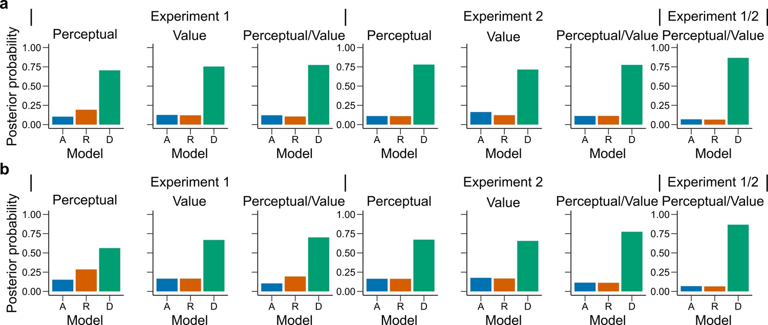
Similar as in Figure 4a, bars represent proportion of times an encoding rule (Accuracy [A, blue], Reward [R, red], DbS [D, green]) was selected by the Bayesian latent-mixture model based on the posterior estimates across participants. Each panel shows the data grouped for each experiment and experimental conditions (see titles on top of each panel). The latent-mixture model was only fit to the first condition that was carried out by each participant. As the participants did not know of the second condition before carrying it out, they could not adopt compromise strategies between the two objectives. Therefore, the fact that DbS is favored in the results is not an artifact of carrying out two different conditions in the same participants.

Figure 4—figure supplement 8

Download asset Open asset

Latent vector $π$ posterior estimates.

Bars represent the posterior distribution of the latent vector $π$ , with each bar representing an encoding rule (Accuracy (A, blue), Reward (R, red), DbS (D, green)). Results are presented for (a) all sessions and (b) only the first condition carried out by each participant. DbS is consistently the most likely encoding rule.

Figure 5 with 3 supplements

Download asset Open asset

Prior adaptation analyses.

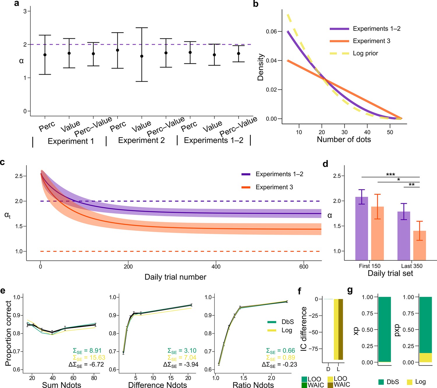
(a) Estimation of the shape parameter $α$ for the DbS model by grouping the data for each and across experimental conditions and experiments. Error bars represent the 95% highest density interval of the posterior estimate of $α$ at the population level. The dashed line shows the theoretical value of $α$ . (b) Theoretical prior distribution $f (v)$ in Experiments 1 and 2 ( $α = 2$ , purple) and 3 ( $α = 1$ , orange). The dashed line represents the value of $α$ of our prior parametrization that approximates the DbS and log discriminability models. (c) Posterior estimation of $α_{t}$ (Equation 18) as a function of the number of trials $t$ in each daily session for Experiments 1 and 2 (purple) and Experiment 3 (orange). The results reveal that, as expected, $α_{t}$ reaches a lower asymptotic value $δ$ . Error bars represent ± SD of 3000 simulated $α_{t}$ values drawn from the posterior estimates of the HBM (see Materials and methods). (d) Model fit to the first 150 and last 350 trials of each daily session. The $α$ parameter was allowed to vary between the first and last sets of daily trials and between Experiments 1–2 and Experiment 3. In Experiment 3, $α$ is lower in the last set of trials compared to the first set of trials ( $P_{MCMC} = 0.013$ ). In addition, $α$ for the last trials is lower for Experiment 3 than for Experiments 1–2 ( $P_{MCMC} = 0.006$ ). This confirms that the results presented in panel c are not artifacts of the adaptation parametrization assumed for $α$ . Error bars represent ± SD of the posterior chains of the corresponding parameter. (*P<0.05, **P<0.01, and ***P<0.001). (e) Behavioral data (black) and model fit predictions of the DbS (green) and Log (yellow) models. Performance of each model as a function of the sum of the number of dots in both clouds (left), the absolute difference between the number of dots in both clouds (middle) and the ratio of the number of dots in the most numerous cloud over the less numerous cloud (right). Error bars represent SEM (f) Difference in LOO and WAIC between the best fitting DbS (D) and logarithmic encoding (Log) model. (g) Population exceedance probabilities (xp, left) and protected exceedance probabilities (pxp, right) for DbS (green) vs Log (yellow) of a Bayesian model selection analysis (Stephan et al., 2009): ${xp}_{DbS} = 0.99$ , ${pxp}_{DbS} = 0.87$ . These results provide a clear indication that the adaptive DbS explains the data better than the Log model.

Figure 5—figure supplement 1

Download asset Open asset

Performance across trial experience.

These plots represent the performance of the participants as a function of the number of trials they have experienced during the session. The performance of the participants (black, shaded area represents ± SEM across participants) was averaged over a moving window of 21 trials and is shown for Experiment 1 (a) Experiment 2 (b) and Experiment 3 (c). The blue line represents the performance predicted by the $α$ -adaptation model using the same moving window average. The model provides a good fit to average performance.

Figure 5—figure supplement 2

Download asset Open asset

Quantitative and dynamical analysis of adaptation over time.

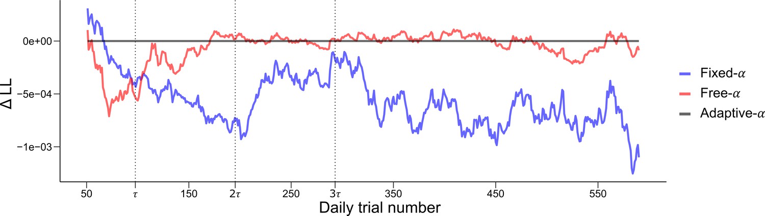
To further investigate the adaptation of the prior, we fit three models of varying complexity to the data of Experiments 1, 2 and 3. The Fixed- $α$ model (blue) is defined with a fixed $α = 2$ . The Free- $α$ model (red) allows the $α$ parameter to vary across participants but is kept constant across time. The Adaptative- $α$ corresponds to the model presented in Figure 5 where the prior adapts as the participants gains experience with the experimental distribution of dots. To allow a fair comparison with the Free- $α$ model, the $δ$ parameter, corresponding to the asymptotic value of the prior, was free to vary across participants. The log-likelihood of each model on each trial were averaged over a moving window of 100 trials and the log-likelihood of the Adaptative- $α$ model was subtracted for comparison. Vertical dashed lines represent 1, 2 and 3 times $τ$ , where $τ$ controls the rate of adaptation in the Adaptative- $α$ model. The Adaptative- $α$ model provides a better fit for the first trials (until around $2 τ$ ), these trials correspond to the adaptation period where the $α$ parameter is changing in the Adaptative- $α$ model (see Figure 5). After this point the Adaptative- $α$ and Free- $α$ models provide a similar fit. This is to be expected as the function controlling the decay of $α$ reaches its asymptotic value, leaving the two model virtually identical. The Fixed- $α$ provides overall a worse fit, except for the early trials.

Figure 5—figure supplement 3

Download asset Open asset

Model fits for the beginning and end of each session without parametric assumptions.

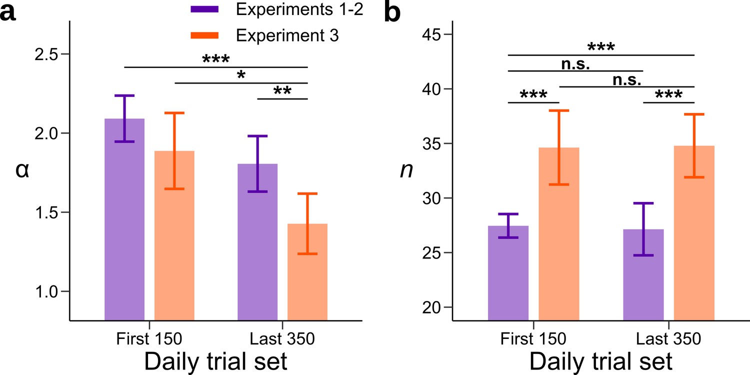
A model was fitted to the first 150 and last 350 trials of each daily session. The prior parameter $α$ and the number of neural resources $n$ were allowed to vary between the first and last sets of daily trials and between Experiments 1–2 (purple) and Experiment 3 (orange). (a) Each bar represents the mean value of the $α$ parameter for a combination of experiments and set of daily trials. In Experiment 3, $α$ is lower in the last set of trials compared to the first set of trials. In addition, the value of $α$ for Experiment 3 is lower than for Experiments 1–2 in the last set of daily trials. (b) Each bar represents the value of the neural resource parameter $n$ for a combination of experiments and set of daily trials. The neural resources parameter $n$ in Experiment 3 is larger than in Experiments 1–2. However, there is no change in the neural resource parameter across the session. This suggests that the adaptation process is not an artifact of changes in the neural resource parameter, which could for example change with the engagement of the participants across the session. Significance between parameters was computed by subtracting the chain with the largest mean to the other one and measuring the proportion of values that fall below 0 (n.s. P < 0.05, *P<0.05, **P<0.01, and ***P<0.001). Error bars represent ± SD of the posterior chains of the corresponding parameter.

Appendix 4—figure 1

Download asset Open asset

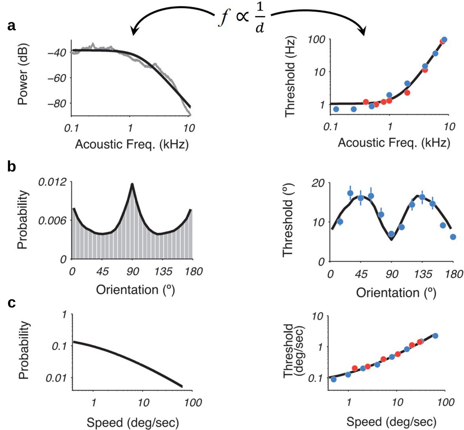
Recently, it was shown that using an efficiency principle for encoding sensory variables, based on population of noisy neurons, it was possible to obtain an explicit relationship between the statistical properties of the environment (the prior) and perceptual discriminability (Ganguli and Simoncelli, 2016).

The theoretical relation states that discriminability should be inversely proportional to the density of the prior distribution. Interestingly, this relationship holds across several sensory modalities such as (a) acoustic frequency, (b) local orientation, (c) speed (figure adapted with permission from the authors Ganguli and Simoncelli, 2016). Here, we investigate whether this particular relation also emerges in our efficient sampling framework.

Appendix 7—figure 1

Download asset Open asset

Tables

Table 1

Resource parameter $n$ fits.

Fits of the resource parameter for the Accuracy, Reward and Decision by Sampling (DbS) models including data across experiments and conditions (perceptual (P) or value (V)) either including or ignoring choice history effects. The values represent the mean ± SD of the posterior distributions at the population level for parameter $n$ . Note that Reward and in particular the DbS encoding models require a higher number of resources than the Accuracy model, which is coherent with the fact that the Accuracy model allocates its resources to maximize efficiency, therefore reducing the number of resources needed to reach a given accuracy. DbS has the highest values of $n$ because it is the most inefficient model.

			Model
Experiment	Condition	History effects	n_Accuracy	n_Reward	n_DbS
1	V	not included	15.24 ± 3.09	17.54 ± 3.98	24.40 ± 5.16
2	V	not included	22.48 ± 2.43	27.58 ± 3.81	35.40 ± 3.44
1	P	not included	15.19 ± 3.99	17.84 ± 4.85	24.64 ± 6.59
2	P	not included	20.99 ± 1.59	24.22 ± 1.93	33.54 ± 2.45
1	P/V	not included	15.33 ± 3.41	17.25 ± 4.45	24.15 ± 5.75
2	P/V	not included	21.30 ± 0.96	25.27 ± 1.99	33.90 ± 1.51
1/2	V	not included	18.56 ± 2.04	22.05 ± 2.73	29.52 ± 3.25
1/2	P	not included	17.91 ± 2.09	20.66 ± 2.59	28.62 ± 3.51
1/2	P/V	not included	17.93 ± 1.87	21.03 ± 2.46	28.58 ± 3.04
1	V	included	15.50 ± 3.13	17.50 ± 3.91	24.68 ± 5.08
2	V	included	22.92 ± 2.37	28.07 ± 3.73	36.18 ± 2.91
1	P	included	15.41 ± 3.81	17.96 ± 4.88	24.70 ± 6.62
2	P	included	21.57 ± 1.71	24.88 ± 2.17	34.37 ± 2.93
1	P/V	included	15.16 ± 3.55	17.43 ± 4.39	24.30 ± 5.94
2	P/V	included	21.80 ± 0.92	25.81 ± 1.86	34.60 ± 1.40
1/2	V	included	18.86 ± 2.07	22.48 ± 2.75	29.85 ± 3.17
1/2	P	included	18.15 ± 2.17	21.11 ± 2.72	29.01 ± 3.47
1/2	P/V	included	18.22 ± 1.93	21.34 ± 2.50	29.12 ± 3.12