An electrophysiological marker of arousal level in humans
- Helen Wills Neuroscience Institute, University of California, Berkeley, United States
- Department of Anesthesiology and Intensive Care Medicine, University Medical Center Tuebingen, Germany
- Hertie-Institute for Clinical Brain Research, Germany
- Department of Neurology and Epileptology, University Medical Center Tuebingen, Germany
- Department of Psychiatry and Human Behavior, University of California, Irvine, United States
- Department of Anesthesiology, University of Oslo Medical Center, Norway
- Department of Neurology, University of California, Irvine, United States
- Department of Psychology, University of California, Berkeley, United States
- Department of Neurosurgery, University of Oslo Medical Center, Norway
Figures
Figure 1 with 4 supplements
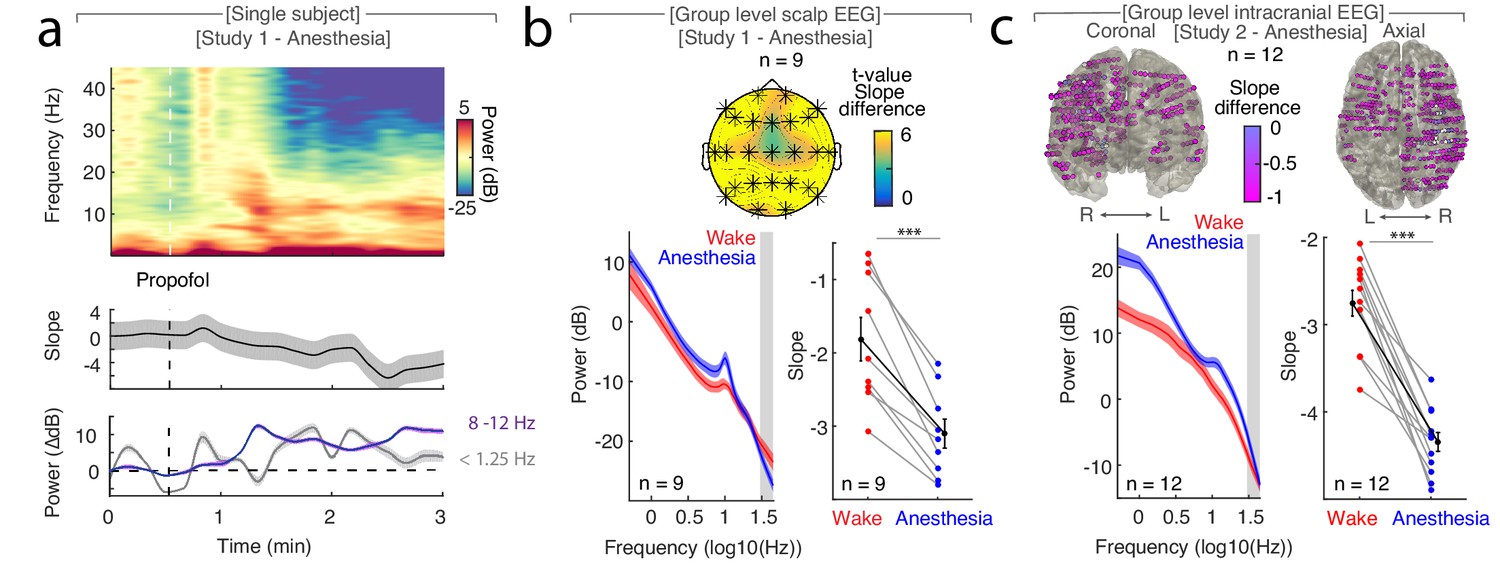
The spectral slope tracks changes in arousal level under general anesthesia with propofol.
(a) Time-resolved average of three frontal EEG channels (F3, Fz, F4) during anesthesia. Upper panel: Time-frequency decomposition. Dotted white line: Induction with propofol. Middle: Spectral slope (black; mean ± SEM). Lower panel: Slow frequency (<1.25 Hz; gray) and alpha (8–12 Hz; purple) baseline-corrected power (mean ± SEM). Note, elevated slow frequency activity is already present during wakefulness. While alpha frequency activity is steadily increasing in the first minutes of anesthesia, slow frequency activity exhibits a waxing and waning pattern which may reflect the premedication with a sedative. (b) Anesthesia in scalp EEG (n = 9). Upper panel: Spatial extent of spectral slope difference. Cluster permutation test: *p<0.05. Lower panel: Left - Power spectra (mean ± SEM); Right – Spectral slope. Wakefulness (red), anesthesia (blue) and grand average (black; all mean ± SEM). Permutation t-test: ***p<0.001. (c) Anesthesia in intracranial recordings (n = 12). Upper panel: Left – coronal, right – axial view of intracranial channels that followed (magenta) or did not follow (white) the EEG pattern of a lower slope during anesthesia compared to wakefulness. Lower panel: Left – Power spectra; Right – Spectral slope. Wakefulness (red), anesthesia (blue) and grand average (black; mean ± SEM). Permutation t-test: ***p<0.001.
Figure 1—figure supplement 1

Coverage in intracranial subjects.
(a) Anesthesia intracranial EEG – Grid, strip and SEEG contacts of all subjects (n = 12) plotted on a Montreal Neurological Institute (MNI) brain. Right (R), left (L), ventral (V), dorsal (D). (b) Sleep intracranial EEG – Grid and SEEG contacts of all subjects (n = 10) plotted on MNI brain. Right (R), left (L), ventral (V), dorsal (D).
Figure 1—figure supplement 2

Differences in spectral slope under general anesthesia and in sleep in cortical recording sites.
(a), All grid and strip contacts of 4 patients plotted on MNI brain. Electrodes that followed the pattern of a more negative slope under anesthesia than in waking are colored in purple to magenta. Electrodes that did not show the pattern are depicted in white. Right (R), left (L), ventral (V), dorsal (D). (b) All grid and strip contacts of 3 patients plotted on MNI brain. Electrodes that followed the pattern of a more negative slope in NREM stage three sleep than in waking are colored purple to magenta. Electrodes that did not show the pattern are depicted in white. Ventral (V), dorsal (D). (c) All grid and strip contacts of 3 patients plotted on MNI brain. Electrodes that followed the pattern of a more negative slope in REM sleep than in waking are colored in purple to magenta. Electrodes that did not show the pattern are depicted in white. Ventral (V), dorsal (D).
Figure 1—figure supplement 3
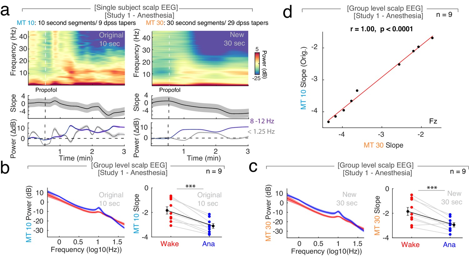
The influence of segment length and number of tapers on spectral slope estimation under general anesthesia with propofol.
(a) Single subject example at EEG electrode Fz during induction of propofol anesthesia. Left panels – Original observation: 10 s segments (nine discrete prolate spheroidal sequences (dpss) tapers). Right panels – New observation: 30 s segments (29 dpss tapers). Upper panels - Multitapered (MT) time-frequency decomposition. Middle panels – Time-resolved spectral slope (gray; mean ± SEM). Lower panels – Slow oscillation (<1.25 Hz; gray) and alpha power (8–12 Hz; purple; mean ± SEM). Dotted lines: Induction with propofol. Note the temporal smoothing with 30 s compared to 10 s segments. MT power spectra in log-log space (left panels; mean ± SEM) and 1/f slope (right panels; black - mean ± SEM) in wakefulness (Wake - red) and under general anesthesia with propofol (Ana - blue) in scalp EEG (n = 9; averaged across all channels). (b) Original observation: Power spectra and slopes calculated in 10 s segments (blue; nine dpss tapers). ***p<0.001. (c) New observation: Power spectra and slopes calculated in 30 s segments (orange; 29 dpss tapers). ***p<0.001. (d) At electrode Fz, the 1/f slope values derived from 10 and 30 s segments in anesthesia scalp EEG are strongly correlated (n = 9; r = 1.00, p<0.0001).
Figure 1—figure supplement 4
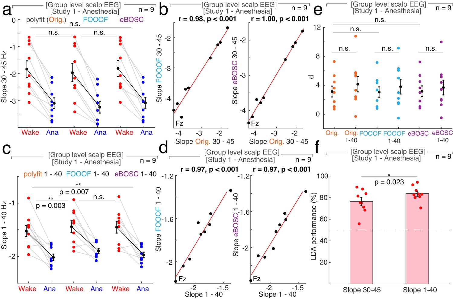
The influence of different fit algorithms and fit lengths on spectral slope estimation in general anesthesia with propofol.
Spectral slopes were calculated using either the original (30 to 45 Hz; panels a - c) or a wider frequency range (1 to 40 Hz; panels d - f). (a) 1/f spectral slopes in wakefulness (Wake, red) and under anesthesia (Ana, blue) using the original polyfit (Orig., orange), FOOOF (blue) or eBOSC (purple) algorithm between 30 and 45 Hz (n = 9, averaged across electrodes). Paired t-tests (uncorrected): Orig.-FOOOF: p=0.082, t8 = 1.99, d = 0.18; Orig.- eBOSC: p=0.369, t8 = −0.95, d = −0.03, FOOOF - eBOSC: p=0.118, t8 = −1.75, d = −0.21. n.s. – not significant. (b) At Fz, 1/f slopes from original polyfit (Orig., orange) and FOOOF (blue; left panel: r = 0.98, p<0.001) and original and eBOSC (purple; right panel: r = 1.00, p<0.001) between 30 and 45 Hz are strongly correlated. (c) 1/f spectral slopes in wakefulness (Wake, red) and under anesthesia (Ana, blue) using the original polyfit (Orig., orange), FOOOF (blue) or eBOSC (purple) algorithm between 1 and 40 Hz (n = 9, averaged across electrodes). Paired t-tests (uncorrected): Orig.-FOOOF: p=0.003, t8 = −4.29, d = −0.49; Orig.- eBOSC: p=0.007, t8 = −3.60, d = −0.29, FOOOF - eBOSC: p=0.112, t8 = 1.78, d = 0.21. n.s. – not significant. **p<0.01. (d) At Fz, 1/f slopes from original polyfit (Orig., orange) and FOOOF (blue, left panel: r = 0.97, p<0.001) and from original and eBOSC (purple, right panel: r = 0.97, p<0.001) between 1 and 40 Hz are strongly correlated. (e) Comparison of effect size (Cohen’s d) between spectral slopes in wakefulness and anesthesia (n = 9) result in no significant difference between fits in all three fitting algorithms (original – orange, FOOOF – blue, eBOSC – purple). Permutation t-tests: Orig.30-45 - Orig.1-40: p=0.773, obs. t8 = −0.84, d = −0.37; fooof30-45 – fooof1-40: p=0.737, obs. t8 = −0.63, d = −0.28; eBOSC30-45 – eBOSC1-40: p=0.672, obs. t8 = −0.47, d = −0.20; Orig.30-45 -fooof30-45: p=0.242, obs. t8 = 0.72, d = 0.03; Orig.30-45-eBOSC30-45: p=0.098, obs. t8 = −1.40, d = −0.01; fooof30-45- eBOSC30-45: p=0.173, obs. t8 = −1.01, d = −0.04. n.s. – not significant. (f) Linear Discriminant Analysis (LDA) using either the spectral slope between 30 and 45 or 1 and 40 Hz (n = 9). Performances were logit-transformed and averaged across channels before comparison. The 1 to 40 Hz performed better than 30 to 45 Hz (Slope30-45: 76.56 ± 3.56% (mean ± SEM), Slope1-40: 83.75 ± 2.31%; permutation t-test: p=0.023, obs. t8 = -2.49, d = -0.83) possibly by including the strong alpha oscillation that occurs under propofol anesthesia (compare Figure 1). *p<0.05.
Figure 2 with 11 supplements
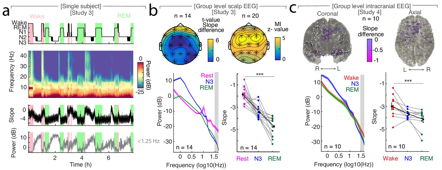
The spectral slope tracks changes of arousal level in sleep.
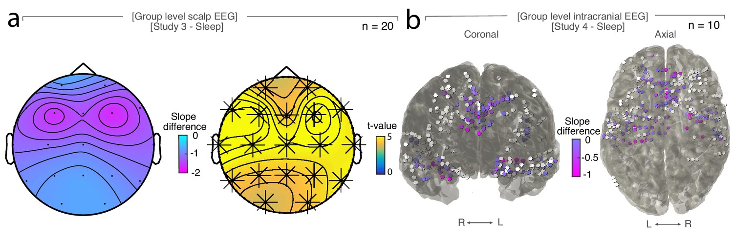
(a) Time-resolved average of three frontal EEG channels (F3, Fz, F4) during a night of sleep. Upper panel: Expert-scored hypnogram (black), wake (pink), REM (light green). Upper middle: Time-frequency decomposition. Lower middle: Spectral slope (black; mean ± SEM). Lower panel: Slow frequency (<1.25 Hz) power (gray; mean ± SEM). (b) Sleep in scalp EEG. Upper panel: Left: Slope difference between sleep and rest (n = 14). Cluster permutation test: *p<0.05. Right: Mutual Information (MI) between the time-resolved slope and hypnogram (n = 20). Cluster permutation test against surrogate distribution created by random block swapping: *p<0.05. Lower panel: Left - Power spectra (n = 14; mean ± SEM); Right – Spectral slope (n = 14). Rest (magenta), NREM stage 3 (blue), REM sleep (green) and grand average (black; mean ± SEM). Repeated measures ANOVA permutation test: ***p<0.001. (c) Sleep in intracranial EEG (n = 10). Upper panel: Left – coronal, right – axial view of intracranial channels that followed (magenta) or did not follow (white) the EEG pattern of a lower slope during sleep (REM/N3). Lower panel: Left – Power spectra (mean ± SEM); Right – Spectral slope of simultaneous EEG recordings (Fz, Cz, C3, C4, Oz). Wakefulness (red), NREM stage 3 (N3; blue), REM sleep (green) and grand average (black; mean ± SEM). Repeated measures ANOVA permutation test: ***p<0.001.
Figure 2—figure supplement 1
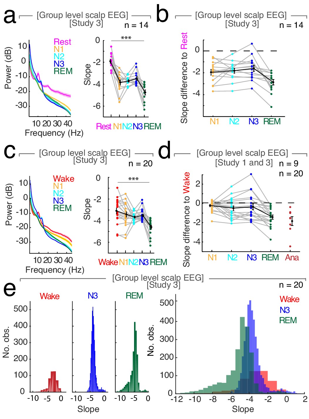
Relative changes of spectral slope reliably differentiate between wakefulness, sleep and general anesthesia.
(a) Left – Mean power spectra (± SEM) averaged across all channels and subjects (n = 14) during rest recording of 5 min eyes closed recorded before sleep compared to all sleep stages. Right – Slope values. Mean ± SEM in black. Repeated measures ANOVA: ***p<0.001, F2.54, 33.02 = 38.02, dRest-Sleep = 3.52. Post-hoc t-tests: pRest-N2 <0.001; t13 = 7.97; d = 3.31; pRest-N3 <0.001; t13 = 5.69; d = 2.49; pRest-REM <0.001; t13 = 11.67; d = 3.71; pN3-REM < 0.0001; t13 = 4.44; d = 1.70. (b) Slope differences of all sleep stages to rest (n = 14). Mean ± SEM in black. (c) Left - Mean power spectra (± SEM) averaged across all channel and subjects (n = 20) during wakefulness and all sleep stages. Right - Slope values. Mean ± SEM in black. Repeated measures ANOVA: ***p<0.001, F1.86, 33.49 = 13.39, dWake-Sleep = 0.79. Post-hoc t-tests: pWake-N2 = 0.029, t18 = 2.36, d = 0.69; pWake-N3 = 0.19; t18 = 1.34; d = 0.48; pWake-REM <0.0001; t18 = 6.83; d = 1.58; pN3-REM < 0.0001; t19 = 5.12; d = 1.66. (d) Slope difference of all sleep stages to all wake trials (n = 20) and anesthesia to wake trials before anesthesia (n = 8). Mean ± SEM in black. (e) Histogram of slope values pooled across all participants (n = 20). Wakefulness (red), N3 (blue), REM (green). Left: Separated values of each sleep stage. Right: All three sleep stages within one plot.
Figure 2—figure supplement 2

The spectral slope is not confounded by muscle activity.
(a) Laplacian reference (n = 20). Upper topoplot: Cluster permutation test of Spearman rank correlation between hypnogram and time-resolved slope: *p<0.05. Lower topoplot: Mututal Information between slope and hypnogram. Statistics with random block swapping: *p<0.05. (b) Cluster permutation test of Spearman rank correlation between hypnogram and time-resolved slope with electromyography (EMG) slope partialled out (n = 20): *p<0.05. (c) Hypnogram of a single subject (upper panel), time-resolved slope averaged over EEG channels F3, Fz and F4 (middle panel), time-resolved slope of EMG signal averaged over three EMG channels (lower panel). (d) EMG signal on group level across a full night (n = 20). Left: Power spectra of EMG (mean ± SEM). Right: Slope of EMG in wakefulness (red), NREM stage 3 (N3; blue), REM (green), grand average (black, mean ± SEM). (e) R2 of Spearman rank correlations averaged across all channels between hypnogram and slope (magenta), EMG slope (cyan) and the slope with the EMG slope partialled out (yellow, all mean ± SEM). The correlation of hypnogram - slope and hypnogram - EMG slope is significantly different (paired t-test: p=0.0059, t19 = 3.10). Furthermore, we utilized the LDA classification approach to test if the spectral slope outperforms the EMG slope for state discrimination (n = 19; one patient excluded due to noisy wake trials). We found that the spectral slope performed significantly better at distinguishing all three states (slope: 58.09 ± 2.35%, EMG slope: 46.03 ± 2.12%; chance 33%; paired t-test: p<0.001, t18 = 4.19, d = 1.24). Likewise, the slope was better at discriminating only wake and REM (slope: 76.32 ± 3.61%, EMG slope: 64.89 ± 2.24%; chance 50%; paired t-test: p=0.008, t18 = 3.03, d = 0.89).
Figure 2—figure supplement 3

Anatomical distribution of sleep dependent spectral slope modulation in scalp EEG.
(a) Sleep in intracranial study (n = 10). Upper panel: Left – coronal, right – axial view of intracranial channels that followed the EEG pattern of a lower slope during sleep (REM/NREM 3) compared to wakefulness. Color coded from black – no difference to yellow – strong difference. Note the lighter colored electrodes in medial prefrontal and medial temporal lobe areas. (b) Delta (Δ) slope between wakefulness and sleep source-interpolated on a standard template brain in MNI space with an LCMV beamformer (n = 19; one patient had to be excluded due to insufficient wake trials). Upper row – Sagittal views of right, lower row – sagittal view of left hemisphere. Color coded from black – no difference to yellow – strong difference. Note the lighter colored areas in medial prefrontal areas. V – ventral, D – dorsal. (c) Upper row - Regions of interest (ROI) source-interpolated on to a template brain in MNI space. Medial prefrontal cortex (mPFC) in red, dorso-lateral prefrontal cortex (dlPFC) in blue. Lower row - Delta (Δ) slope between wakefulness and sleep in mPFC and dlPFC. Only mPFC shows a significant sleep-dependent slope modulation (permutation t-test vs. zero: pmPFC = 0.018, pdlPFC = 0.074; permutation t-test between ROIs: pmPFC-dlPFC: p=0.036). *p<0.05. n.s. – not significant.
Figure 2—figure supplement 4
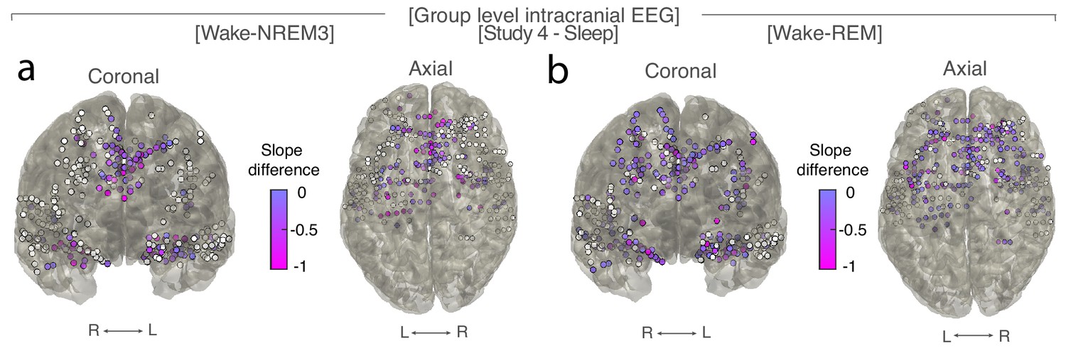
Differences of spectral slope in intracranial electrodes between waking and NREM sleep stage three or REM sleep (n = 10).
(a) Left – coronal, right – axial view of electrodes that followed the observed EEG pattern with a more negative slope in NREM sleep stage three than waking (magenta). Electrodes that did not show the pattern are depicted in white. Right (R), left (L). (b) Left – coronal, right – axial view of electrodes that followed observed EEG pattern with a more negative slope for REM sleep than in waking (magenta). Electrodes that did not show the pattern are depicted in white. Right (R), left (L).
Figure 2—figure supplement 5
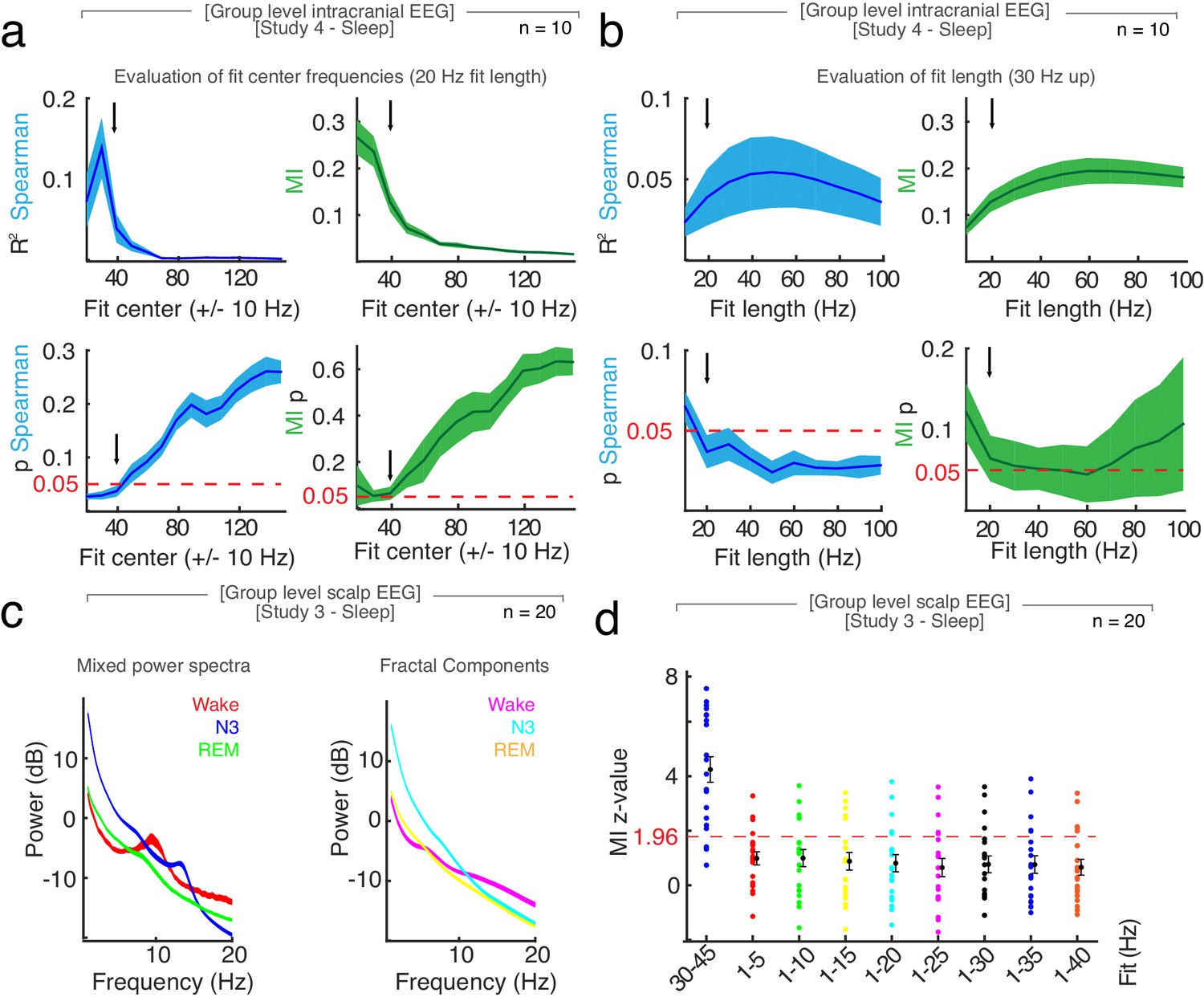
Evaluation of different slope fit settings in intracranial sleep.
(a) Fit center: Spearman rank correlation (blue, left panels) and Mutual Information (MI; green, right panels) between slope and hypnogram with different slope fits with center frequencies from 20 to 150 ± 10 Hz with SEM in intracranial data during sleep (n = 10). Upper left panel – R2 and lower left panel – p-value of Spearman rank correlation (blue). Upper right panel – MI and lower right panel – p-value of original MI observation tested against a surrogate MI distribution created by random block swapping (green). Red dotted lines for a p-value of 0.05. Black arrow indicates used center frequency of 40 Hz (30 to 50 Hz). (b) Fit length: Spearman rank correlation (blue, left panels) and Mutual Information (MI; green, right panels) with different slope fit lengths from 30 to 40 Hz up to 30 to 130 Hz (10 to 100 Hz fit length) with SEM in intracranial data during sleep (n = 10). Upper left panel – R2 and lower left panel – p-value of Spearman rank correlation (blue). Upper right panel – MI and lower right panel – p-value of original MI observation tested against a surrogate MI distribution created by random block swapping (green). Red dotted line for a p value of 0.05. Black arrow indicates used fit length for this study (20 Hz; 30 to 50 Hz). (c) Mixed (left) and fractal component (right) of power spectra in scalp EEG (n = 20) after IRASA. (d) Z-value of surrogate distribution (random block swapping) of Mutual Information (MI) between slope and hypnogram using the original (blue, 30 to 45 Hz) and different slope fits to fractal component (obtained by IRASA) in lower frequencies (scalp EEG, n = 20). Note that a z = 1.96 reflects an uncorrected two-tailed p-value of 0.05, while a z-score of >2.8 indicates a Bonferroni-corrected significant p-value (p<0.05/19 channels=0.0026).
Figure 2—figure supplement 6
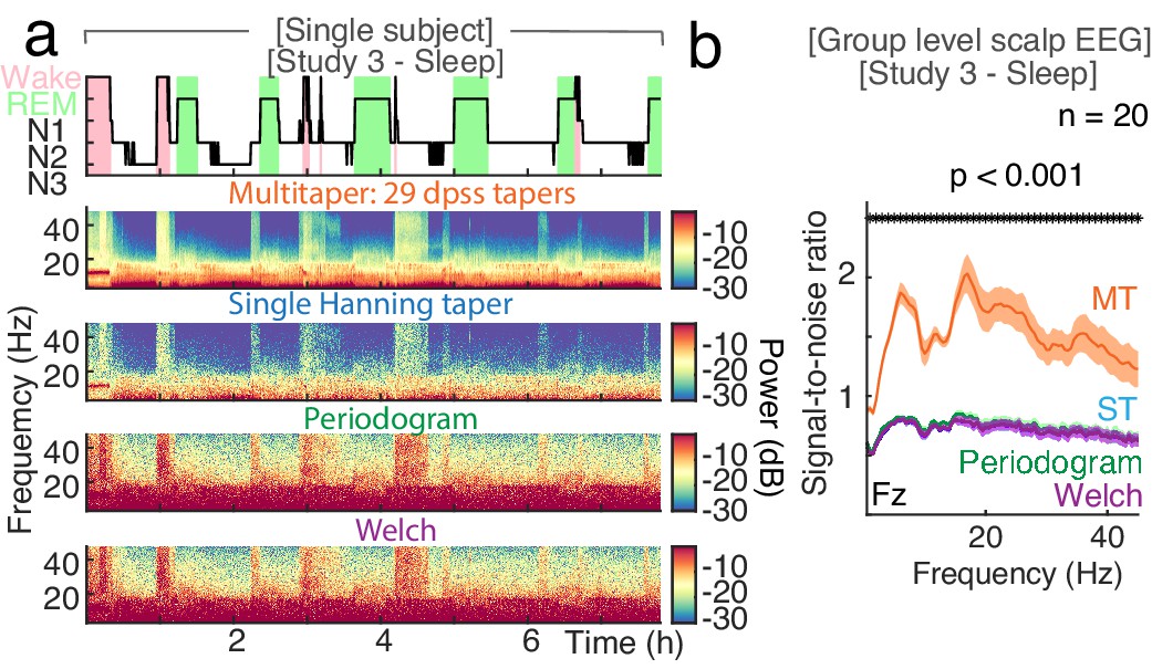
The influence of different power calculations on signal-to-noise ratio during sleep.
(a) Single subject example of time-resolved average of three frontal EEG channels (F3, Fz, F4) during a night of sleep. Upper panel: Expert-scored hypnogram (black), wake (pink), REM (light green). Upper middle panel – Time-frequency decomposition using the original Multitaper approach (orange) with 29 discrete prolate spheroidal sequences (dpss) tapers. Middle panel - Time-frequency decomposition using a single Hanning taper (blue). Lower middle panel - Time-frequency decomposition using a Periodogram (green). Lower panel - Time-frequency decomposition using Welch’s method with no overlap and a single taper (purple). Note, the visually smoother resolution of the multi-taper approach in comparison to the other time-frequency decompositions. (b) The Multitaper approach (MT, orange) had a significantly better signal-to-noise ratio (mean divided by standard deviation) at electrode Fz than the other approaches (single taper (ST, blue), Periodogram (green) and Welch’s method (purple); n = 20). This was true for all frequencies tested (0.5 to 45 Hz; cluster permutation test p<0.001). *p<0.05.
Figure 2—figure supplement 7
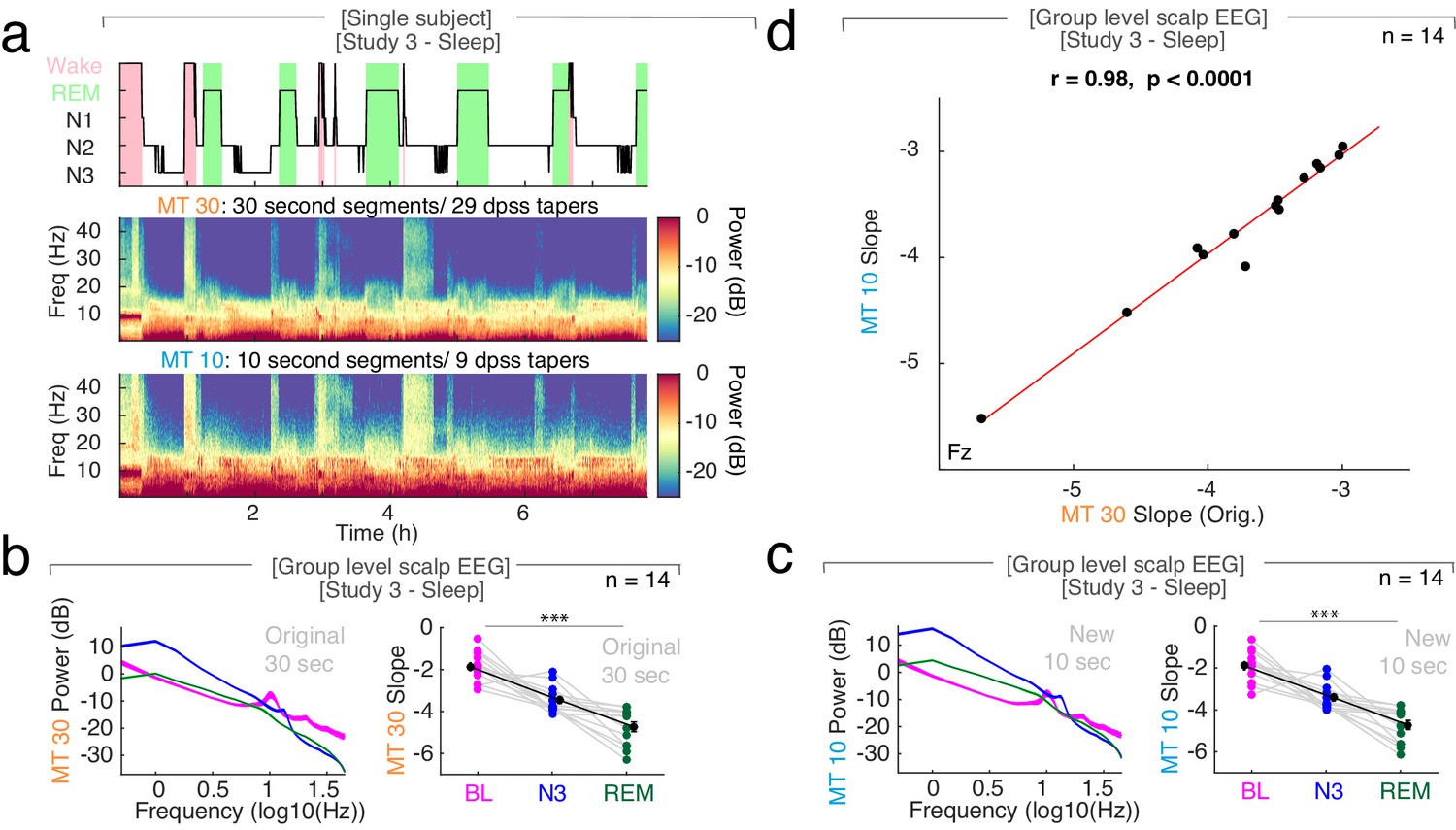
The influence of segment length and number of tapers on spectral slope estimation in sleep.
(a) Single subject example at EEG electrode Fz during a full night of sleep. Upper panel – Technician scored hypnogram. Wake periods highlighted in pink, REM in green. Middle Panel - Original observation: Multitapered (MT) time-frequency decomposition with 30 s segments (29 dpss tapers). Lower panel – New observation: MT time-frequency decomposition with 10 s segments (nine dpss tapers). MT Power spectra in log-log space (left panels; mean ± SEM) and 1/f slope (right panels; black - mean ± SEM) during baseline rest (BL - magenta), in NREM sleep stage 3 (N3 - blue) and REM sleep (REM - green) in scalp EEG (n = 14; averaged across all channels). (b) Original observation: Power spectra and slopes calculated in 30 s segments (orange; 29 dpss tapers). ***p<0.001. (c) New observation: Power spectra and slopes calculated in 10 s segments (blue; nine dpss tapers). ***p<0.001. (d) At electrode Fz, the 1/f slopes derived from 30 and 10 s segments in sleep scalp EEG are strongly correlated (n = 14; r = 0.95, p<0.0001).
Figure 2—figure supplement 8
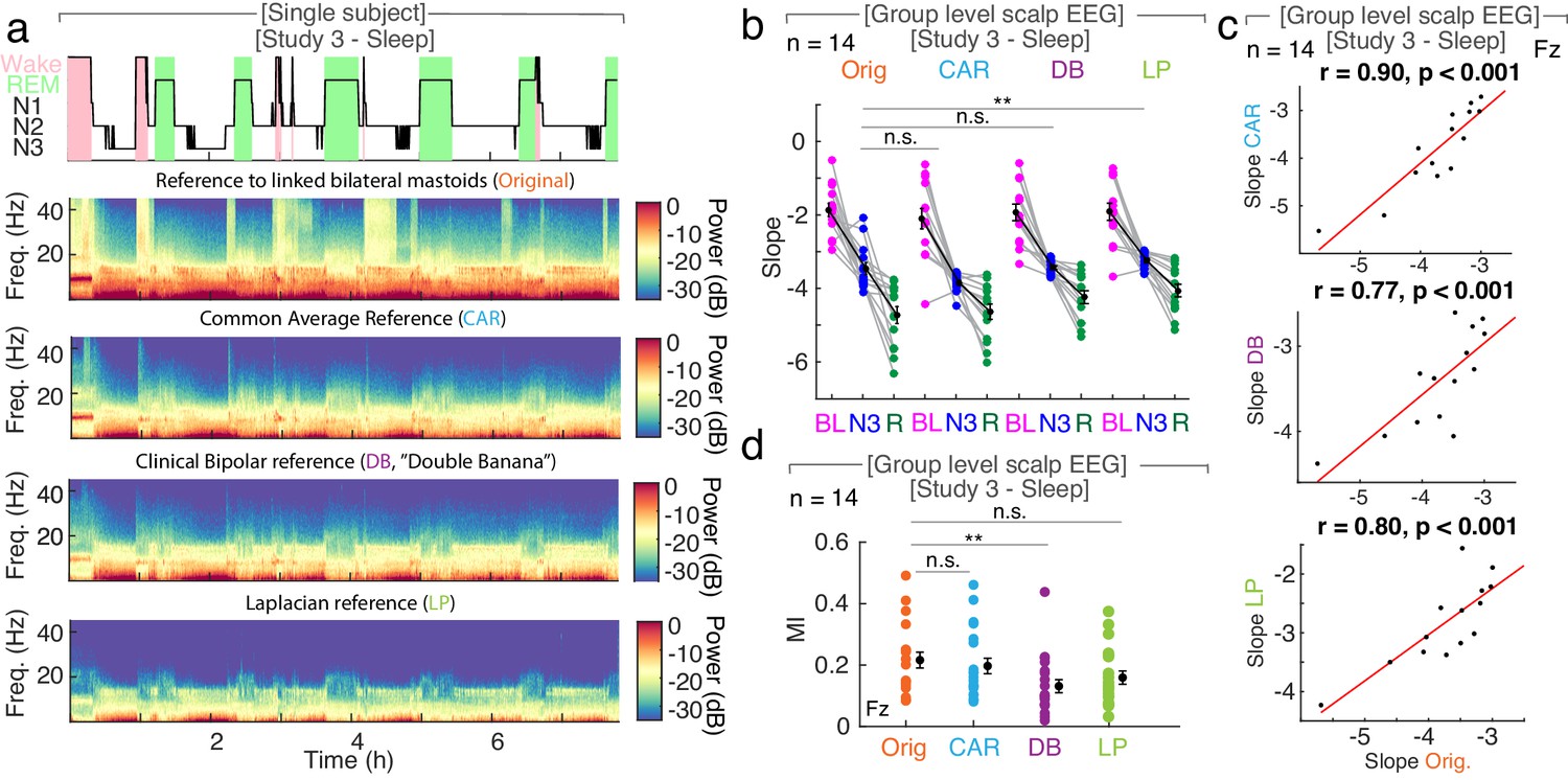
The influence of reference schemes on spectral slope estimation during sleep.
(a) Single subject example of time-resolved average at EEG electrode Fz during a full night of sleep. Upper panel: Expert-scored hypnogram (black), wake (pink), REM (light green). Multitapered time-frequency decomposition using: Upper middle panel – the original reference of linked bilateral mastoids (orange). Middle panel - common average reference (CAR, light blue). Middle lower panel - clinical bipolar reference (‘double banana’ (DB), purple). Lower panel - Laplacian reference (LP, green). (b) 1/f spectral slope in baseline rest (BL, magenta), NREM sleep stage 3 (N3, blue) and REM sleep (REM, green) using the original (Orig., orange), a CAR (light blue), DB (purple) or LP (green) reference in scalp EEG during sleep (n = 14, averaged across electrodes). Paired t-tests (uncorrected): Orig.-CAR: p=0.065, t13 = 2.02, d = 0.36; Orig.-DB: p=0.0875, t13 = −1.85, d = −0.32, Orig.-LP: p=0.005, t13 = −3.35, d = −0.64. n.s. – not significant. **p<0.01. (c) At electrode Fz, 1/f slope values derived from the original (Orig., orange) and the other reference schemes are strongly correlated (n = 14). Upper panel - CAR reference (light blue; r = 0.90, p>0.001), middle panel - DB reference (purple; r = 0.77, p<0.001), lower panel – LP reference (green; r = 0.80, p<0.001). (d) Mutual Information (MI) between hypnogram and 1/f slope derived from power spectra obtained by different reference schemes at electrode Fz (n = 14): Orig. (orange): 0.22 ± 0.04 (black - mean ± SEM), CAR (light blue): 0.22 ± 0.03, DB (purple): 0.15 ± 0.03, LP (green): 0.18 ± 0.03. Paired t-tests (uncorrected): MI Orig.-CAR: p=0.94, t13 = −0.08, d = −0.01; Orig.-DB: p=0.007, t13 = 3.23, d = 0.62, Orig.-LP: p=0.109, t13 = 1.72, d = 0.33. n.s. – not significant. **p<0.01.
Figure 2—figure supplement 9
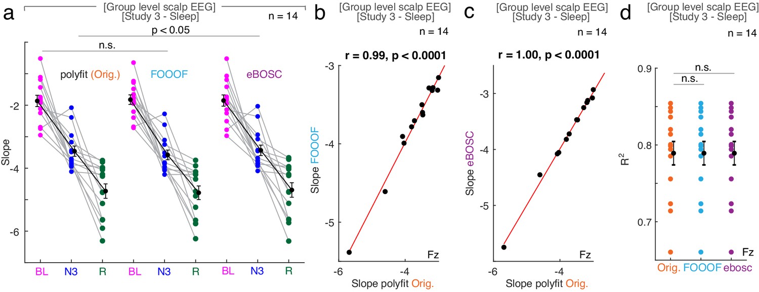
The influence of different fitting algorithms on spectral slope estimation during sleep.
(a) 1/f spectral slope in baseline rest (BL, magenta), NREM sleep stage 3 (N3, blue) and REM sleep (REM, green) using the original polyfit (Orig., orange), the FOOOF (light blue) or eBOSC (purple) algorithm in scalp EEG during sleep (n = 14, averaged across electrodes). Paired t-tests (uncorrected): Orig.-FOOOF: p=0.070, t13 = 1.98, d = 0.11; Orig.- eBOSC: p=0.024, t13 = −2.55, d = −0.06. n.s. – not significant. (b) At electrode Fz, 1/f slope values derived from the original polyfit (Orig., orange) and FOOOF (light blue) are strongly correlated (n = 14; r = 0.99, p<0.0001). (c) At electrode Fz, 1/f slope values derived from the original polyfit (Orig., orange) and eBOSC (purple) are strongly correlated (n = 14; r = 1.00, p<0.0001). (d) Goodness of fit (R2) of the different slope estimates (Orig. - original polyfit (orange); FOOOF (light blue); eBOSC (purple)) to the power spectra in baseline rest, NREM three and REM sleep at electrode Fz (n = 14). Paired t-tests (uncorrected): Orig.-FOOOF p=0.752; Orig.- eBOSC: p=0.117. n.s. – not significant.
Figure 2—figure supplement 10
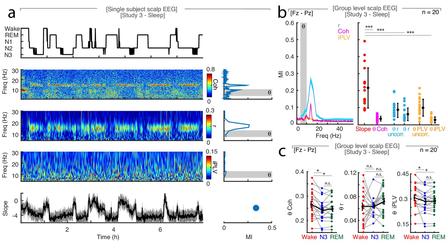
Comparison of Mutual Information captured by fronto-parietal connectivity and spectral slope.
(a) Single subject example: Upper panel – hypnogram. Middle panels – Fz-Pz coherence (Coh), Fz-Pz connectivity measured by orthogonalized power correlation (r) and imaginary phase-locking value (iPLV) between 0.1 and 30 Hz. Right subpanels - Accompanying Mutual Information between the hypnogram and all frequencies; theta (θ; 4–10 Hz) highlighted in gray. Lower panel – spectral slope (30 to 45 Hz) of Fz. Right subpanel – Mutual Information of the Fz slope. (b) Group level (n = 20) analysis of Mutual Information for Fz-Pz coherence and connectivity measured by orthogonalized power correlation (r) or imaginary phase-locking value (iPLV). Left panel – Across all frequencies. Right panel – Comparison of Mutual Information between Fz slope, theta (θ) coherence and connectivity measured by power correlation (uncorrected and orthogonalized) as well as phase-locking value (uncorrected and imaginary). Paired t-test: ***p<0.001. (c) Group level (n = 20) comparison of Fz-Pz theta (θ) coherence, orthogonalized power correlation (r) and weighted phase-locking value (iPLV) between wakefulness, N3 and REM sleep, showing that these metrics do not reliably distinguish between N3and REM sleep. Paired t-test: n.s. – not significant, *p<0.05.
Figure 2—figure supplement 11
Slope difference between N3 and REM sleep.
(a) Scalp EEG (n = 20). Left: Topography of slope difference, Right: Cluster permutation test between slope of N3 and REM. *p<0.05. (b) Depth electrodes (n = 10). Left – Coronal view. Right – Axial view on an MNI brain containing all intracranial electrodes of all patients. Colored – contacts that showed a more negative slope in REM compared to N3 sleep. White – contacts that did not show the pattern.
Figure 3
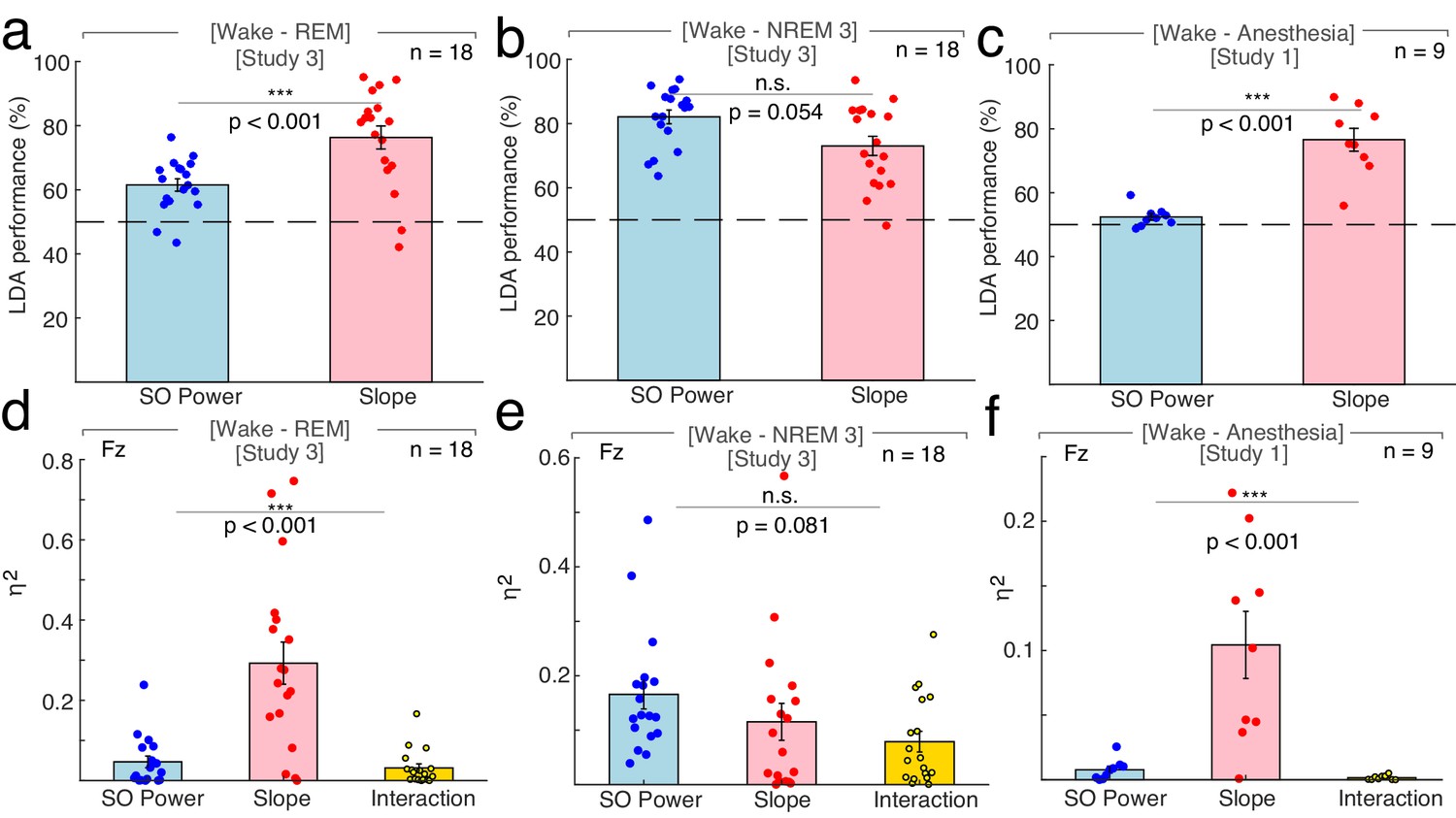
Differentiation of wakefulness from sleep and general anesthesia via Linear Discriminant Analysis (LDA) trained classifier and multivariate general linear modeling (GLM).
All LDA classification performances (panel a – c) were logit-transformed and averaged across channels before comparison. (a) Using the 1/f slope (n = 18; two patients had to be excluded due to insufficient wake trials) resulted in a higher percentage of correct classification of wakefulness and REM compared to slow wave (SO) power (<1.25 Hz; SO: 61.50 ± 1.93% (mean ± SEM), slope: 76.31 ± 3.61%; permutation t-test: p<0.001, observed (obs.) t17 = 3.73, d = 1.25). **p<0.01. Dashed line – chance level at 50% (permutation t-test vs. chance): SO: p<0.001, obs. t17 = 5.51, d = 1.84, slope: p<0.001, obs. t17 = 6.03, d = 2.01). (b) The use of SO power and spectral slope resulted in comparable classification of wakefulness and NREM sleep stage 3 (n = 18; SO: 82.09 ± 2.13%, slope: 73.05 ± 2.97%; permutation t-test: p=0.054, obs. t17 = −1.95, d = −0.72). n.s. – not significant. Dashed line – chance level at 50% (permutation t-tests vs. chance): SO: p<0.001, obs. t17 = 11.23, d = 3.71, slope: p<0.001, obs. t17 = 6.63, d = 2.21). (c) The 1/f slope (n = 9) resulted in a higher classification accuracy of wakefulness and anesthesia with propofol compared to SO power (SO: 52.43 ± 1.04%, slope: 76.56 ± 3.56%; permutation t-test: p<0.001, obs. t8 = 6.10, d = 2.63). ***p<0.001. Dashed line – chance level at 50% (permutation t-test vs. chance): SO: p=0.003, obs. t8 = 2.33, d = 1.10, slope: p<0.001, obs. t8 = 6.15, d = 2.89). All predictors for the multivariate GLM (panel d - f) were z-scored before modeling and calculated on data derived from scalp electrode Fz. (d) Between wakefulness and REM sleep (n = 18; two patients had to be excluded due to insufficient wake trials), the unique explained variance as quantified by eta squared (η2) was significantly different between the 1/f slope, SO power and the interaction between the two (slope: 0.12 ± 0.03, SO: 0.17 ± 0.03, interaction: 0.08 ± 0.02; repeated-measures ANOVA permutation test: p<0.001, F1.16, 19.74 = 19.69). ***p<0.001. (e) Variance between wakefulness and NREM sleep stage 3 (n = 18) was equally well explained by the 1/f slope, SO power and their interaction (slope: 0.12 ± 0.03, SO: 0.17 ± 0.03, interaction: 0.08 ± 0.02; repeated-measures ANOVA permutation test: p=0.081, F1.72, 29.28 = 2.55). n.s. – not significant. f, Out of the total variation between wakefulness and general anesthesia with propofol (n = 9), significantly different proportions could be attributed to the 1/f slope, SO power and their interaction (slope: 0.10 ± 0.03, SO: 0.01 ± 0.003; interaction: 0.002 ± 0.001; repeated-measures ANOVA permutation test: p<0.001, F1.01, 8.09 = 14.61). This effect was mainly driven by the 1/f slope. ***p<0.001.
Figure 4
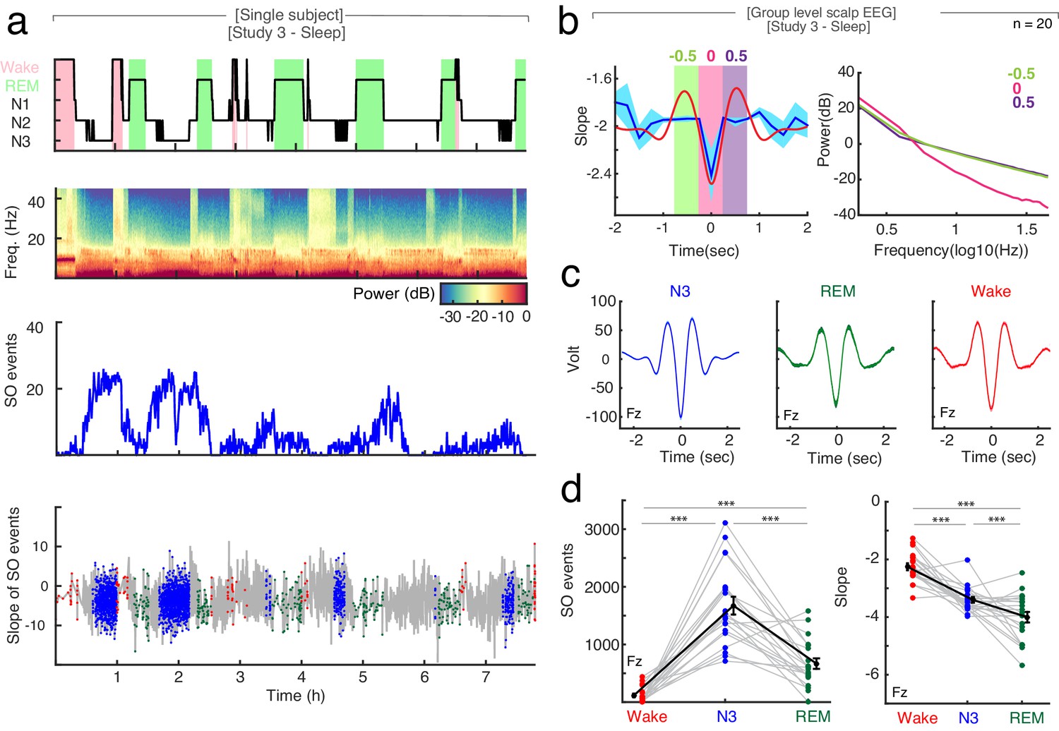
The relationship between spectral slope and slow waves in sleep.
(a) Single subject example: Upper panel: Hypnogram. Wake periods are highlighted in pink, REM periods in light green. Upper middle panel: Multitapered spectrogram of electrode Fz. Lower middle panel: Number of slow wave (SO) events during 30 s segments of sleep in electrode Fz. Note the decreasing number of SO events during the course of the night. Lower panel: Spectral slope of SO events occurring in N3 (blue), wakefulness (red) and REM sleep (green) in electrode Fz. Background: Time-resolved slope of electrode Fz in light gray. (b) Right panel: Average spectral slope changes over the time course of all slow waves in scalp EEG (n = 20) during sleep (blue; mean ± SEM); superimposed in red is the average slow wave of all subjects. Highlighted are the following 0.5 s time windows relative to the slow wave trough: −750 to −250 (center −0.5 s; green), −250 to 250 (center 0 s; pink) and 250 to 750 ms (center 0.5 s; purple). Left panel: Power spectra in log-log space within specified time windows during the slow wave: −750 to −250 (center: −0.5 s; green), −250 to 250 (center: 0 s; pink) and 250 to 750 ms (center: 0.5 s; purple). Note the steep power decrease during the trough of the slow wave (pink). (c) Group level (n = 20) average waveforms in electrode Fz during N3 (blue), REM sleep (green) and wakefulness (red; mean ± SEM). (d) Left: Slow wave events per minute in wakefulness (red), N3 (blue) and REM (green) in scalp EEG channel FZ (n = 20). In black mean ± SEM. Permutation t-tests: ***p<0.001. Right: Slope of slow wave events on the group level (n = 20; averaged across all 19 EEG electrodes) in wakefulness (red), N3 (blue) and REM sleep (green). Mean ± SEM in black. Permutation t-tests: ***p<0.001.
Author response image 1
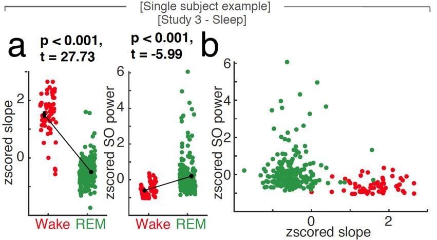
Uni- and multivariate discrimination of wakefulness and REM sleep using the spectral slope and slow oscillation power.
Single subject example at scalp EEG electrode Fz. a, While both 1/f slope (z-scored; left panel) and slow oscillation power (SO, < 1.25 Hz; z-scored; right panel) are able to differentiate wakefulness (red) from REM sleep (green; black: mean ± SEM) in a univariate comparison, the 1/f slope provides most of the discriminative power in a multivariate space as seen in panel b (SO power vs. 1/f slope; both z-scored). Note that the states (red – wakefulness; green – REM sleep) are clearly discernible based on the first feature plotted on the x-axis (the spectral slope) while taking SO power (on the y-axis) into account, does not contribute independent information.
Author response image 2
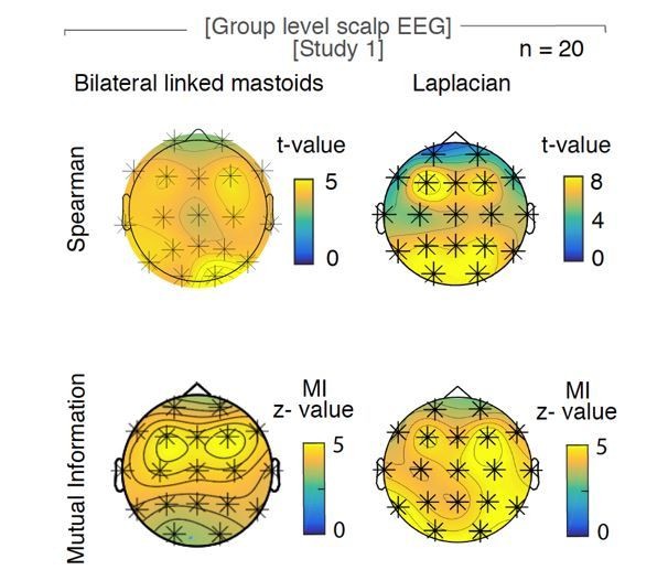
The influence of the choice of reference on the relationship of hypnogram and spectral slope.
Original observation with bilateral linked mastoids reference (left panels) versus Laplacian re-reference (right panels) in scalp EEG recordings during sleep (n = 20). Upper row of topoplots: Cluster permutation test of Spearman rank correlation between hypnogram and time-resolved slope: * p < 0.05. Lower rows of topoplot: Mutual Information between time-resolved slope and hypnogram. Statistics with random block swapping: * p < 0.05.
Author response image 3
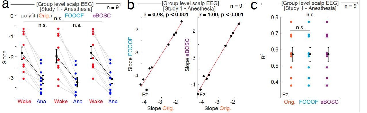
The influence of different fit algorithms on spectral slope estimation in general anesthesia with propofol.
a, 1/f spectral slope in wakefulness (Wake, red) and under anesthesia (Ana, blue) using the original polyfit (Orig., orange), FOOOF (lblue) or eBOSC (purple) algorithm (n = 9, averaged across electrodes). Paired t-tests (uncorrected): Orig.-FOOOF: p = 0.082, t8 = 1.99, d = 0.18; Orig.- eBOSC: p = 0.369, t8 = -0.95, d = -0.03, FOOOF - eBOSC: p = 0.118, t8 = -1.75, d = -0.21. n.s. – not significant. b, At Fz ,1/f slope from original polyfit (Orig., orange) and FOOOF (blue; left panel: r = 0.98, p < 0.001) and original and eBOSC (purple; right panel: r = 1.00, p < 0.001) are strongly correlated.c, Goodness of fit (R2) of the different slope estimates (Orig. - original polyfit (orange); FOOOF (light blue); eBOSC (purple)) to the power spectra in wakefulness and under propofol anesthesia at electrode Fz (n = 9). Permutation t-tests: Orig. - fooof: p = 0.538, Orig. - eBOSC: p = 0.726, fooof - eBOSC: p = 0.690. n.s. – not significant.
Tables
Table 1
Anatomical distribution of stereotactically placed intracranial depth electrodes in Study 2 – Intracranial anesthesia (n = 12).
| Brain region | Total number of electrodes | Electrodes with state-dependent slope modulation |
|---|---|---|
| ALL | 485 | 470 (96.9 %) |
| Prefrontal Cortex (PFC) | 179 | 175 (97.8 %) |
| medial Prefrontal Cortex (mPFC) | 27 | 27 (100 %) |
| lateral Prefrontal Cortex (lPFC) | 147 | 143 (97.3 %) |
| Orbito-frontal Cortex (OFC) | 5 | 5 (100 %) |
| Medial temporal Lobe (MTL) | 40 | 1 (95.0 %) |
| Hippocampus | 26 | 24 (92.3 %) |
| Amygdala | 13 | 13 (100 %) |
| Cingulate Cortex | 22 | 22 (100 %) |
| Insula | 13 | 13 (100 %) |
| M1/Premotor | 48 | 47 (97.9 %) |
| Lateral Temporal Cortex (LTC) | 50 | 50 (100 %) |
| Parietal Cortex | 84 | 78 (92.9 %) |
| Visual Cortex | 49 | 47 (95.9 %) |
Table 2
Anatomical distribution of stereotactically placed intracranial depth electrodes in Study 4 – Intracranial sleep (n = 10).
| Brain region | Total number of electrodes | Electrodes with state-dependent slope modulation |
|---|---|---|
| ALL | 352 | 155 (44.0 %) |
| Prefrontal Cortex (PFC) | 132 | 49 (37.1 %) |
| medial Prefrontal Cortex (mPFC) | 28 | 24 (85.7 %) |
| lateral Prefrontal Cortex (lPFC) | 73 | 15 (20.6 %) |
| Orbito-frontal Cortex (OFC) | 30 | 10 (33.3 %) |
| Medial Temporal Lobe (MTL) | 48 | 33 (68.8 %) |
| Hippocampus | 27 | 19 (70.4 %) |
| Amygdala | 18 | 14 (77.8 %) |
| Cingulate Cortex | 40 | 31 (77.5 %) |
| Insula | 41 | 21 (51.2 %) |
| M1/Premotor | 7 | 7 (100 %) |
| Lateral Temporal Cortex (LTC) | 79 | 13 (16.5 %) |
| Parietal Cortex | 0 | 0 |
| Visual Cortex | 3 | 1 (33.3 %) |
| Other | 2 | 0 |
Key resources table
| Reagent type (species) or resource | Designation | Source or reference | Identifiers | Additional information |
|---|---|---|---|---|
| Software, algorithm | MATLAB Release 2015a and 2018a; Signal Processing Toolbox, Curve Fitting Toolbox, Statistics and Machine Learning Toolbox | The MathWorks Inc, 2020, Natick, Massachusetts, USA | ID_source:SCR_001622 | |
| Software, algorithm | Adobe Illustrator CS6 and CC 2018 | Adobe Inc, 2020, Dublin, Republic of Ireland | ID_source:SCR_010279 | |
| Software, algorithm | FieldTrip 20170829 | Oostenveld et al., 2011; Stolk et al., 2018 | ID_source:SCR_004849 | http://www.fieldtriptoolbox.org/ |
| Software, algorithm | EEGLAB_14_0_0b | Delorme and Makeig, 2004 | ID_source:SCR_007292 | https://sccn.ucsd.edu/eeglab/index.php |
| Software, algorithm | FreeSurfer 5.3.0 | Dale et al., 1999; Fischl, 2012 | ID_source:SCR_001847 | https://surfer.nmr.mgh.harvard.edu/ |
| Software, algorithm | LCMV Beamformer | Van Veen et al., 1997 | ||
| Software, algorithm | IRASA (Irregular Resampling Auto-Spectral Analysis) | Wen and Liu, 2016b | ||
| Software, algorithm | Multitaper Spectral Analysis | Prerau et al., 2017 | ||
| Software, algorithm | FOOOF (Fitting Oscillations and One Over F) | Haller et al., 2018 | https://pypi.org/project/fooof/ | |
| Software, algorithm | eBOSC (extended Better OSCillation detection) | Kosciessa et al., 2020b | https://github.com/jkosciessa/eBOSC | |
| Software, algorithm | Mutual Information | Quian Quiroga and Panzeri, 2009 | http://prerau.bwh.harvard.edu/multitaper/ | |
| Software, algorithm | BioSig Toolbox - Logit transformation | Schlogl and Brunner, 2008 | ID_source:SCR_008428 | |
| Software, algorithm | General Linear Model | Siegel et al., 2015 | ||
| Software, algorithm | Slow wave detection | Helfrich et al., 2018; Staresina et al., 2015 | ||
| Software, algorithm | Random Block Swapping (statistics) | Canolty et al., 2006; Aru et al., 2015 | ||
| Software, algorithm | Connectivity | iPLV (imaginary Phase Lock Value) - Nolte et al., 2004; rhoortho (orhtogonalized power correlation) - Hipp et al., 2012 | ||
| Other | NA |
Author response table 1
| Scalp EEG | original | new |
|---|---|---|
| Anesthesia (n = 9) | 10 second segments | 30 second segments |
| Wakefulness | -1.84 ± 0.30 | -1.85 ± 0.33 |
| Anesthesia | -3.10 ± 0.20 | -2.94 ± 0.18 |
| Sleep (n = 20) | 30 second segments | 10 second segments |
| Baseline rest | -1.87 ± 0.18 | -1.90± 0.19 |
| NREM 3 | -3.46 ± 0.16 | -3.42 ± 0.16 |
| REM | -4.73 ± 0.23 | -4.72 ± 0.22 |
Additional files
Download links
A two-part list of links to download the article, or parts of the article, in various formats.
Downloads (link to download the article as PDF)
Open citations (links to open the citations from this article in various online reference manager services)
Cite this article (links to download the citations from this article in formats compatible with various reference manager tools)
An electrophysiological marker of arousal level in humans
eLife 9:e55092.
https://doi.org/10.7554/eLife.55092


